
CHAPTER 3
Fixed Income – Tactical Asset Allocation
OVERVIEW
This chapter lays out a framework for timing the two primary traditional risk premia in fixed income markets: the term premium and the credit premium. Building on our understanding of the sources of these risk premia discussed in Chapter 2, we will start to think about forecasting when those risk premia are expected to out (under) perform. The framework is designed to be general to identify the relevant inputs for timing models. We are not designing the “best” possible timing models. That arduous task is for the fixed‐income investor. That said, the simple timing models introduced in this chapter show some promise for out‐of‐sample forecasts of risk premia. Data mining concerns are especially important with timing models, as there is a very limited dataset to work with (one history for one asset), so we will discuss the importance of point‐in‐time timing models and unconscious bias that creeps into reworked timing models.
3.1 MARKET TIMING – TERM PREMIUM
3.1.1 Framework for Timing
In Chapter 2 we saw that long‐term US government bonds generated an attractive risk‐adjusted excess (of cash) return over the past century. This is known as the term premium. Obviously, although the term premium has a positive average excess return, there was considerable temporal variation. Indeed, the annualized average excess return was 1.8 percent and the average annualized volatility was 5.1 percent over the past century. The asset owner then asks: Is it possible to vary my exposure to the term premium through time to try and capture more than just the average 1.8 percent return? That is the purpose of this section.
A simple way to think of fixed income return potential is to start with our pricing equations introduced in Chapter 1, which I reproduce here with a discount‐rate term structure (i.e., discount rates vary based on the maturity of the cash flow that is to be discounted). I am using the label ![]() for the discount rate to be used for (risk‐free) government bonds (this captures the rates component of bond returns as described in Chapter 2).
for the discount rate to be used for (risk‐free) government bonds (this captures the rates component of bond returns as described in Chapter 2).

In the case of a government bond, the numerator values are fixed. So, let's rewrite that with fixed coupon, ![]() , and par payments,
, and par payments, ![]() , with no possibility of early or no repayment:
, with no possibility of early or no repayment:

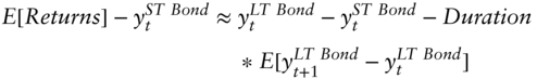
Returns for a government bond are then simply given by the cum‐coupon change in price over the period. We can think of the return potential as driven by changes in prices through time. Looking at Equation (3.2), the uncertainty stems from the expectations operator in the denominator. How yields are expected to change over time will determine government bond returns. We can write an approximation for returns as follows:

To be clear, this is an approximation simply to illustrate that changing expectations about the discount rate will determine the change in government bond prices and hence the return. The other component of the return is governed by the initial yield: ownership of the bond carries participation rights in the expected, and in this case known, coupons and principal payments. As discussed in Chapter 1, at the time of purchase of the bond the price of the bond implies a yield to maturity. So our expected return has two broad components:
We now have our simple framework. Our timing model for the term premium will focus on these two components of expected excess returns (i.e., in excess of cash to be consistent with our definition of term premium at the start of the chapter). First, we have the initial yield. More generally, this can be thought of as the “carry” associated with the government bond position. Second, we have the expected change in yields over the investor's holding period. Technically, this change in yield needs to be multiplied by duration to convert the expected change in yield to an expected return.

EXHIBIT 3.1 Visual representation of the expected return for a risk‐free bond from “carry.”
Exhibit 3.1 provides a simple representation of what “carry” is. If nothing happens but the passage of time, carry is the return you will receive. In the case of our risk‐free government bond from Equation (3.4), this means that the return we get from carry is the price change for our bond when the discount‐rate term structure remains unchanged, but, we are now discounting the fixed set of coupon and principal payments after rolling the cash flows forward (i.e., we are repricing the bond cash flows with the same discount rates, but because the cash flows are shifted forward they are discounted at different rates). We can write the approximate expected excess return (here the excess of cash is explicit) assuming the discount rate structure remains unchanged as:

Equation (3.6) is approximate, because we have made use of duration and are working with a linear, first‐order approximation of expected returns. We are ignoring higher‐order moments of yield curve changes. This simply says that a measure of carry should reflect the current yield to maturity and expected changes in yields from the passage of time (i.e., yield curve does not change its shape).
For our measure of carry we will use what is called the term spread, ![]() , the difference in the nominal long‐term government bond yield and the nominal short‐term government yield (labeled by the thick black arrow in Exhibit 3.1). This is simply the first portion of Equation (3.6). We are making this choice for data expediency. As we will discuss in Section 3.1.b, our data access for the last century does not include rich data of the entire yield curve, so this approximation is out of necessity. As depicted in Exhibit 3.1, this simple measure will miss curvature in the yield curve and the associated “roll‐down” component (labeled by the thin black arrow in Exhibit 3.1). This “roll‐down” captures the expected change in yield from the passage of time. This gives a better measure of “carry,” but still leaves open the possibility of other expected changes in yields (and hence returns).
, the difference in the nominal long‐term government bond yield and the nominal short‐term government yield (labeled by the thick black arrow in Exhibit 3.1). This is simply the first portion of Equation (3.6). We are making this choice for data expediency. As we will discuss in Section 3.1.b, our data access for the last century does not include rich data of the entire yield curve, so this approximation is out of necessity. As depicted in Exhibit 3.1, this simple measure will miss curvature in the yield curve and the associated “roll‐down” component (labeled by the thin black arrow in Exhibit 3.1). This “roll‐down” captures the expected change in yield from the passage of time. This gives a better measure of “carry,” but still leaves open the possibility of other expected changes in yields (and hence returns).
The second component of expected excess returns in Equation (3.4) is the expected change in yields. For this, we will lean heavily on recent research (e.g., Asness, Moskowitz, and Pedersen 2013, and Asness, Ilmanen, and Maloney 2017) and group our timing models into two broad categories: value and momentum. Both measures are designed to forecast changes in yields. In the case of momentum, that is for continuation in recent yield changes. In the case of value, that is for expected reversal of current yields to a “normal” level of yields.
How should we think about measuring momentum and value for a government bond timing model? We will use the same approach as in Asness, Ilmanen, and Maloney (2017) and extend the time series to the end of 2020. The measure of momentum will be the 12‐month arithmetic average of government bond excess (of cash) returns. The measure of value will be real bond yields computed as the nominal yield on long‐term government bonds less a survey‐based forecast of long‐term inflation.
3.1.2 Data (Some Details)
Our term premium timing model will be assessed on data sourced from Global Financial Data. This data vendor is selected because they maintain very long time series of market data across many asset classes and geographies. We limit our analysis of timing term premium to the period 1920–2020 primarily due to Treasury Bill data. Although Treasury bills (one‐month) were only formally introduced in 1929, Global Financial Data can source Treasury instruments with a slightly longer maturity (three to six months) to complete the series back to 1920. Treasury bill secondary market prices and yields are computed as the averages of the bid rates quoted by a sample of primary dealers who report to the Federal Reserve Bank of New York. We use prices and yields as of the close of the last trading day each month to compute (i) T‐bill yield (used as a component of our carry measure), and (ii) T‐bill returns (used as our measure of cash returns).
Data for the yields and returns of long‐term government bonds are also from Global Financial Data. Over our 1920–2020 period, long‐term government bond yield and return data are linked to the Federal Reserve Board's 10–15 Treasury Bond Index for the 1920–1941 period, and specific 10‐year bonds are used from 1941 onward. This data is used to compute (i) US government bond nominal yield (used as part of the real bond yield value measure), and (ii) US government bond total returns (used to compute US government bond excess returns, our primary variable of interest to forecast).
Data for long‐term inflation expectations comes from multiple sources (thank you to Antti Ilmanen for graciously sharing this data). From 1920 to 1955, statistical estimates based on a weighted average of past 10‐year inflation rates are used. From 1955–1978 statistical estimates of long‐term inflation expectations from Kozicki‐Tinsley (2006) are used (their statistical estimates use a different weighting function that also makes use of near‐term survey forecasts of inflation). From 1978–1989 an average across multiple surveys is used (e.g., Survey of Professional Investors, Livingston, Blue Chip Economic Indicators, and Consensus Economics). Finally, for the 1990–2020 period, the average annual inflation forecasted for the next decade (Consensus Economics) is used. This data series is used directly in the construction of real bond yield, the value measure.
3.1.3 Converting Raw Data to Signals
We can now assess whether, and how, our return forecasting framework works. To do this we need to create a time series of “signals” that indicate our willingness to increase or decrease our exposure to long‐term government bonds (term premium). We will assess our skill from the perspective of a real money investor who needs to remain invested in the fixed income markets, but is able to dial up or down the amount of capital invested into the market at any specific point in time.
We have three investment signals: (i) value (measured as real bond yield, the difference between nominal long‐term government bond yields and long‐term inflation forecasts), (ii) momentum (measured as the most recent 12‐month arithmetic average of long‐term government bond excess returns, and (iii) carry (measured as the term spread, or difference between long‐term government bond nominal yields and short‐term government bill nominal yields).
For each of these three measures we need to convert them to a “signal.” It is important that we do not make use of any future information when constructing these signals (that would be cheating). For each measure we will conduct the following transformations: (i) extreme value treatment (to help reduce the influence of extreme values we will cap and floor each signal based on the expanding 95th and 5th percentile values, respectively), (ii) benchmarking (we will subtract from the current realization of the unprocessed signal the expanding median value of its value), (iii) volatility scaling (we will divide that benchmark adjusted value by a measure of volatility, we will use a nonparametric method computed as an expanding window of the difference between the 95th and 5th percentile value of the respective signal), and (iv) timing curves (our effectively Z‐scored signal is converted to a value that can be applied to the capital invested in long‐term government bonds, we will use a simple linear capped and floored transformation that is restricted to be between 50 and 150 percent invested in bonds). These choices mirror those made in Asness, Ilmanen, and Maloney (2017).
3.1.4 Scatter Plots
It is easiest to see how these various transformations affect the raw values of signals visually. Exhibit 3.2 consists of four panels that illustrate the impact of each transformation on our real bond yield value signal. Panel A is a scatter plot reflecting the impact of treatment of extreme values. At first glance this may look surprising, as there is not a concentration of data points at a global extreme value. This is because the capping and flooring is done each month using all data available up until that point. Consequently, what is extreme is an evolving concept over time. The correlation between the original and capped/floored values is 0.96.
Panel B is a scatter plot reflecting the impact of benchmarking and volatility scaling. This transformation is changing the information contained in real bond yields over the full period. What is going on? This is because our analysis needs to be at a point in time. For each month we can only make use of the information that was available at that point in time. Thus, the benchmarking is based on a median of real bond yield using all data up to the month of interest, and the nonparametric volatility scaling is also only using information on the distribution of real bond yields up to the month of interest. The correlation between the capped/floored real bond yield and the fully transformed value signal is 0.86. In contrast, if we had used a full‐sample median and full sample 95th less 5th percentile deflator we would have a correlation of 1. This is not a loss of information from a tactical asset allocation perspective. You can only use information that is available to you at the relevant time.
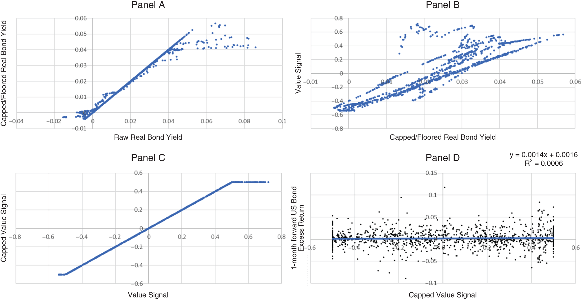
EXHIBIT 3.2 Value signals – term premium. Panel A shows the effect of capping and flooring values at the 95th and 5th percentile (expanding window). Panel B shows the effect of benchmarking and volatility scaling (nonparametric Z‐scoring of the capped signal). Panel C shows the final signal timing curve. Panel D shows the link between value timing and one‐month‐ahead long‐term government bond excess returns.
Sources: Described in text, period 1920–2020.
Panel C then shows the impact of our selected timing curve. This has the expected shape as all values more than 0.5 in absolute value are floored and capped at −0.5 and +0.5, respectively. This monotone transformation is one way to scale the strength of your convictions in the signal. There is a lot of choice here. Our choice is linear in the transformed real bond yield signal between −0.5 and +0.5. We are choosing not to tactically vary our positions in government bonds too much. Alternative choices could be placing even less weight on central values and only taking active positions when your signal is sufficiently large in either direction.
Finally, we are now able to assess whether our simple value measure has any out‐of‐sample success in timing exposure to the term premium. Panel D shows the data. The vertical axis is the one‐month forward excess return of long‐term government bonds, and the horizontal axis is the fully transformed value signal. The line of best fit is shown on the exhibit and it has an ![]() of 0.0006, which corresponds to a correlation (information coefficient) of 0.024. This is a small correlation coefficient and suggests value signals, at least as we have chosen to measure them, have only limited success in timing exposure to the term premium.
of 0.0006, which corresponds to a correlation (information coefficient) of 0.024. This is a small correlation coefficient and suggests value signals, at least as we have chosen to measure them, have only limited success in timing exposure to the term premium.
Exhibit 3.3 and Exhibit 3.4 show scatter plots for momentum and carry, respectively. Capping and flooring extreme values has minimal impact on the information content of each signal (Panel A). There is a similar less‐than‐perfect correlation between the capped signals and the benchmarked and volatility scaled transformed signal (Panel B) with a correlation of 0.90 and 0.95 for momentum and carry, respectively. Again, this is attributable to the point‐in‐time nature of our forecasting exercise. Both momentum and carry have the same timing curve applied (Panel C). Finally, the investment efficacy of momentum and carry are superior to value (Panel D). Specifically, the correlation of the fully transformed momentum (carry) signal and one‐month forward excess return of long‐term government bonds is 0.061 (0.107), respectively.
A natural question to then ask is, how do these investment signals work individually and in combination? Our investment decision was to decide whether to invest $1 into long‐term government bonds each month or some other allocation of between $0.50 and $1.50, based on the respective investment signal. The active return is then the excess of cash return of the outperformance attributable to that investment signal. Exhibit 3.5 provides a summary of the active investment return potential for the various signal combinations.
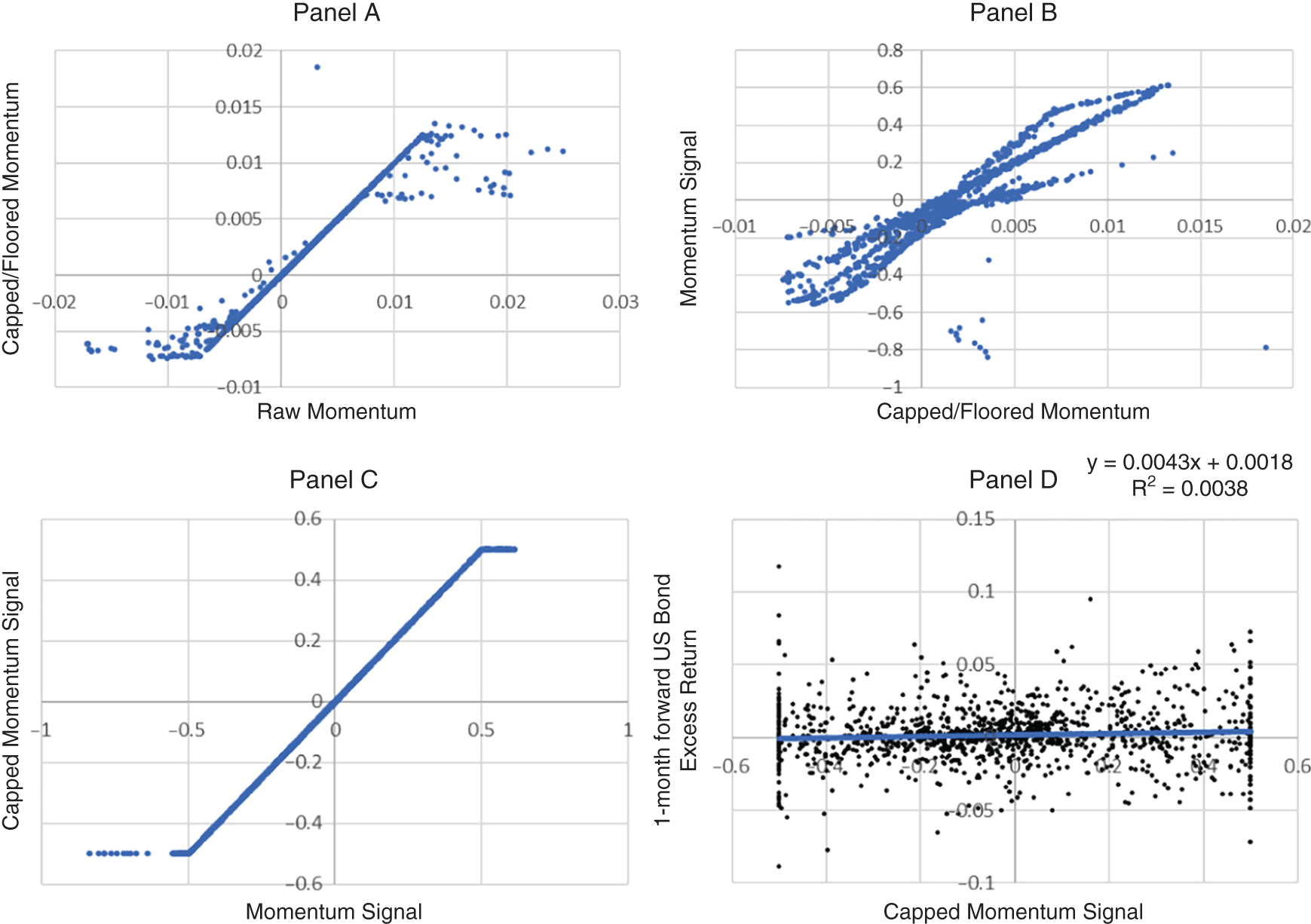
EXHIBIT 3.3 Momentum signals – term premium. Panel A shows the effect of capping and flooring values at the 95th and 5th percentile (expanding window). Panel B shows the effect of benchmarking and volatility scaling (nonparametric Z‐scoring of the capped signal). Panel C shows the final signal timing curve. Panel D shows the link between momentum timing and one‐month‐ahead long‐term government bond excess returns.
Sources: Described in text, period 1920–2020.
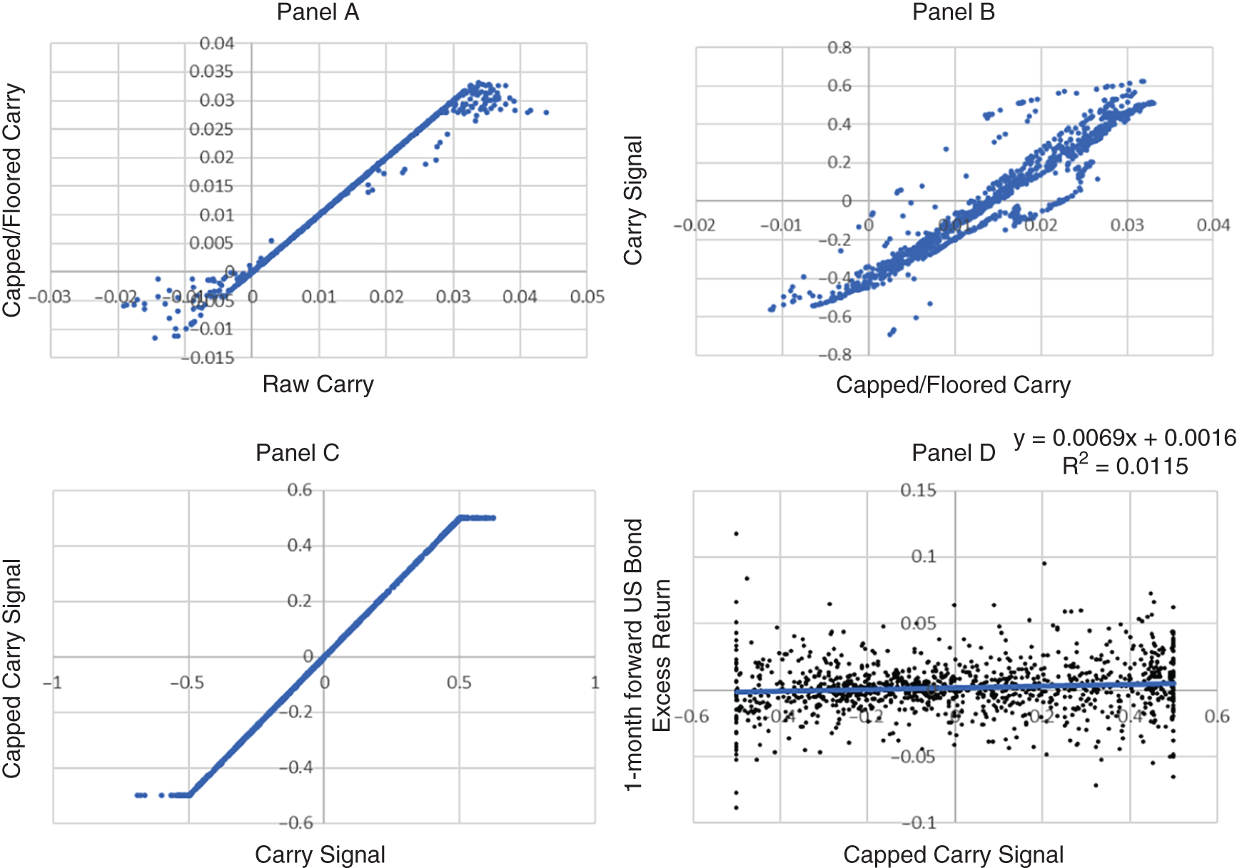
EXHIBIT 3.4 Carry signals – term premium. Panel A shows the effect of capping and flooring values at the 95th and 5th percentile (expanding window). Panel B shows the effect of benchmarking and volatility scaling (non‐parametric Z‐scoring of the capped signal). Panel C shows the final signal timing curve. Panel D shows the link between carry timing and one‐month‐ahead long‐term government bond excess returns.
Sources: Described in text, period 1920–2020.
EXHIBIT 3.5 Active returns from tactically timing term premium.
| Value | Momentum | Carry | Value + Momentum | Value + Momentum + Carry | |
|---|---|---|---|---|---|
| Average | 0.16% | 0.35% | 0.76% | 0.27% | 0.42% |
| Std. Dev. | 0.0222 | 0.0228 | 0.0242 | 0.0150 | 0.0148 |
| Sharpe | 0.07 | 0.15 | 0.31 | 0.18 | 0.29 |
| Alpha (ann.) | −0.02% | 0.37% | 0.68% | 0.18% | 0.35% |
Sources: Described in text, period 1920–2020.
The correlation across the active return series is informative to help understand the return profile of the combinations of signals. Value and momentum have a modest negative correlation of −0.17, value and carry have a very low correlation of 0.01, and momentum and carry have a positive correlation of 0.48 (part of this higher correlation is due to the use of total returns as the measure of momentum that includes the realization of carry). The combination of value and momentum, and value and momentum and carry, are formed by simple averages of the underlying fully transformed individual signals. Given their low pairwise correlations, it is not surprising to see improved risk‐adjusted returns from the combinations. This is diversification at work.
Although the Sharpe ratios are all positive, the magnitude is small compared to the full sample Sharpe ratio for the term premium (0.35). The astute reader will notice that this Sharpe ratio is slightly different than the 0.34 quoted in Chapter 2 (this is due to a slightly longer time period and different data source used here). The average excess return for long‐term government bonds is around 2 percent for the 1920–2020 period. Except for carry, the “alphas” in Exhibit 3.5 are small relative to the term premium itself (of course, leverage can be applied to a long/short implementation of the various timing signals to increase the level of returns). Furthermore, these active investment decisions all require active trading, which would incur additional trading costs. The returns that we have looked at are all before accounting for implementation costs. In summary, the small timing returns are the basis for the working title of the paper on which this analysis was based: “Sin a Little” (Asness, Ilmanen, and Maloney 2017).
3.1.5 Skill in Timing
Another way to visualize the investment return potential from tactically timing exposure to the term premium is to track cumulative excess return performance and the associated outperformance for each of the signals individually. This can help place the relative scale of returns into context. Exhibit 3.6 shows the cumulative excess returns to a buy‐and‐hold position in long‐term government bonds (solid black line). This is what a Sharpe ratio of 0.35 looks like (over the long run, your wealth is a lot more than where it started from, $1 in this chart, but there are some ugly periods along the way, the middle decades of the 1900s). The full tactical timing model that made equal use of value, momentum, and carry signals has an even more attractive cumulate excess return profile (solid gray line). This is the net benefit of our investment insights outlined in the prior section. When we strip out the outperformance of each individual signal (dashed lines), the return potential here is small relative to the passive exposure to the term premium. Therefore, people say, “sin a little” (there is some evidence of out‐of‐sample return predictability for timing exposure to the term premium, but the magnitude of that return is small relative to the amount of risk taken).
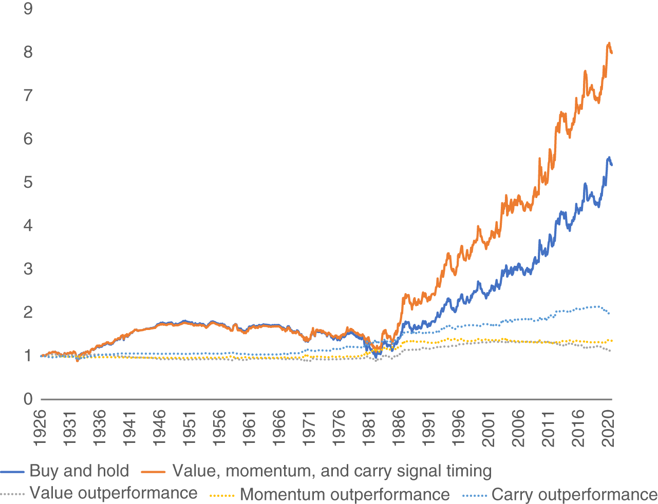
EXHIBIT 3.6 Cumulative excess returns from long‐term government bonds and associated tactical exposures.
Sources: Described in text, period 1920–2020.
3.1.6 Extensions
Everything we have explored for tactical investment decisions is based on sound economic principles. However, the precision and breadth of information we have looked at to measure carry and forecast expected changes in yields was deliberately limited. Our purpose was to lay out a framework. A user is then free to improve the specific investment insights to make better tactical investment decisions. Later, I discuss various avenues that asset owners and investors may wish to consider for their tactical investment decisions for term premium.
Our carry measure only captured the term spread. This makes only limited use of information in the shape of the yield curve. In developed markets like the United States there are many bonds trading in secondary markets (and associated interest rate derivatives). From these secondary market prices, it is possible to build a zero‐coupon bond yield curve. With this granular zero curve, you can then re‐price a given bond on a roll‐forward basis (e.g., 6 or 12 months later). Comparing the two prices of the bond, cum‐coupon, will provide a more comprehensive measure of carry that makes complete use of yield curve information.
Our momentum measure only made use of the most recent 12 months of bond excess returns. Although there is a lot that could be done by altering the look‐back period and weighting schema used for momentum, I think that is an exercise prone to in‐sample data mining. Careful thought should be given to the measure of price momentum. Do you want to use total or excess return momentum? Return momentum includes the realization of carry, which you may not want to include, leaving carry as a separate signal. Additionally, asset owners and investors should give thought to what are the determinants of yields (see Chapter 2) and use those insights to broaden measures of momentum. For example, we saw in Chapter 2 that risk‐free government bond yields are intrinsically linked to economic growth and inflation expectations. Thus, measures of the real economy (industrial production, GDP, aggregate employment, capacity utilization) and inflation expectations can be used directly as additional measures of momentum. Government bonds have a negative sensitivity to both economic growth and inflation, so momentum in growth and inflation would be a negative signal for the term premium. Brooks (2017) provides a useful summary of the types of approaches that could be used to capture non‐price‐based measures of momentum relevant for the fixed income market.
Finally, our value measure was very crude. Chapter 2 made it clear that long‐term inflation expectations are but one of the determinants of yields. If we are trying to build a forecast of where yields are likely to move to, we should explore what macroeconomic models have to offer. There are many such models to choose from, but they generally provide structure (i) linking how current short‐term interest rates will evolve over the life of the long‐term government bond (e.g., a statistical or economically motivated path of future interest rates), and (ii) anchoring longer‐term interest rates (e.g., to economic growth and productivity and long‐term inflation expectations). Armed with information on the structural determinants of yields, you can then estimate the distance between actual yields and model yields. This gap can be thought of as a “term premium” but, depending on construction, may also be your forecast of expected yield changes.
There are clearly a lot of potential extensions of the term premium tactical timing model that we have discussed. One important caveat should be kept in mind though. Despite all the effort that could be expended on improving the tactical investment decision, this is an inherently low‐breadth investment choice (see e.g., Grinold and Kahn 2000). You can either over‐ or underweight your exposure to long‐term government bonds (long‐only investor) or long or short interest rate derivatives (unconstrained long/short investor). For both investor types the low breadth implies that the amount of risk allocated to these tactical decisions should be moderate. Remember the adage “sin a little.”
3.2 MARKET TIMING – CREDIT PREMIUM
3.2.1 Framework for Timing
We will use a similar framework for thinking about tactical investment decisions for corporate bonds, with one key exception. As Chapter 2 demonstrated, the unique source of return potential for corporate bonds is the return over and above risk‐free yields. Our focus now is on credit‐excess returns.
We can extend Equation (3.3) to allow for both risk‐free and risky components of discount rates (![]() reflects the risk‐free portion and
reflects the risk‐free portion and ![]() the risky portion). Using the language from Chapter 2,
the risky portion). Using the language from Chapter 2, ![]() captures the rates component of corporate bond returns, and
captures the rates component of corporate bond returns, and ![]() captures the spread component of corporate bond returns. The return approximation in Equation (3.7) notes that changing expectations of both the risk‐free and risky components of discount rates will generate returns. We will ignore the risk‐free portion here (that was covered in the previous section). In practice, this means that we are looking at interest‐rate hedged portfolios of corporate bonds or credit index derivatives.
captures the spread component of corporate bond returns. The return approximation in Equation (3.7) notes that changing expectations of both the risk‐free and risky components of discount rates will generate returns. We will ignore the risk‐free portion here (that was covered in the previous section). In practice, this means that we are looking at interest‐rate hedged portfolios of corporate bonds or credit index derivatives.

This approximation helps to identify the importance of changes in credit spreads, ![]() , and how they affect corporate bond prices. Credit spreads and, more specifically, the term structure of credit spreads imply an initial expected credit‐excess return. The discussion for carry in the context of government bonds applies here too, except that the curve we are talking about is for credit spreads, not risk‐free yields. So, our expected credit excess return has two broad components:
, and how they affect corporate bond prices. Credit spreads and, more specifically, the term structure of credit spreads imply an initial expected credit‐excess return. The discussion for carry in the context of government bonds applies here too, except that the curve we are talking about is for credit spreads, not risk‐free yields. So, our expected credit excess return has two broad components:
We have our framework. First, there is the “carry” component of credit excess returns. This is the expected return if the shape of the credit‐term structure remains unchanged. Estimating the carry component of corporate bonds can be quite challenging, but the idea is to re‐price a given corporate bond, or a portfolio of corporate bonds, using the same credit curve but rolling forward all associated cash flows.
Second, we have a catchall component of returns for the changes in credit spreads. For this, we will lean on research examining cross‐sectional predictability of credit spreads and credit excess returns (e.g., Houweling and van Zundert 2017 and Israel, Palhares, and Richardson 2018). Value and momentum are common investment themes in these papers, and both are designed to forecast changes in credit spreads. In the case of momentum, that is for continuation in recent changes in credit spreads. In the case of value, that is for expected reversal of credit spreads to a “normal” level.
We will use a simple price‐based measure of momentum: the 12‐month arithmetic average of index level corporate bond excess returns. Our measure of value is based on an expanding window regression as follows:
Spread is the index‐level option‐adjusted spread (this is the credit spread adjusted for the expected exercise of any embedded options in the underlying corporate bonds that would affect the duration profile and hence yield of the corporate bond). Leverage is the average market leverage of US firms (approximated by Russell 1000 index constituents) measured as the market value of equity plus the book value of all net debt (including minority interest and preferred stock) divided by the market value of equity. Profitability is the average profitability of US firms (using gross profits divided by total assets). Volatility is the average total return volatility for US large capitalization firms using BARRA risk model (USE3). The three explanatory variables are measured monthly using trailing 12‐month data. As expected, the regression coefficients on leverage and volatility are strongly positive (for US investment‐grade (IG) corporate bonds ![]() is 1.63 with a test statistic of 23.5,
is 1.63 with a test statistic of 23.5, ![]() is 2.81 with a test statistic if 9.89; for US high yield (HY) corporate bonds
is 2.81 with a test statistic if 9.89; for US high yield (HY) corporate bonds ![]() is 4.43 with a test statistic of 22.4,
is 4.43 with a test statistic of 22.4, ![]() is 11.97 with a test statistic if 14.88) and the regression coefficient for profitability is strongly negative (for US IG corporate bonds
is 11.97 with a test statistic if 14.88) and the regression coefficient for profitability is strongly negative (for US IG corporate bonds ![]() is −8.07 with a test statistic of −11.07; for US HY corporate bonds
is −8.07 with a test statistic of −11.07; for US HY corporate bonds ![]() is −12.91 with a test statistic of −5.49).
is −12.91 with a test statistic of −5.49).
We estimate Equation (3.9) separately for the US IG corporate and US HY corporate markets. We use an expanding window regression starting in 1990 for US IG and 1994 for US HY. Thus, our value measures cover a shorter period than what is available for momentum (starts in 1988 for US IG and 1989 for US HY) and carry (starts in 1989 for US IG and 1994 for US HY).
3.2.2 Data (Some Details)
Our credit‐premium timing model will be assessed on data sourced from Bloomberg Indices. We will examine both IG and HY corporate bond indices. A benefit of the IG index is that it had a longer time series, whereas the benefit of the HY index, as we saw in Chapter 2, is that there is more credit premium and variability in credit excess returns in the HY market. And the magnitude and variability of the credit premium is a necessary condition for tactical investment decisions to be economically meaningful. Our data will be from 1989–2020 for the US IG index and 1994–2020 for the US HY index. Although we can measure momentum (using excess returns) in the HY markets back to 1990, option adjusted spreads (necessary for both carry and value measures) are only available from 1994 onward.
3.2.3 Converting Raw Data to Signals
We can now assess whether, and how, our return forecasting framework works. We need to create a time series of “signals” that indicate the relative attractiveness of corporate bonds (credit premium). Consistent with our analysis of the term premium, we will assess our skill from the perspective of a real money investor who needs to remain invested in the fixed income markets, but is able to dial up or down the amount of capital invested into the market at any specific point in time.
We have three investment signals: (i) value (measured as the regression residual from an expanding window regression of index‐level credit spreads projected onto measures of average profitability, leverage, and volatility for a typical US firm), (ii) momentum (measured as the most recent 12‐month arithmetic average of corporate bond excess returns), and (iii) carry (measured as the credit spread).
For each of these three measures we need to convert them to a “signal.” We use the same transformation procedure as we did for the term premium. Please refer to Section 3.1.3 for a reminder.
3.2.4 Scatter Plots
Let's start with an examination of the three signals individually. Exhibits 3.7, 3.8, and EXHIBIT 3.9 show scatter plots for value, momentum, and carry for the US IG corporate bond market, respectively. Exhibits 3.10, 3.11, and EXHIBIT 3.12 show scatter plots for value, momentum, and carry for the US HY corporate bond market, respectively. The structure of these exhibits is like what was shown previously for analysis of the term premium. Across all signals and both corporate bond markets the impact of capping and flooring extreme values is small (and behaves exactly as expected), and the benchmarked and volatility scaled transformed signal preserves a lot of the information of the raw signals (the correlations between the capped signals and the transformed signal vary between 0.82 and 0.93 for US HY and between 0.82 and 0.84 for US IG). Again, the lack of perfect correlation is attributable to the point‐in‐time nature of our forecasting exercise. All measures use the same timing curve. Finally, the investment efficacy of value, momentum, and carry are shown in the bottom right (Panel D) of each exhibit. Credit‐premium timing in the US IG markets over the 1989–2020 period has been less successful than the US HY markets. Specifically, the correlations of value, momentum, and carry timing with one‐month forward US IG corporate bond index credit excess returns are 0.01, −0.01, and 0.06, respectively. In contrast, the correlations of value, momentum, and carry timing with 1‐month‐forward US HY corporate bond index credit‐excess returns are 0.09, 0.08, and 0.03, respectively.
There are striking differences in the timing‐model performance across IG and HY markets. First, there is lower predictability in IG markets, perhaps due to the lower magnitude and variability of credit‐excess returns (there is just less credit premium to be tactically timed). Second, there are differences in the relative performance of the signals. Momentum works better in HY markets, and carry works better in IG markets. The finding of momentum working less well in safer corporate bonds is evident in the cross‐section of corporate bond returns, so it is not surprising to see that result translate to the index level (e.g., Israel, Palhares, and Richardson 2018).
A natural question to then ask is how do these investment signals work individually and in combination. Exhibits 3.13 (US IG) and 3.14 (US HY) provide a summary of the active returns from the respective timing signals, both individually and in combination. The active return is then the excess of cash return of the outperformance attributable to that investment insight (in excess of the return from the credit market itself).

EXHIBIT 3.7 Value signals – Credit Premium (US IG). Panel A shows the effect of capping and flooring values at the 95th and 5th percentile (expanding window). Panel B shows the effect of benchmarking and volatility scaling (nonparametric Z‐scoring of the capped signal). Panel C shows the final signal‐timing curve. Panel D shows the link between value timing and one‐month‐ahead IG corporate bond index excess returns.
Sources: Described in text, period 1989–2020.
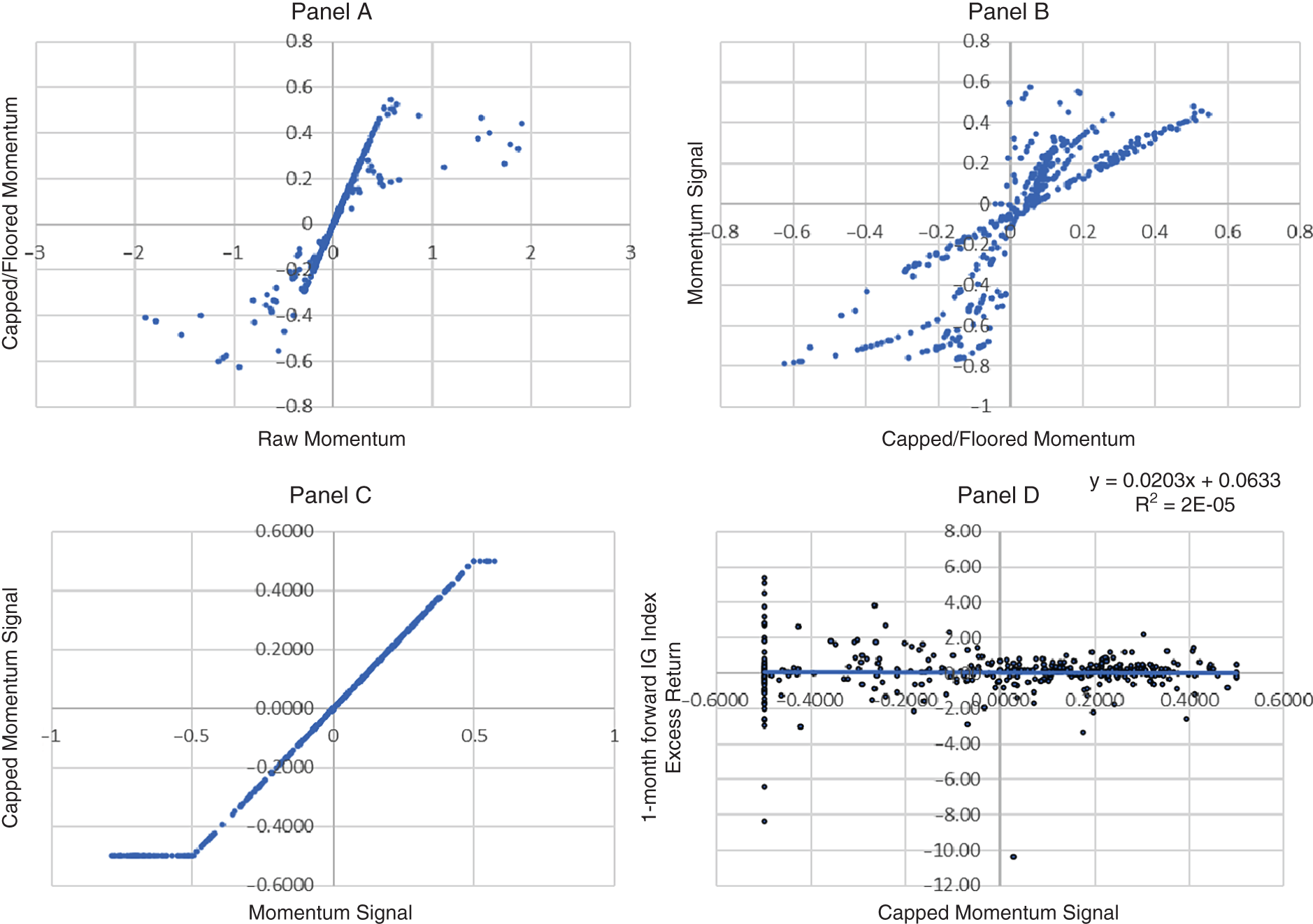
EXHIBIT 3.8 Momentum signals – Credit Premium (US IG). Panel A shows the effect of capping and flooring values at the 95th and 5th percentile (expanding window). Panel B shows the effect of benchmarking and volatility scaling (nonparametric Z‐scoring of the capped signal). Panel C shows the final signal‐timing curve. Panel D shows the link between momentum timing and one‐month‐ahead IG corporate bond index excess returns.
Sources: Described in text, period 1989–2020.
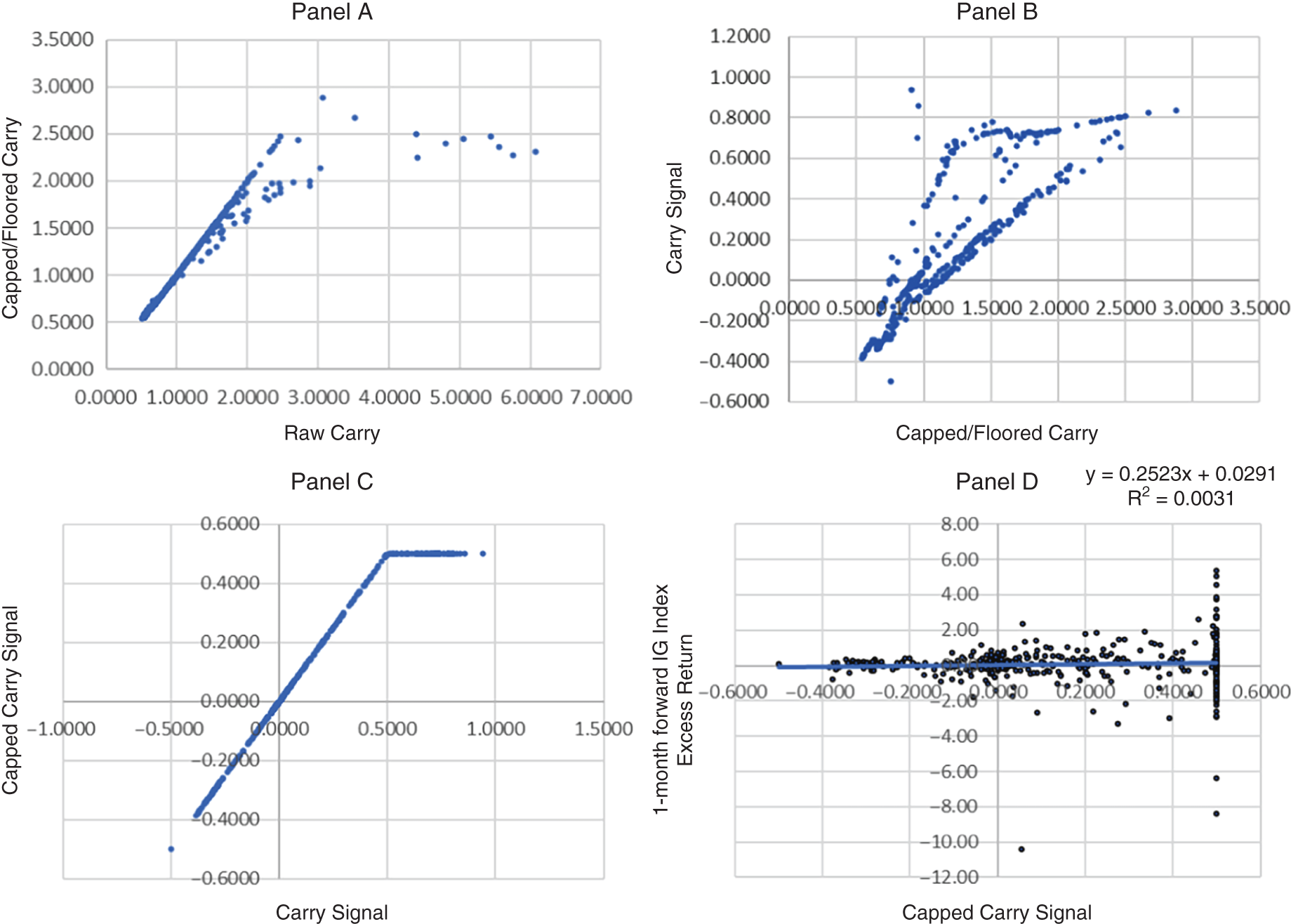
EXHIBIT 3.9 Carry signals – Credit Premium (US IG). Panel A shows the effect of capping and flooring values at the 95th and 5th percentile (expanding window). Panel B shows the effect of benchmarking and volatility scaling (nonparametric Z‐scoring of the capped signal). Panel C shows the final signal‐timing curve. Panel D shows the link between carry timing and one‐month‐ahead IG corporate bond index excess returns.
Sources: Described in text, period 1989–2020.
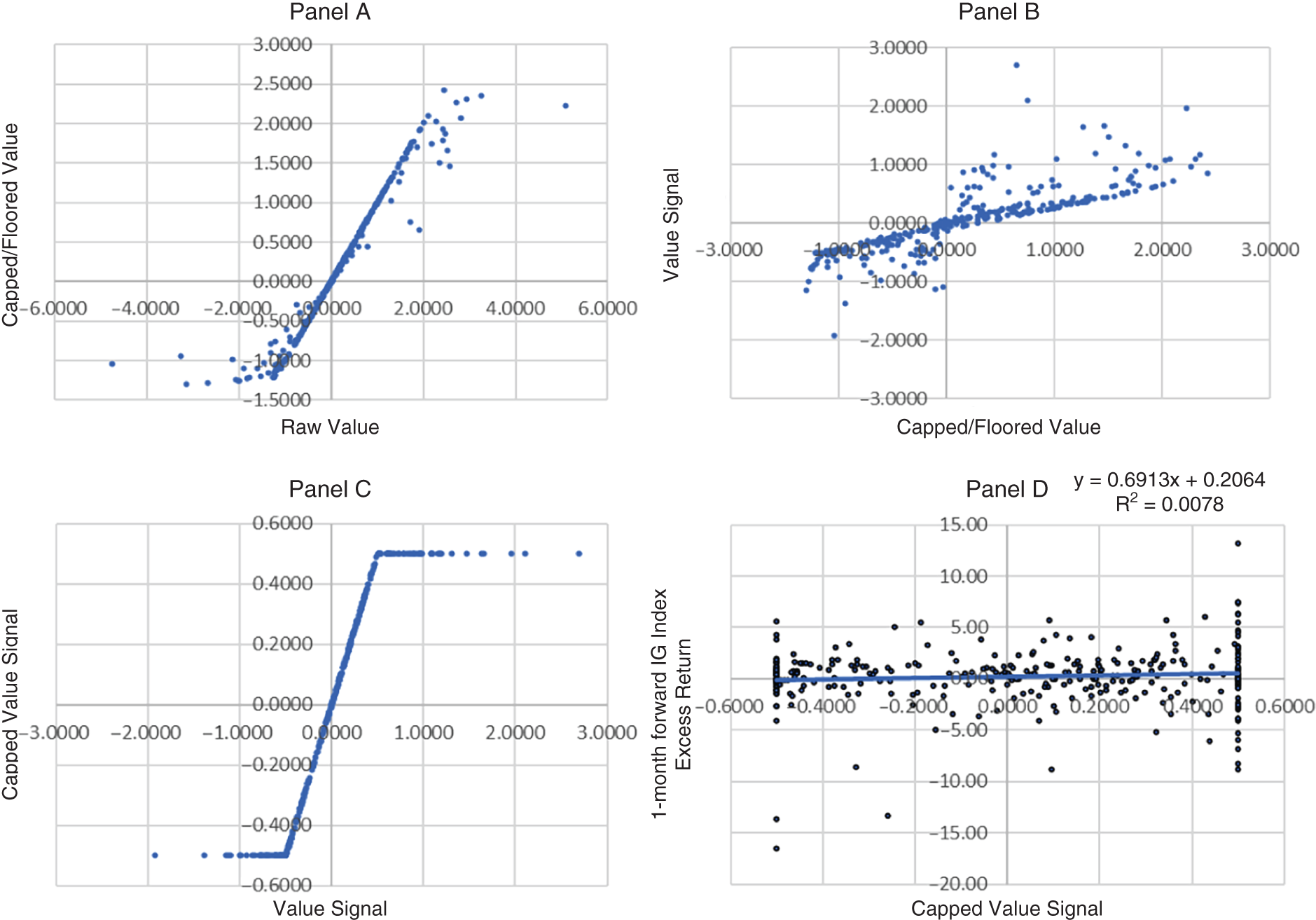
EXHIBIT 3.10 Value signals – Credit Premium (US HY). Panel A shows the effect of capping and flooring values at the 95th and 5th percentile (expanding window). Panel B shows the effect of benchmarking and volatility scaling (nonparametric Z‐scoring of the capped signal). Panel C shows the final signal‐timing curve. Panel D shows the link between value timing and one‐month‐ahead HY corporate bond index excess returns.
Sources: Described in text, period 1994–2020.

EXHIBIT 3.11 Momentum signals – Credit Premium (US HY). Panel A shows the effect of capping and flooring values at the 95th and 5th percentile (expanding window). Panel B shows the effect of benchmarking and volatility scaling (nonparametric Z‐scoring of the capped signal). Panel C shows the final signal‐timing curve. Panel D shows the link between momentum timing and one‐month‐ahead HY corporate bond index excess returns.
Sources: Described in text, period 1994–2020.

EXHIBIT 3.12 Carry signals – Credit Premium (US HY). Panel A shows the effect of capping and flooring values at the 95th and 5th percentile (expanding window). Panel B shows the effect of benchmarking and volatility scaling (non‐parametric Z‐scoring of the capped signal). Panel C shows the final signal‐timing curve. Panel D shows the link between carry timing and one‐month‐ahead HY corporate bond index excess returns.
Sources: Described in text, period 1994–2020.
EXHIBIT 3.13 Active returns from tactically timing credit premium (US IG Corporate Bonds).
| Momentum | Carry | Value | Value + Momentum | Value + Momentum + Carry | |
|---|---|---|---|---|---|
| Average | 0.02% | 0.27% | 0.01% | 0.01% | 0.10% |
| Std. Dev. | 0.0169 | 0.0179 | 0.0210 | 0.0081 | 0.0078 |
| Sharpe | 0.01 | 0.15 | 0.01 | 0.02 | 0.13 |
| Alpha (ann.) | 0.22% | 0.00% | −0.10% | 0.06% | 0.04% |
Sources: Described in text, period 1989–2020.
EXHIBIT 3.14 Active returns from tactically timing credit premium (US HY Corporate Bonds).
| Momentum | Carry | Value | Value + Momentum | Value + Momentum + Carry | |
|---|---|---|---|---|---|
| Average | 0.94% | 0.19% | 0.93% | 1.03% | 0.82% |
| Std. Dev. | 0.0387 | 0.0394 | 0.0398 | 0.0284 | 0.0169 |
| Sharpe | 0.24 | 0.05 | 0.23 | 0.36 | 0.48 |
| Alpha (ann.) | 1.73% | −0.79% | 0.83% | 1.37% | 0.71% |
Sources: Described in text, period 1994–2020.
The correlation across the active return series is informative to help understand the return profile of the combinations of signals. Value and momentum have a modest negative correlation of −0.33 (IG) and −0.02 (HY), value and carry have a modest positive correlation of 0.31 (IG) and 0.02 (HY), whereas momentum and carry have a very negative correlation of −0.85 (IG) and −0.86 (HY). This latter negative correlation is not surprising, because momentum tends to be positive when credit spreads have tightened relative to history (tightening spreads means positive credit excess returns), and carry is positive when credit spreads have widened relative to history. Of course, such a strong negative correlation raises questions about the efficacy of the selected measures. Indeed, more complete measures of carry that cover the entire shape of the credit curve, and broader measures of momentum, generate lower, but still negative correlations.
As with the term‐premium timing exercise, the combination of value and momentum, and value and momentum and carry, are formed by simple averages of the underlying fully transformed individual signals. Given their low pairwise correlations it is not surprising to see improved risk‐adjusted returns from the combinations. Again, this is diversification at work.
Although the Sharpe ratios are all positive, the magnitude is small especially for the IG market. The “alphas” are all very small in the IG market except for carry, but are much larger for the HY markets, especially for value and momentum. The caveat we stressed earlier about implementation costs and challenges is even more important for this market. Anyone planning to engage in timing the credit premium should understand the liquidity and trading costs. Credit index derivatives have become increasingly popular over the last 10 years, but the trading volumes are still small relative to equity index derivatives.
3.2.5 Skill in Timing
Exhibits 3.15 (IG) and 3.16 (HY) show the cumulative excess returns to a buy‐and‐hold position in corporate bonds (solid black line in each respective graph). The full tactical timing model that made equal use of value, momentum, and carry signals provides a useful addition, but only for HY markets (solid gray line). As with term premium timing, when we strip out the outperformance of each individual signal (dashed lines), the return potential is small relative to the passive exposure to the credit premium. Remember, “sin a little.”

EXHIBIT 3.15 Cumulative excess returns from US IG corporate bonds and associated tactical exposures.
Sources: Described in text, period 1994–2020.
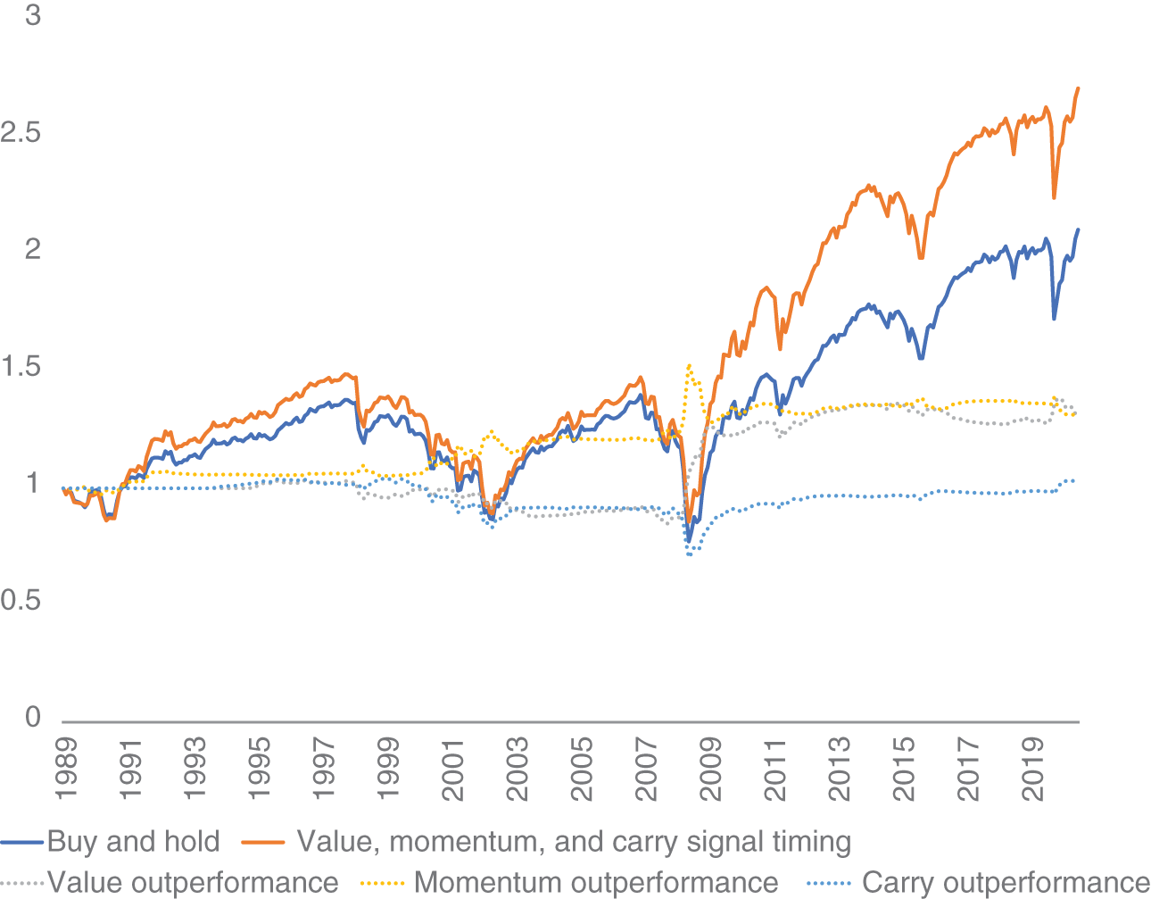
EXHIBIT 3.16 Cumulative excess returns from US HY corporate bonds and associated tactical exposures.
Sources: Described in text, period 1994–2020.
3.2.6 Extensions
Next, I discuss various avenues that asset owners and investors may wish to consider for their tactical investment decisions for the credit premium. The model developed in this chapter is far from exhaustive; there are many profitable extensions to explore. Carry measures can be enhanced by making full use of the credit term structure. Momentum can span price and fundamental measures. Our timing model only utilized price‐based momentum for the credit index itself, but price‐based measures of related assets (e.g., equity‐index returns) can also be examined. Fundamental measures can include changing expectations of firm level data (e.g., cash flows, operating profits, margins, etc.), and changing expectations of firm level defaults. This firm level data can be aggregated across companies in the index to form an index level view. Similarly, fundamental data can be sourced at the economy level directly. Corporate bond spreads are directly linked to economic growth expectations. Thus, measures of the real economy (industrial production, GDP, and aggregate employment) can be used as additional measures of momentum. Corporate bonds have a positive sensitivity to economic growth, so momentum in growth would be a positive signal for the credit premium.
Indeed, Asvanunt and Richardson (2017; AR), document that the credit risk premium varies with aspects of the business cycle. Using a growth composite based on the Chicago Fed National Activity Index and the “surprise” in the US industrial production growth, AR find that index‐level credit‐excess returns are higher in periods of economic growth. This is expected as companies benefit from overall economic growth, it will increase their ability to generate free cash flow that will, in turn, increase their asset value, thereby making them ‘safer’. Credit spreads naturally fall during periods of rising economic growth giving rise to positive credit‐excess returns. Using Moody's annual global default rates for investment grade bonds, AR construct a credit default composite of the year‐on‐year change in aggregate default rates and a measure of the surprise in aggregate default rates. Their surprise measure is the difference between the realized default rate over the 12‐month period relative to the Moody's Baa‐Aaa spread at the beginning of the period. AR find that credit excess returns are significantly higher during periods of lower default intensity. It is important to note that the analysis in AR is purely descriptive, because they were looking at measures of changing expectations of economic growth and default rates that are measured contemporaneously with credit‐excess returns. Investors looking to expand on their credit‐timing models should focus on business cycle forecasts and default intensity. We will have a lot to say about default modeling in Chapter 6.
Finally, on potential improvements to value metrics, a book could be written on the different approaches taken to explain credit spreads. As we will see in Chapter 6, the key determinant of credit spreads is expected loss given default (apologies for jumping ahead). Improved value metrics will focus on forecasting that directly: improved forecasts of default or credit migration and associated recovery rates.
3.3 OTHER CONSIDERATIONS
3.3.1 Dangers of Data Mining
Although the dangers of data mining and in‐sample fitting are relevant for all investors, and especially for systematic investors who rely on data for their investment decision‐making process, this risk is particularly important for timing models. As we saw in Sections 3.1 and 3.2, there is only one data series that is utilized to test the efficacy of a timing model. In the case of timing the term premium, we were fortunate to have nearly a century of data to work with. For timing the credit premium, we had less than three decades of data. This is a problem.
Although systematic investors may pride themselves on not explicitly engaging in data mining (i.e., not running hundreds of specifications to try and find the specification that worked best in sample) there are at least two areas where implicit data mining creeps into the analysis. First, there are many choices that need to be made once you chose a raw data attribute to be utilized in a model. For example, we used the real bond yield as a value signal for timing exposure to the term premium. This measure is the difference between the yield on the asset to be timed and a maturity matched inflation forecast. There are choices about where the data for inflation forecasts are sourced. If you use survey data, which survey provider do you use? Do you use the mean or median value across the forecasters covered by that provider? Do you want to equally weight forecasters (i.e., those who have more skill or whose forecasts are likely to contain newer information might be up weighted)? There are choices about how to convert a real bond yield at a point in time to a signal. In most cases, you subtract an historical benchmark value of your signal to identify the sign of your signal. But how is this done? Do you use rolling look‐back periods or expanding look‐back periods? Mean or median values to identify the benchmark? Equal weighting for all prior time periods or place more weight on the more recent history? Often, a signal is also scaled by a measure of volatility to identify the strength of the signal (e.g., you expect to see larger changes in values for your signal in more volatile time periods). Do you want to volatility scale your signal? If so, do you use a parametric or nonparametric method? How do you convert your transformed signal to a trading decision (i.e., what is the shape of your timing curve)? Although we consistently used a capped/floored linear curve, there are many other possibilities.
All these choices were made for both timing models in Sections 3.1 and 3.2. Were these the best choices or most easily defensible choices? Although they may not have been obvious at the time, you now know there is considerable room for different choices to be made across each dimension for each signal. Similar choices need to be made for each signal and further choices as to how to aggregate across signals. If you were to map this out, there would be a very large number of combinations. The impact of these choices individually is not likely to matter too much, but the choices can quickly compound differences. Indeed, in a recent paper, Kessler, Scherer, and Harries (2020) examine 3,168 alternative implementations of equity value strategies in the S&P 500 universe and find full‐sample Sharpe ratios vary between −0.10 and 0.78. Therein lies the data‐mining risk: out of a large set of feasible design choices, there is a risk of “fitting” to maximize an in‐sample result. This concern is relevant not only for timing models covered in this chapter, but also for the cross‐sectional relative‐value models that we will cover in Chapters 5–7. A potential remedy for this type of data‐mining risk is to ensure consistency in choices across the research effort. If choices are made on data sources that are relevant across different geographies or asset classes, use the same data source. If choices are made for timing models in different asset classes (e.g., lookback periods, volatility scaling, demeaning, etc.) ensure similar choices are made across individuals. This helps mitigate data‐mining risks.
Second, there is a somewhat unique data‐mining risk that comes with timing models – namely, memory. This is especially true for those who have been investing for a while. Such individuals will have a good memory of mistakes that were made in the past and/or data attributes that they wished they had access to back in time. The risk here is that attempts to improve timing models over time add elements into the model that were either not available back in time (e.g., new data were collected once people realized they were relevant and that data are then back‐filled) or if the data were available investors were not aware of them or utilizing them correctly. Back‐filling is a serious risk, because, arguably, the model is “cheating” with respect to knowledge of that data and their efficacy should be tested only after the data are genuinely available to an investor. Newfound awareness is also a risk, but perhaps that reflects your ability to identify useful information, albeit after the fact, and the risk is that the model tweak is only beneficial for one data point in the time series.
Another approach that is often used by systematic investors where there may be a concern about data quality is to build your model using data from one provider (e.g., you may use yields, spread, and historical return information from ICE/BAML) and then test the return performance using data from a different provider (e.g., you may use future excess returns from Bloomberg). This is a prudent way to help mitigate finding false positives.
3.3.2 Adding Breadth
Our analyses in Sections 3.1 and 3.2 were limited to considering one market – namely, the United States. This was a deliberate choice, as we have the longest series of data to test the efficacy of tactical models. Asset owners do not need to limit themselves to timing decisions in just the United States, nor for limiting the investment decision to just one asset (10‐year bonds in the case of term premium and US IG corporate bond index in the case of credit premium). There is a wide set of risk‐free assets across developed markets from which it is possible to express timing views on the relative attractiveness of the term premium. Similarly, there are multiple corporate bond indices from which it is possible to express timing views on the relative attractiveness of the credit premium. These tactical models could be extended to emerging markets as well. Although this can enhance the breadth of tactical allocation models, it is important to keep in mind that these are not independent bets, because there is a large common component in yield moves across countries and aggregate credit spreads across geographies and rating categories. Careful risk budgeting is needed to account for the correlated positions.
Expanding breadth for tactical investment decisions on term and credit premium also opens the choice of delta‐adjusting your investment views. For example, in the cross‐section of credit sensitive securities, there is natural variation in the sensitivity of the credit and equity claims for an issuer (see e.g., Lok and Richardson 2011). As the riskiness of the borrower increases (think of increased leverage and/or increased volatility), the credit claim starts to resemble the equity claim more closely (Schaefer and Strebulaev 2008). In options‐pricing language, the debt claim is more in the money and the value of that claim is more sensitive to the underlying asset value of the corporate issuer. Exhibit 3.17 shows this relation for a company that has both debt and equity outstanding. For simplicity, we assume that the risk‐free rate is zero, the firm does not pay dividends, asset volatility is 40 percent, and the outstanding debt has a value of $100. The hockey‐stick shaped lines capture the intrinsic value of the respective claim (i.e., the equity claim has an intrinsic value of zero when the value of assets is less than the amount that needs to be paid to creditors). The dashed and dotted curves reflect the market value of the debt and equity claims, respectively, using standard option pricing formulae.

EXHIBIT 3.17 Relation between credit and equity values and underlying asset value.
What can we learn from Exhibit 3.17? As you start at the far right of Exhibit 3.17, the asset value of the firm is far more than the outstanding debt. Thus, any change in the expected asset value has very minimal impact on the credit value (i.e., the slope of the upper dashed line is relatively flat, so the debt claim is out of the money). But as you move from right to left, the asset value decreases relative to the value of the outstanding debt (the “distance to default” decreases) and the sensitivity of the credit claim to underlying asset value increases. At the point where the asset value approaches the value of outstanding debt, the sensitivity of the credit claim to changes in asset value approaches the sensitivity of the equity claim to changes in asset value (i.e., the slope of the two dashed lines become more similar as you move toward the middle). This is the key take‐away: the credit and equity are expected to co‐move more strongly when there is more underlying credit risk (up to a point, of course, because in distressed situations the equity claim becomes insensitive to changes in asset values because it is too far out of the money).
What is the relevance to our tactical timing discussion? Investment decisions around aggregate credit markets might include views on (i) North American vs European corporate indices, (ii) IG vs. HY corporate indices, and (iii) developed vs. emerging market corporate indices. The set of issuers in the respective indices vary based on their underlying credit risk and, as such, the relevance of equity market information may be differentially important.
A similar line of reasoning can be applied to tactical investment decisions around the term premium. There are multiple liquid points across the yield curve in most developed markets. This provides additional breadth to capture attractive term premium at different points on risk‐free curves. Although the yield curve shares common exposure to current short‐term interest rates and the expected path of future short‐term interest rates, the sensitivity of longer‐term yields to expected central bank monetary policy actions, and recent news related to real economic growth (e.g., employment, GDP, industrial production, etc.) is less, so there is scope in tailoring investment decisions by utilizing differential sensitivity to fundamental information. This is true for both risk‐free and risky bonds.
3.3.3 Remaining Fully Invested
Let's finish this chapter with an important reminder of the bigger picture. All the analysis in this chapter was about varying your capital (or risk) allocation to fixed income assets based on forecasts of the conditional attractiveness of the term premium or credit premium. Therefore, at certain times you will be overinvested in government or corporate bonds and at other times you will be underinvested in government or corporate bonds. The determination of conditional attractiveness was made in a partial equilibrium framework with no direct awareness of what else was happening in the asset owner's overall portfolio.
Similar approaches for tactical timing can be applied to other asset classes, especially stocks. An asset owner needs to appreciate the consequences of tactical timing decisions in one asset class. How are these investment decisions to be funded? If the tactical insights are implemented via a derivative overlay, that may simply mean allowing risk levels to vary through time around a long‐term target. By itself, that may not be too challenging, but when there are multiple tactical timing decisions across asset classes (and even within asset classes as we have examined here with term and credit premia), what happens if tactical investment views across the board are suggesting to take more or less risk? As of writing in 2021, with interest rates low and elevated asset prices across most markets (public and private), this is a daunting challenge for asset owners. Although it might be easy to say government bonds look expensive, what else looks cheap where you may reallocate your capital (risk)?
REFERENCES
- Asness, C., A. Ilmanen, and T. Maloney. (2017). Market timing: Sin a little resolving the valuation timing puzzle. Journal of Investment Management, 15, 23–40.
- Asness, C., T. Moskowitz, and L. Pedersen. (2013). Value and momentum everywhere. Journal of Finance, 68, 929–985.
- Asvanunt, A., and S. Richardson. (2017). The credit risk premium. Journal of Fixed Income, 26, 6–24.
- Brooks, J. (2017). A half century of macro momentum. AQR working paper.
- Grinold, R., and R. Kahn. (2000). Active Portfolio Management. McGraw‐Hill.
- Houweling, P., and J. van Zundert. (2017). Factor investing in the corporate bond market. Financial Analysts Journal, 73, 100–115.
- Israel, R., D. Palhares, and S. Richardson. (2018). Common factors in corporate bond returns. Journal of Investment Management, 16, 17–46.
- Kessler, S., B. Scherer, and J. Harries. (2020). Value by design? Journal of Portfolio Management, 46, 25–43.
- Kozicki, S., and P. Tinsley. (2006). Survey‐based estimates of the term structure of expected US inflation. Bank of Canada, working paper.
- Lok, S., and S. Richardson. (2011). Credit markets and financial information. Review of Accounting Studies, 16, 487–500.
- Schaefer, S. M., and I. A. Strebulaev. (2008). Structural models of credit risk are useful: Evidence from hedge ratios on corporate bonds. Journal of Financial Economics, 90, 1–19.