
CHAPTER 11
Putting It All Together
OVERVIEW
Our final chapter is a short one. Our journey through the book started with a discussion of the size of fixed income markets and the (currently) small presence of systematic investors in fixed income. Might a systematic approach be successful? The book has introduced the various tools for modeling expected returns, risks, liquidity, and ultimately building portfolios in a systematic manner. A systematic approach could be successful. We also discussed how incumbent fixed income managers have, as a group, beaten their benchmarks, but have done so by leaning into traditional risk premia rather than security selection. In this chapter we will discuss how a well‐implemented systematic approach may beat a benchmark and do so not by loading up on traditional market risk premia, but, instead, via security selection opportunities. A well‐implemented systematic investment approach can be a powerful diversifier.
11.1 WHAT MIGHT A SUCCESSFUL SYSTEMATIC FIXED INCOME INVESTING PROCESS LOOK LIKE?
Let's examine the return properties of representative systematic fixed income portfolios. We will look at many of the active fixed income categories examined in Chapter 4. These portfolios are hypothetical representations of what might be possible from well‐implemented systematic portfolio construction (i.e., putting together everything we have discussed throughout the book). Revisiting the investment cube, this means mastery of the front face of the cube (breadth and depth of measures) and also of critical skills in implementation and portfolio construction. All strategy returns examined in this chapter are gross of any management fees but include estimates of transaction costs.
11.1.1 Investment Grade Corporate
A systematic long‐only (benchmark‐aware) IG corporate bond portfolio might select a global IG corporate bond index as its benchmark (e.g., Bloomberg Barclays Global Aggregate Corporate Total Return Index or ICE/BAML Global Corporate Bond Index). The systematic portfolio would select a level of active risk (tracking error that we discussed in Chapter 8) to offer investors (e.g., 1.0 percent). The amount of active risk is an investment choice and, as discussed in Chapter 8, it is a function of the volatility of the asset class itself (i.e., lower active risk for asset classes with less volatility) and parameters of your investment process (e.g., maximum position constraints at the issuer level may limit the total risk you are able to generate).
That active risk budget is then “spent” by the systematic investment process. It would include return forecasts spanning the various sources of returns (e.g., carry, defensive, momentum, value, sentiment, and other investment themes) covered in Chapter 6. It would seek to capture return potential in an idiosyncratic way identifying attractive issuers relative to a peer group (e.g., within industry) and attractive issues for a given issuer. The primary objective of the systematic investment process is to maximize the returns for the active risk taken. This is typically done while providing the beta of the benchmark. In the case of a global IG corporate bond portfolio, that beta includes a rate and a spread component across multiple currencies, so beta completion (covered at the end of Chapter 8) becomes an important part of the portfolio construction process. As you buy the most attractive corporate bonds based on your process, you need to keep track of the rate and spread exposure across countries, currencies, rating categories, industries, maturity buckets, etc. If done well, the final portfolio should isolate well‐compensated sources of idiosyncratic returns.
So, what might a systematic IG corporate bond portfolio look like? Exhibit 11.1 shows a scatter plot of the excess of benchmark returns for a systematic global IG corporate bond portfolio compared to the credit premium, ![]() (the same 50%/50% blend of Barclays U.S. High Yield Corporate Bond Index returns in excess of Duration‐Matched Treasuries, and S&P Leverage Loan Index in excess of three‐month LIBOR used in Chapter 4). This visualizes the following regression:
(the same 50%/50% blend of Barclays U.S. High Yield Corporate Bond Index returns in excess of Duration‐Matched Treasuries, and S&P Leverage Loan Index in excess of three‐month LIBOR used in Chapter 4). This visualizes the following regression:
It is clear there is no positive association between the excess of benchmark returns for the systematic IG corporate bond portfolio and the credit premium. The regression equation is reported in Exhibit 11.1 and the ![]() is very low (0.54 percent). The slope coefficient is negative (−0.0114) but not significantly so (t‐statistic of −1.08). The (annualized) intercept of 0.0097 and the (annualized) volatility of regression residuals (1.29 percent) suggest an information ratio (IR) of 0.75 for a systematic global IG corporate bond portfolio. If this systematic portfolio was run with an active risk of 100 basis points, this would translate to 75 basis points of alpha (0.75 × 1.0 percent). The IR is similar to the Sharpe ratio (0.71) due to the effort in portfolio construction where (i) all signals were built to be neutral to traditional market risk premia, and (ii) the optimization process, via constraints and completion, helped ensure the final portfolio had the greatest chance to provide alpha instead of beta.
is very low (0.54 percent). The slope coefficient is negative (−0.0114) but not significantly so (t‐statistic of −1.08). The (annualized) intercept of 0.0097 and the (annualized) volatility of regression residuals (1.29 percent) suggest an information ratio (IR) of 0.75 for a systematic global IG corporate bond portfolio. If this systematic portfolio was run with an active risk of 100 basis points, this would translate to 75 basis points of alpha (0.75 × 1.0 percent). The IR is similar to the Sharpe ratio (0.71) due to the effort in portfolio construction where (i) all signals were built to be neutral to traditional market risk premia, and (ii) the optimization process, via constraints and completion, helped ensure the final portfolio had the greatest chance to provide alpha instead of beta.
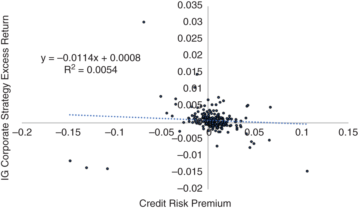
EXHIBIT 11.1 Scatter plot of excess of benchmark returns for a systematic IG corporate bond portfolio against the credit premium (50/50 blend of US HY credit‐excess returns and US Loan excess returns).
Sources: ICE/BAML indices, S&P indices, and author calculations. The period examined was 2003–2020.
11.1.2 Long Duration IG Corporate
Although this chapter is emphasizing the diversifying potential of systematic investment approaches, it is useful to remember the scalability of systematic investment processes generally. Long duration corporate bond mandates are a classic example. Public and corporate pension plans in North America have an almost insatiable appetite for long duration corporate bond portfolios. Pension plans have a desire to match expected future cash flows on their investments with expected future cash flows on their liabilities. Long‐dated corporate bonds issued in USD help fill this demand. It is an easy extension to tailor the global IG corporate bond portfolio to focus on USD long‐dated corporate bonds.
What might a systematic long‐duration IG corporate bond portfolio look like? A typical long‐duration corporate benchmark (e.g., Bloomberg US 10+ Year Corporate Bond Index or ICE/BAML 10+ Year US Corporate Index) will contain a smaller set of corporate issuers. This is because not all IG rated corporate issuers have bonds with more than 10 years of remaining maturity and, for those that do, only their longest bonds are eligible for the long‐duration benchmark. That said, there are still over 3,000 bonds in the typical long‐duration benchmark, which is more than enough opportunity to engage in security selection. The tracking error (active risk) for a long‐duration corporate bond portfolio is typically a little higher than a regular IG corporate bond portfolio (around 1.5 percent).
Exhibit 11.2 shows a scatter plot of the excess of benchmark returns for a systematic long duration IG corporate bond portfolio compared to the credit premium, ![]() . This visualizes the following regression:
. This visualizes the following regression:
It is clear there is no positive association between the excess of benchmark returns for the systematic long duration IG corporate bond portfolio and the credit premium. The regression equation is reported in Exhibit 11.2, and the ![]() is very low (1.13 percent) and the slope coefficient is negative (−0.0209) but not significantly so (t‐statistic of −1.69). The (annualized) intercept of 0.0118 and the (annualized) volatility of regression residuals (1.61 percent) suggest an information ratio of 0.73 for a systematic long‐duration IG corporate bond portfolio. If this systematic portfolio was run with an active risk of 100 basis points this would translate to 110 basis points of alpha (0.73 × 1.5 percent). Again, the IR is similar to the Sharpe ratio (0.69) due to the effort in portfolio construction where (i) all signals were built to be neutral to traditional market risk premia, and (ii) the optimization process, via constraints and completion, helped ensure the final portfolio had the greatest chance to provide alpha instead of beta.
is very low (1.13 percent) and the slope coefficient is negative (−0.0209) but not significantly so (t‐statistic of −1.69). The (annualized) intercept of 0.0118 and the (annualized) volatility of regression residuals (1.61 percent) suggest an information ratio of 0.73 for a systematic long‐duration IG corporate bond portfolio. If this systematic portfolio was run with an active risk of 100 basis points this would translate to 110 basis points of alpha (0.73 × 1.5 percent). Again, the IR is similar to the Sharpe ratio (0.69) due to the effort in portfolio construction where (i) all signals were built to be neutral to traditional market risk premia, and (ii) the optimization process, via constraints and completion, helped ensure the final portfolio had the greatest chance to provide alpha instead of beta.

EXHIBIT 11.2 Scatter plot of excess of benchmark returns for a systematic long‐duration IG corporate bond portfolio against the credit premium (50/50 blend of US HY credit‐excess returns and US Loan excess returns).
Sources: ICE/BAML indices, S&P indices, and author calculations. The period examined was 2000–2020.
11.1.3 HY Corporates
A systematic long‐only (benchmark‐aware) US HY corporate bonds portfolio might select the Bloomberg US Corporate High Yield Index or the ICE/BAML US High Yield Index as its benchmark. The choice of specific benchmark does not really matter and is typically a preference of the asset owner. The indices are typically very highly correlated, and while they do have differences (e.g., minimum face value, liquidity filters, issuer concentration limits, etc.), they are more similar than they are dissimilar. Compared to the IG corporate bond portfolios examined earlier, the amount of active risk for HY corporate bond portfolios tends to be closer to 2 percent.
Exhibit 11.3 shows a scatter plot of the excess of benchmark returns for a systematic US HY corporate bond portfolio compared to the credit premium, ![]() . This visualizes the following regression:
. This visualizes the following regression:
There is a small positive association between the excess of benchmark returns for the systematic US HY corporate bond portfolio and the credit premium. The regression equation is reported in Exhibit 11.3. The ![]() is very low (1.26 percent) and, although the slope coefficient is positive (0.0354), it is not significantly so (t‐statistic of 1.79). The (annualized) intercept of 0.0226 and the (annualized) volatility of regression residuals (2.58 percent) suggest an information ratio of 0.88 for a systematic US HY corporate bond portfolio. If this systematic portfolio was run with an active risk of 200 basis points, this would translate to 176 basis points of alpha (0.88 × 2.0%). Again, the information ratio is similar to the Sharpe ratio (0.91) due to the effort in portfolio construction where (i) all signals were built to be neutral to traditional market risk premia, and (ii) the optimization process, via constraints and completion, helped ensure the final portfolio had the greatest chance to provide alpha instead of beta.
is very low (1.26 percent) and, although the slope coefficient is positive (0.0354), it is not significantly so (t‐statistic of 1.79). The (annualized) intercept of 0.0226 and the (annualized) volatility of regression residuals (2.58 percent) suggest an information ratio of 0.88 for a systematic US HY corporate bond portfolio. If this systematic portfolio was run with an active risk of 200 basis points, this would translate to 176 basis points of alpha (0.88 × 2.0%). Again, the information ratio is similar to the Sharpe ratio (0.91) due to the effort in portfolio construction where (i) all signals were built to be neutral to traditional market risk premia, and (ii) the optimization process, via constraints and completion, helped ensure the final portfolio had the greatest chance to provide alpha instead of beta.
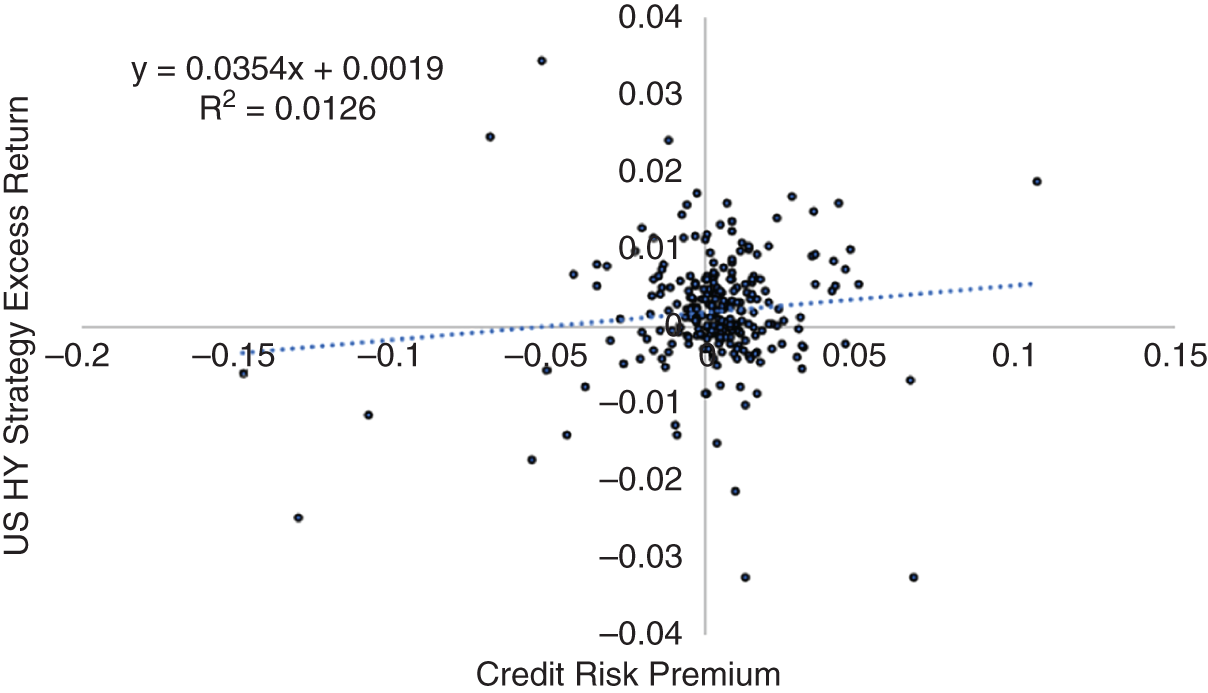
EXHIBIT 11.3 Scatter plot of excess of benchmark returns for a systematic US HY corporate bond portfolio against the credit premium (50/50 blend of US HY credit excess returns and US Loan excess returns).
Sources: ICE/BAML indices, S&P indices, and author calculations. The period examined was 2000–2020.
11.1.4 Credit Long/Short
A systematic approach to security selection can also be applied to a broader set of credit‐sensitive assets. Long/short implementations of single‐name corporate selection can be applied via derivatives (CDS contracts) and cash instruments in developed markets. Aggregate‐level credit risk could also be traded outright, as mentioned in Chapter 3. Investment decisions around aggregate credit markets might include views on (i) North American vs. European corporate indices, (ii) IG vs. HY corporate indices, (iii) developed vs. emerging market corporate indices, and (iv) credit curve positioning (e.g., 5‐year relative to 10‐year exposures). Capital structure approaches could also be applied at the corporate and index level, allowing for additional investment opportunities within the full spectrum of credit‐sensitive assets. The amount of active risk taken in long/short portfolios is much larger than that for benchmark‐aware portfolios (though the total risk of benchmark‐aware portfolios may be higher than long/short portfolios). The set of 51 credit long/short funds we examined in Chapter 4 had an average annualized return of 8.66 percent and a corresponding Sharpe ratio of 1.09, suggesting an active risk of around 9 percent for the current credit long/short manager. The systematic credit long/short portfolio that we will examine next will target an active risk of around 6–8 percent annually but importantly will seek to minimize exposure to traditional market risk premia.
What might a systematic credit long/short portfolio look like? Exhibit 11.4 shows a scatter plot of the excess of cash returns for a systematic credit long/short portfolio compared to the credit premium, ![]() . This visualizes the following regression:
. This visualizes the following regression:
There is a small positive association between the excess of cash returns for the systematic credit long/short portfolio and the credit premium. The regression equation is reported in Exhibit 11.4 and the ![]() is very low (0.93 percent) and, although the slope coefficient is positive (0.0945), it is not significantly so (t‐statistic of 1.34). The (annualized) intercept of 0.1069 and the (annualized) volatility of regression residuals (8.44 percent) suggest an information ratio of 1.27 for a systematic credit long/short portfolio. If this systematic portfolio was run with an active risk of 700 basis points, this would translate to 889 basis points of alpha (1.27 × 7.0 percent). The IR is similar to the Sharpe ratio (1.30) due to the effort in portfolio construction where (i) all signals were built to be neutral to traditional market risk premia, and (ii) the optimization process, via constraints and completion, helped ensure the final portfolio had the greatest chance to provide alpha instead of beta.
is very low (0.93 percent) and, although the slope coefficient is positive (0.0945), it is not significantly so (t‐statistic of 1.34). The (annualized) intercept of 0.1069 and the (annualized) volatility of regression residuals (8.44 percent) suggest an information ratio of 1.27 for a systematic credit long/short portfolio. If this systematic portfolio was run with an active risk of 700 basis points, this would translate to 889 basis points of alpha (1.27 × 7.0 percent). The IR is similar to the Sharpe ratio (1.30) due to the effort in portfolio construction where (i) all signals were built to be neutral to traditional market risk premia, and (ii) the optimization process, via constraints and completion, helped ensure the final portfolio had the greatest chance to provide alpha instead of beta.
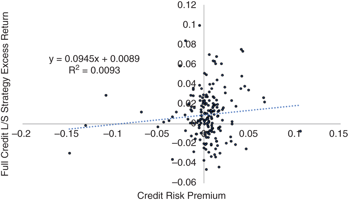
EXHIBIT 11.4 Scatter plot of excess of cash returns for a systematic credit long/short portfolio against the credit premium (50/50 blend of US HY credit excess returns and US Loan excess returns).
Sources: ICE/BAML indices, S&P indices, and author calculations. The period examined was 2004–2020.
The difference between a systematic credit long/short portfolio and the typical discretionary credit long/short fund examined in Chapter 4 is striking. Although all funds are run at similar levels of risk and are able to generate similar excess of cash returns (i.e., Sharpe ratios are above 1), there is a striking difference in the amount of beta packaged as alpha in this category. More than half of the excess of cash returns for the typical credit long/short fund is attributable to passive beta exposure. A systematic approach, in contrast, preserves its excess of cash returns after controlling for passive exposure to traditional market risk premia.
11.1.5 Emerging Markets
Emerging market fixed income covers a broad set of bonds: (i) local currency bonds issued by emerging sovereign, quasi‐sovereign, and corporate issuers, and (ii) hard currency bonds issued by emerging sovereign, quasi‐sovereign, and corporate issuers. A systematic approach can be applied to all these bond categories, but our focus here, as it was in Chapter 7, is on hard currency bonds issued by emerging sovereign and quasi‐sovereign entities.
Our systematic emerging market hard currency bond portfolio engages in security selection opportunities on both the country and maturity dimensions described in Chapter 7. The portfolio targets about 2 percent active risk (relative to the JP Morgan Emerging Market Global Diversified Index). This amount of risk is lower than the typical discretionary emerging market bond manager (Chapter 4 showed that the typical emerging market bond fund had a Sharpe ratio of 0.29 and average excess of benchmark return of 1.04 percent, suggesting a tracking error of around 3.5 percent).
What might a systematic emerging market bond portfolio look like? Exhibit 11.5 shows a scatter plot of the excess of benchmark returns for the systematic emerging market bond portfolio compared to the credit premium, ![]() . There is a small positive association between the excess of benchmark returns for the systematic emerging market bond portfolio and the credit premium. The regression equation is reported in Exhibit 11.5. The
. There is a small positive association between the excess of benchmark returns for the systematic emerging market bond portfolio and the credit premium. The regression equation is reported in Exhibit 11.5. The ![]() is very low (0.12 percent) and, although the slope coefficient is positive (0.0069), it is not significantly so (t‐statistic of 0.49). The (annualized) intercept of 0.0171 and the (annualized) volatility of regression residuals (1.68 percent) suggest an information ratio of 1.02 for a systematic emerging market bond portfolio. If this systematic portfolio was run with an active risk of 200 basis points, this would translate to 204 basis points of alpha (1.02 × 2.0 percent). The information ratio is similar to the Sharpe ratio (1.03) due to the effort in portfolio construction where (i) all signals were built to be neutral to traditional market risk premia, and (ii) the optimization process, via constraints and completion, helped ensure the final portfolio had the greatest chance to provide alpha instead of beta.
is very low (0.12 percent) and, although the slope coefficient is positive (0.0069), it is not significantly so (t‐statistic of 0.49). The (annualized) intercept of 0.0171 and the (annualized) volatility of regression residuals (1.68 percent) suggest an information ratio of 1.02 for a systematic emerging market bond portfolio. If this systematic portfolio was run with an active risk of 200 basis points, this would translate to 204 basis points of alpha (1.02 × 2.0 percent). The information ratio is similar to the Sharpe ratio (1.03) due to the effort in portfolio construction where (i) all signals were built to be neutral to traditional market risk premia, and (ii) the optimization process, via constraints and completion, helped ensure the final portfolio had the greatest chance to provide alpha instead of beta.

EXHIBIT 11.5 Scatter plot of excess of benchmark returns for a systematic emerging market bond portfolio against the credit premium (50/50 blend of US HY credit excess returns and US Loan excess returns).
Sources: JP Morgan indices, S&P indices, and author calculations. The period examined was 2004–2020.
To ensure fairness in the comparison to the set of 117 emerging market bond funds examined in Chapter 4, we can run the same regression specification:
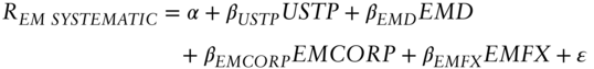
![]() is the monthly excess of benchmark return for the systematic emerging market bond fund, and the right‐hand side variables are all as defined in Exhibit 4.3. Exhibit 11.6 summarizes the regression analysis.
is the monthly excess of benchmark return for the systematic emerging market bond fund, and the right‐hand side variables are all as defined in Exhibit 4.3. Exhibit 11.6 summarizes the regression analysis.
The (annualized) intercept from regression 11.5 of 1.63 percent is marginally lower than the simpler analysis controlling only for the credit premium (note that the correlation to the credit premium, ![]() , is only 0.03). The information ratio, after adjusting for term premium, emerging premium, emerging credit premium, and emerging currency exposure, is 0.98. A well‐implemented systematic emerging market bond portfolio has the potential to be a powerful diversifier.
, is only 0.03). The information ratio, after adjusting for term premium, emerging premium, emerging credit premium, and emerging currency exposure, is 0.98. A well‐implemented systematic emerging market bond portfolio has the potential to be a powerful diversifier.
EXHIBIT 11.6 Regression analysis for systematic emerging market bond fund. Regression coefficients are reported on top of (italicized) t‐statistics.
| Active Return | Sharpe Ratio | IR | ||||||
|---|---|---|---|---|---|---|---|---|
| 1.74% | 1.03 | 0.07 | −0.06 | 0.05 | −0.03 | 1.63% | 0.98 | 0.03 |
| (2.10) | (−1.47) | (3.19) | (−1.19) | (13.63) |
Sources: Bloomberg indices, JP Morgan indices, and author calculations. The period examined was 2004–2020.
11.1.6 Global Aggregate and Unconstrained
The final systematic portfolio that we will evaluate in this chapter is one that combines security selection for rate and credit‐sensitive assets. We will explore these broad systematic fixed income portfolios in two ways. First, we will examine long‐only portfolios that use the Bloomberg Global Aggregate Index. Second, we will examine an alternative investment solution that takes active risk in an unconstrained benchmark agnostic manner. In both cases, the underlying systematic investment process is the same. Security selection for rate‐sensitive assets is expressed via country level and maturity views as described in Chapter 5. Security selection for credit‐sensitive assets is expressed across and within corporate issuer. Global fixed income portfolios also allow for active currency investment views to be incorporated. Although we have not focused on active currency management in this book, that is a commonly used additional lever for return enhancement on global fixed income portfolios. Finally, the unconstrained version allows for additional sources of return potential including tactical timing of the term and credit premium (as covered in Chapter 3) and extensions into emerging market bonds and HY corporate bonds (the “Plus” categories). The challenge will be whether a systematic approach can avoid the strong tendency of most existing active approaches in the unconstrained category to simply use the breadth enhancement as an excuse for more credit beta exposure. Can the additional breadth be harnessed in such a way to add security selection benefit without doubling down on credit beta?
A systematic Global Aggregate benchmarked portfolio could target about 1.5 percent of active risk, diversifying that active risk budget across credit‐sensitive asset security selection, rate‐sensitive asset security selection, and possibly active currency management. The systematic unconstrained portfolio (benchmarked to cash) could target a higher level of active risk (e.g., 4–5 percent annualized). This requires use of leverage, derivatives, and shorting to build positions that are large enough to offer attractive idiosyncratic returns. Consequently, a systematic unconstrained portfolio may not be for all asset owners (a levered strategy in the fixed income part of the asset owner's portfolio is not always the easiest sell). Let's examine how successful each portfolio might be.
Exhibit 11.7 shows a scatter plot of the excess of benchmark returns for a systematic Global Aggregate portfolio compared to the credit premium, CP. There is a small positive association between the excess of benchmark returns for the systematic Global Aggregate portfolio and the credit premium. The regression equation is reported in Exhibit 11.7. The ![]() is very low (1.23 percent) and, although the slope coefficient is positive (0.0148), it is not significantly so (t‐statistic of 1.63). The (annualized) intercept of 0.0101 and the (annualized) volatility of regression residuals (1.11 percent) suggest an information ratio of 0.91 for a systematic Global Aggregate portfolio. If this systematic portfolio was run with an active risk of 150 basis points, this would translate to 137 basis points of alpha (0.91 × 1.5 percent). The information ratio is similar to the Sharpe ratio (1.03) due to the effort in portfolio construction where (i) all signals were built to be neutral to traditional market risk premia, and (ii) the optimization process, via constraints and completion, helped ensure the final portfolio had the greatest chance to provide alpha instead of beta.
is very low (1.23 percent) and, although the slope coefficient is positive (0.0148), it is not significantly so (t‐statistic of 1.63). The (annualized) intercept of 0.0101 and the (annualized) volatility of regression residuals (1.11 percent) suggest an information ratio of 0.91 for a systematic Global Aggregate portfolio. If this systematic portfolio was run with an active risk of 150 basis points, this would translate to 137 basis points of alpha (0.91 × 1.5 percent). The information ratio is similar to the Sharpe ratio (1.03) due to the effort in portfolio construction where (i) all signals were built to be neutral to traditional market risk premia, and (ii) the optimization process, via constraints and completion, helped ensure the final portfolio had the greatest chance to provide alpha instead of beta.

EXHIBIT 11.7 Scatter plot of excess of benchmark returns for a systematic Global Aggregate portfolio against the credit premium (50/50 blend of US HY credit‐excess returns and US Loan excess returns).
Sources: ICE/BAML indices, S&P indices, and author calculations. The period examined was 2003–2020.
Again, to ensure fairness in the comparison to the set of 94 Global Aggregate funds examined in Chapter 4, we can run the same regression specification:

![]() is the monthly excess of benchmark return for the systematic Global Aggregate strategy, and the right‐hand side variables are all as defined in Exhibit 4.3. Exhibit 11.8 summarizes the regression analysis. The (annualized) intercept from regression 11.6 of 0.77 percent is lower than the simpler analysis controlling only for the credit premium (note that the correlation to the credit premium,
is the monthly excess of benchmark return for the systematic Global Aggregate strategy, and the right‐hand side variables are all as defined in Exhibit 4.3. Exhibit 11.8 summarizes the regression analysis. The (annualized) intercept from regression 11.6 of 0.77 percent is lower than the simpler analysis controlling only for the credit premium (note that the correlation to the credit premium, ![]() , is 0.11). The information ratio, after adjusting for term premium, credit premium, emerging premium, emerging currency exposure, and the volatility premium is 0.71. A well‐implemented systematic Global Aggregate portfolio has the potential to be a powerful diversifier.
, is 0.11). The information ratio, after adjusting for term premium, credit premium, emerging premium, emerging currency exposure, and the volatility premium is 0.71. A well‐implemented systematic Global Aggregate portfolio has the potential to be a powerful diversifier.
EXHIBIT 11.8 Regression analysis for systematic Global Aggregate strategy. Regression coefficients are reported on top of (italicized) t‐statistics.
| Active Return | Sharpe Ratio | IR | ||||||||
|---|---|---|---|---|---|---|---|---|---|---|
| 1.07% | 0.96 | 0.07 | 0.03 | −0.01 | 0.01 | 0.01 | 0.77% | 0.71 | 0.11 | |
| (2.36) | (1.26) | (−0.26) | (0.13) | (0.40) | (2.76) |
Sources: Bloomberg indices, JP Morgan indices, and author calculations. The period examined was 2003–2020.
Exhibit 11.9 shows a scatter plot of the excess of cash returns for a systematic Unconstrained Bond portfolio compared to the credit premium, CP. There is a positive association between the excess of cash returns for the systematic Unconstrained Bond portfolio and the credit premium. The regression equation is reported in Exhibit 11.9. The ![]() is a little higher than we have seen with other systematic strategies (6.58 percent) and the slope coefficient is positive (0.1612) and significant (t‐statistic of 4.20). Part of the unconstrained strategy includes a small capture of fixed income risk premia (inclusive of term premium, credit premium, emerging premium, and prepayment risk premium). Some exposure to traditional risk premia is expected in this category, and importantly, as we will see shortly, the extent of that traditional risk premia capture is small (especially compared to the incumbent Unconstrained Bond funds examined in Chapter 4) and it does not erode alpha. The (annualized) intercept of 0.0704 and the (annualized) volatility of regression residuals (5.00 percent) suggest an information ratio of 1.41 for a systematic Unconstrained Bond portfolio. If this systematic portfolio was run with an active risk of 500 basis points, this would translate to 705 basis points of alpha (1.41 × 5 percent).
is a little higher than we have seen with other systematic strategies (6.58 percent) and the slope coefficient is positive (0.1612) and significant (t‐statistic of 4.20). Part of the unconstrained strategy includes a small capture of fixed income risk premia (inclusive of term premium, credit premium, emerging premium, and prepayment risk premium). Some exposure to traditional risk premia is expected in this category, and importantly, as we will see shortly, the extent of that traditional risk premia capture is small (especially compared to the incumbent Unconstrained Bond funds examined in Chapter 4) and it does not erode alpha. The (annualized) intercept of 0.0704 and the (annualized) volatility of regression residuals (5.00 percent) suggest an information ratio of 1.41 for a systematic Unconstrained Bond portfolio. If this systematic portfolio was run with an active risk of 500 basis points, this would translate to 705 basis points of alpha (1.41 × 5 percent).

EXHIBIT 11.9 Scatter plot of excess of cash returns for a systematic Unconstrained Bond portfolio against the credit premium (50/50 blend of US HY credit‐excess returns and US Loan excess returns).
Sources: ICE/BAML indices, S&P indices, and author calculations. The period examined was 2000–2020.
Again, to ensure fairness in the comparison to the set of 103 Unconstrained Bond funds examined in Chapter 4, we can run the same regression specification:

![]() is the monthly excess of cash return for the systematic Unconstrained Bond strategy, and the right‐hand side variables are all as defined in Exhibit 4.3. Exhibit 11.10 summarizes the regression analysis. The (annualized) intercept from regression 11.7 of 3.99 percent is lower than the simpler analysis controlling only for the credit premium (the correlation to the credit premium,
is the monthly excess of cash return for the systematic Unconstrained Bond strategy, and the right‐hand side variables are all as defined in Exhibit 4.3. Exhibit 11.10 summarizes the regression analysis. The (annualized) intercept from regression 11.7 of 3.99 percent is lower than the simpler analysis controlling only for the credit premium (the correlation to the credit premium, ![]() , is 0.26), primarily due to the embedded capture of term premium and credit premium. The information ratio, after adjusting for term premium, credit premium, emerging premium, emerging currency exposure, and the volatility premium is 0.91. A well‐implemented systematic Unconstrained Bond portfolio has the potential to be a powerful diversifier.
, is 0.26), primarily due to the embedded capture of term premium and credit premium. The information ratio, after adjusting for term premium, credit premium, emerging premium, emerging currency exposure, and the volatility premium is 0.91. A well‐implemented systematic Unconstrained Bond portfolio has the potential to be a powerful diversifier.
EXHIBIT 11.10 Regression analysis for systematic Unconstrained Bond strategy. Regression coefficients are reported on top of (italicized) t‐statistics.
Sources: Bloomberg indices, JP Morgan indices, and author calculations. The period examined was 2000–2020.
| Active Return | Sharpe Ratio | IR | ||||||||
|---|---|---|---|---|---|---|---|---|---|---|
| 7.51% | 1.45 | 0.86 | −0.02 | 0.16 | −0.01 | 0.02 | 0.13 | 3.99% | 0.91 | 0.26 |
| (4.55) | (−0.20) | (2.73) | (−0.11) | (0.29) | (1.79) | (3.84) |
11.2 SOME FINAL THOUGHTS
I would like to close this book with some thoughts about careers in investment management, especially for systematic investors. This advice is largely parroting, perhaps not as eloquently, what I have been told over the past 20 years.
11.2.1 Failure Is Success
Anyone entertaining a career in systematic investments (fixed income or otherwise) needs to appreciate the importance of failure. A lot of investment ideas that you try will not work out as originally intended. This may not be because the idea had no merit, but, rather, the idea may not have been additive to what the investment process is already doing, or perhaps the market is more efficient with respect to your investment idea than you originally thought. Do not despair if the fruits of your effort only make marginal impact on the investment process in a given quarter or year. But do despair if someone working at a systematic investment business sets your key performance indicator to change the model by X percent. That is inconsistent with a systematic investment process. You should only take risk on an investment idea if it is conceptually grounded and empirically additive (see the recipe in Chapter 1). A systematic investment professional could have a very productive year yet have had minimal impact on the overall model.
Beware the hidden data‐mining risk in the research process. Although the famous quotes of Thomas Edison speak about not failing but finding thousands of ways that won't or don't work lend credence to the “fail and succeed” model, there is a serious risk of trying many things and focusing only on the positive results. This is an age‐old problem with all fields of research (not just investing). Keep track of the graveyard where all the failed ideas are buried. Not only is this good practice for efficient management of scarce investment resources (i.e., an idea that someone suggests today is usually related to an idea that someone else had tried years ago), it will also help the governance process. How many ideas or variants were examined? How robust are results across different, but defensible, research design choices? Absent knowledge of the graveyard, it is impossible to know how good a given research result is.
11.2.2 Culture Clash
Over the years, tensions between investment professionals (like any other workplace) need to be well managed. For a systematic investor, that means shared belief in the investment philosophy described in Chapter 1. At the same time, a good investment team needs individuals with a deep fundamental knowledge of the asset class (i.e., an ability to understand and model the return data‐generating process). It is unusual to find excellence in asset class domain knowledge and excellence in data analytics in the same individual. Herein lies the tension, as you need excellence across both dimensions to have a successful systematic investment process. And individuals typically want to be responsible for risk‐taking decision rights.
There are two potential solutions to this process. First, individuals can improve the dimension in which they are weaker (domain knowledge or data analytics skill). That is challenging, given the benefits of specialization and the limits of time. Second, the team can hire for excellence across dimensions. This is more common in practice. To be successful, however, individuals who join a systematic investment team should ensure expectations management are set both when they join and when their career develops. Exactly what skill set are you bringing to the table? How does your employer expect to utilize that skill set? Is that use consistent with what you are really passionate about? A similar thought process needs to be followed by the investment management company as well to ensure that the skill set acquired and the individual's career aspirations fit with the strategic plans. A lot of time and effort from both employee and employer are required to make an investment effort successful. It is a shame when there are expectations mismatches about roles and responsibilities.
Before starting a career in systematic investing, ask yourself what you really want to do. If it is the ability to have your own P&L and (ultimately discretionary) investment decision rights, then a career in collaborative systematic investing is not for you. There are differences in investment business models (for both systematic and discretionary processes) ranging from more collaborative efforts to more siloed and “eat what you kill” (smaller) teams. Systematic approaches can flourish across this spectrum. Think carefully what model is best suited for your personality.
11.2.3 Importance of Communication
Communication is an important part of success in all walks of life. For the systematic investor communication is, arguably, even more important than it is for a typical discretionary‐approach investor. Why? As we discussed in Chapter 1, a discretionary investment approach is characterized by a smaller number of positions with a clear narrative for each position in the portfolio. The discretionary portfolio manager is able to articulate the investment thesis for each key position in the portfolio. This “narrative” is important because it brings the asset owner into the investment process, and that shared understanding makes it easier to explain performance (both good and bad). A systematic portfolio manager, on the other hand, tends to find it challenging to provide a clear and compelling narrative for portfolio positions. Yes, this is a challenge, but it is a huge opportunity to bring your investors into the investment process. Simply stating that your systematic investment process seeks exposure to a set of characteristics like carry, defensive, momentum, and value, will work for some asset owners but not for all. How do you explain what you do to an asset owner if there are over 500 positions in the portfolio and all you have in front of you are four investment labels? An asset owner is going to want to know a lot more about the corporate bonds and government bonds in their portfolio. But that's okay. Leverage the power of data analytics to look through the portfolio positions down to the signals that gave rise to the positions (it is a deterministic process mapping data inputs to portfolio weights after all). There is considerable variety across systematic managers for portfolio attribution, and this is very much a nascent area. The successful systematic fixed investors will be those who are able to (i) generate positive excess of benchmark returns (a necessary condition for all investors), (ii) generate positive excess of benchmark returns that are lowly correlated with traditional risk premia (close to a sufficient condition), and (iii) clearly explain their investment process and provide deep levels of attribution to the portfolio.
The opportunity is there for systematic fixed income investors. As we noted in Chapter 1, only a very small portion of active fixed income funds are managed in a systematic way. The first section of this chapter showed how a systematic investment approach can be very different from, and very diversifying to, traditional discretionary fixed income managers. Part of that difference stems from lower exposure to traditional market risk premia, but part of that difference is also attributable to a different approach to security selection and portfolio construction. Palhares and Richardson (2020) explore the differences in discretionary and systematic investment approaches in the US HY market. That subgroup of fixed income managers is selected due to disclosure of portfolio holdings and the relative homogeneity across funds. The majority of US HY mutual‐fund corporate bond funds hold HY corporate bonds, and every quarter they disclose their holdings and their benchmark. It is easy to compute an active view for every corporate issuer and issue in that benchmark. The systematic corporate bond manager has an expected return forecast for every bond in the index. A heuristic similarity measure (labeled TC in Exhibit 11.11) can be computed for every fund quarter. The correlation between active weights and standardized values of the respective investment themes (carry, defensive, momentum, and value) is an efficient way to capture this similarity. It should be clear from Exhibit 11.11 that across the set of 154 HY mutual funds there is little similarity in active risk taking with a systematic investment approach. The vertical line toward the middle of each histogram is the average TC across mutual funds (it is close to zero as the market clears and the set of mutual funds is representative of the overall market).The vertical line at the right reflects the correlation for a systematic fund designed to target exposure to these four investment themes. It is very far to the right of the distribution of discretionary HY bond funds. A systematic investment approach can be a powerful diversifier
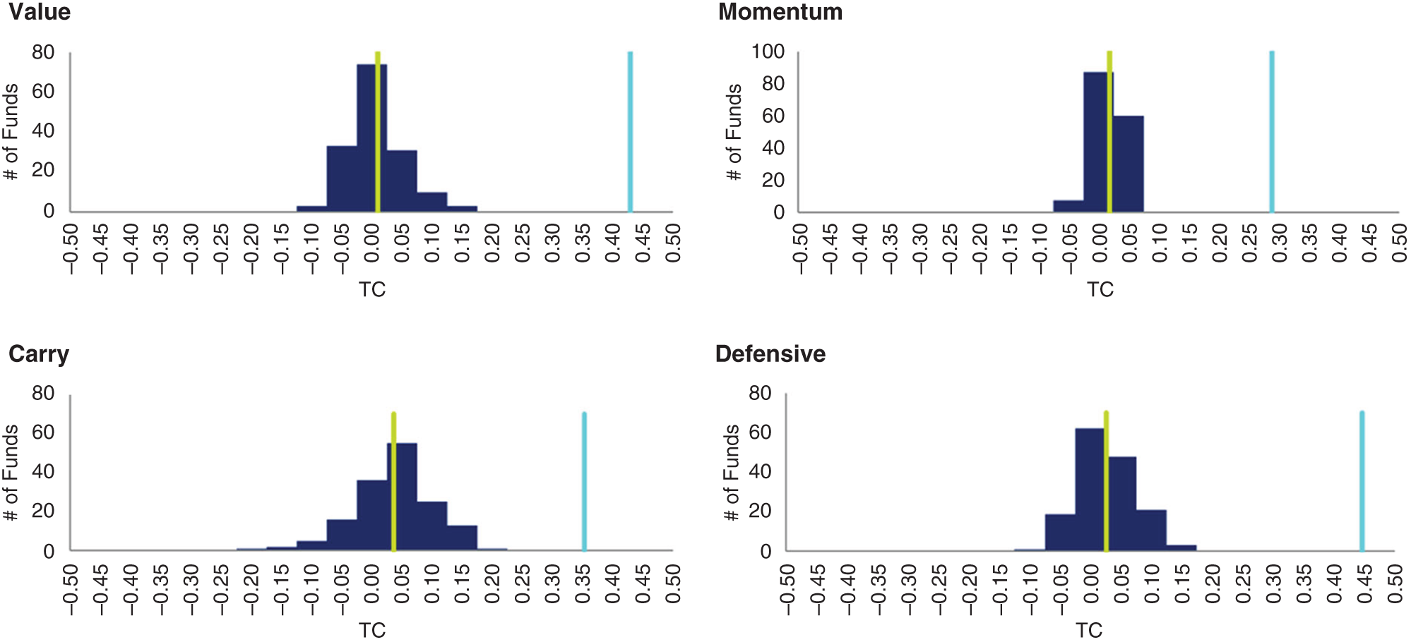
EXHIBIT 11.11 Holdings analysis of discretionary and systematic HY corporate bond managers. The charts show a relative frequency histogram of the transfer coefficient (TC) between fund active weights and standardized systematic measures of bond attractiveness for a set of 154 HY mutual funds. The light vertical line is the average TC across all mutual funds. The dark vertical line is the TC for a systematic HY bond portfolio.
Source: Palhares and Richardson (2020).
11.2.4 Market Efficiency
One final note. Be humble. A career in active investing requires you to challenge market prices. This is a daunting challenge. There is an enormous amount of capital invested in the markets every day. What is your edge? How can you maintain your edge? Always strive to articulate your investment thesis. Does a given measure associate with future returns due to (i) risk, (ii) behavioral/cognitive errors, or (iii) are you exploiting an institutional friction? Anything anchored on (ii) or (iii) should be continually challenged. Is your idea still not fully appreciated by the market? Is the friction still strong enough to be exploited? But note that just because something did not work recently is not, by itself, grounds for dismissing the efficacy of your idea.
Be sure you sleep soundly at night. Your belief in market efficiency should be consistent with (i) your investment career choice, and (ii) your personal investing decisions. A die‐hard believer in efficient markets should not be working in active investment management and should have all their financial assets with Vanguard. I wish you all the best in your systematic fixed income investing career. Together let's make the systematic share of actively managed fixed income strategies much larger. It will be good for you, and, most importantly, it will be good for your asset owners!
REFERENCE
- Palhares, D., and S. Richardson. (2020). Looking under the hood of active credit managers. Financial Analysts Journal, 76, 82–102.