
CHAPTER 8
Portfolio Construction Considerations
OVERVIEW
This chapter describes the portfolio construction process. There are many decisions that need to be made to convert your “signals” into portfolio positions. A successful systematic investment process needs to be excellent across many dimensions. These dimensions include: (i) breadth of investment themes covered, (ii) depth of measures across investment themes, (iii) choices in combining multiple investment themes and converting them to an expected return forecast, (iv) identifying a suitable set of fixed income securities that are appropriate for a systematic investment process (liquidity screening), (v) tracking error and risk modeling generally, and (vi) selecting sensible constraints to maximize risk‐adjusted returns while avoiding poorly compensated exposures. At the end of the chapter the reader should have a full appreciation of the challenges of portfolio construction, and hence understand the opportunity for skillful portfolio craftsmanship to improve the investor experience.
8.1 CHOICES IN THE INVESTMENT PROCESS (DESIGN AND INVESTMENT UNIVERSE)
Exhibit 8.1 is a simple visualization of the necessary ingredients for a successful investment process. There is nothing here that is specific to a systematic investment process since all aspects need to be implemented well for investment success for any investor. The previous three chapters have focused on Step 2 in the investment process: How do we rank the relative attractiveness of our assets? We now need to think more holistically about portfolio construction. Let's walk through each step and highlight the many choices that need to be made by the systematic investor along the way.
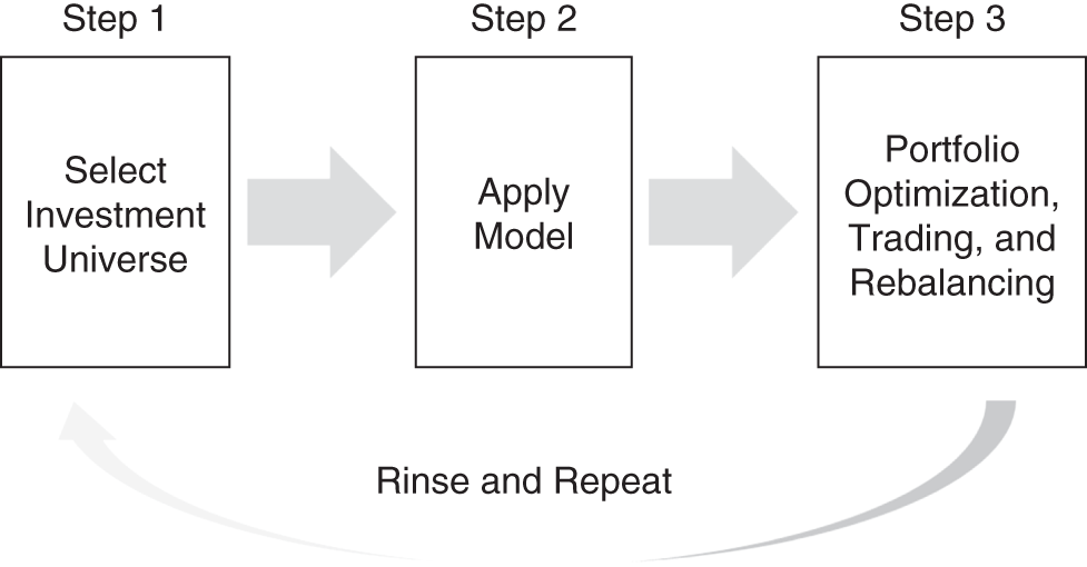
EXHIBIT 8.1 Visualization of the systematic investment process.
The first step in any investment process is defining the sandbox of eligible securities. In the case of comingled investment vehicles (e.g., US mutual funds formed under the Investment Company Act of 1940, or European‐domiciled UCITS funds [UCITS is short for Undertakings for the Collective Investment in Transferable Securities]), the prospectus that underlies the investment vehicle will contain the specific details of what is an eligible security. In the case of separately managed accounts there will be a formal document containing the investment guidelines that specify what the asset manager can and cannot do. The investment guidelines will typically specify a benchmark. For long‐only portfolios this is your starting point for eligible securities. The guidelines may then allow for out of benchmark securities that meet certain criteria (e.g., an IG corporate bond mandate may allow for a certain percentage of fund assets to be invested in non‐IG rated corporate bonds). For long–short unconstrained portfolios the benchmark is typically a cash rate (e.g., LIBOR or the new bank reference rates such as SONIA), and the investment guidelines will then specify the type of securities allowed in the investment vehicle.
Let's try to make this more concrete as we walk through the portfolio construction choices in this chapter. We will use credit‐sensitive assets as our working example for this chapter, but note that these choices need to be made for all fixed income securities (e.g., a Global Aggregate Index benchmarked portfolios will need to make choices on government bonds, corporate bonds and securitized assets). Our asset owner has decided to make an allocation to the US HY corporate bond market. They have selected the ICE/BAML H0A0 index as their policy benchmark for this asset allocation. As of December 31, 2020, the H0A0 index had 2,003 corporate bonds. Not all these bonds are suitable for the systematic investment process. Let's walk through some important dimensions that the investor needs to consider.
- Liquidity
A necessary condition for a successful systematic investment process is your ability to buy and sell assets in a cost‐effective way. It is no use modeling the attractiveness of an asset if it has not been traded for the past six months. I wish you all the best for discussions with your trading execution team if you keep modeling illiquid securities: they will never be able to buy the assets that you think are attractive, and you will keep telling them to look – not a recipe for success. Instead, a reasonable alternative is to prescreen your eligible universe based on “liquidity.” Yes, you will exclude the less liquid assets, but this does not come with a loss in expected return, as was discussed in Chapter 6 there is no evidence of a liquidity premium for public corporate bond markets.
How might you identify those bonds with less liquidity? Corporate bonds (government bonds, too, for that matter) do not trade on a centralized exchange. Consequently, it can be challenging to get reliable, comprehensive data on trading activity of individual bonds. Absent data it is not possible to identify whether a bond is liquid or not. So where might we source data on liquidity? In the United States, the TRACE engine provides sufficient data to be able to compute a variety of measures related to liquidity (e.g., fraction of no trading days, dollar volume traded, turnover, bid‐ask spreads, and market impact as measured in Palhares and Richardson 2019). Relationships with broker‐dealers can allow for aggregation of indicative quotes to get a sense for potential live bid‐ask spreads, depth, and frequency of market making opportunities. Aggregating across these data sources will allow you to remove from your investment universe bonds that are insufficiently liquid (exclusion). Some of this data will also be important later in the chapter when we discuss optimization and objective functions. Modeling expected transaction costs, inclusive of market impact, can be part of the systematic process. Likewise, trade size and position size constraints should also be liquidity aware (i.e., you should be able to trade large sizes and build larger positions for more liquid bonds).
- Seniority
Corporate bond indices will contain significant variability in seniority ranging from senior secured to unsecured to junior bonds. I have seen some investment approaches remove bonds that are too senior (e.g., secured) or too junior in the capital structure to help improve cross‐sectional comparability of eligible bonds. If the investor retains bonds that span the entire capital structure, careful attention should be given to forecasts of expected returns, especially for measures that are based on credit spreads (carry and value investment signals especially). All else being equal, seniority affects spreads directly through expected recovery rates. At a minimum, adjustments need to be made for expected recovery rates to ensure cross‐sectional comparability for value and carry signals.
- Remaining Time to Maturity
As we will see in Chapter 9, trading is operationally challenging and very costly relative to the return potential for credit‐sensitive assets. This has a direct impact on the optimal amount of turnover for a portfolio. A good investor will look to ration their turnover budget very carefully. You want to be buying bonds that you think have the highest expected return potential from your set of eligible securities and then selling bonds from your portfolio that have the least attractive expected return potential. As we discussed in Chapter 1, fixed income assets have a natural life; they die when they mature. It may therefore be rational to limit your enthusiasm for buying bonds that have the shortest duration or, at a minimum, do not force trading out of a bond as it exits an index or gets close to exit based on declining maturity. This would be a suboptimal use of your scarce turnover budget.
- Private Issuers
As discussed in Chapter 6, there are many private issuers in the corporate bond markets. As of December 31, 2020, 29 percent of the US HY index is comprised of private issuers. These are corporate entities for which it is more difficult to source relevant information to generate expected return forecasts. Does the systematic investor want to keep private issuers? If yes, should you entertain a minimum information threshold for retention in the investment universe? If you are not able to source sufficient information you will not be able to create an expected return forecast, so how can you include such assets in your portfolio? Excluding all private issuers is too extreme, but requiring a minimal information threshold is not.
- Domicile of Issuer
Attention needs to be paid to the domicile of the corporate issuer. In some cases, you will have corporate issuers who have issued in USD, but they are domiciled in emerging markets. Do you want to keep these issuers in the investment universe? Ideally, you want to increase the homogeneity of corporate issuers to increase your ability to identify relative value opportunities in the cross‐section.
Once you have made decisions on these dimensions, it is important to then understand how different your eligible universe is relative to the starting benchmark of securities. While you may have a sound basis for excluding securities, this set of excluded securities introduces what is called “tracking error” to your portfolio process. Formally, tracking error is a statistical measure of distance. How different is the performance of one portfolio from another? We had discussed tracking error earlier (Chapter 4) as an ex post return attribute (i.e., what was the volatility of the excess of benchmark returns). Here we are talking about tracking error from an ex ante perspective. Given a set of exclusions how different is your eligible security universe from the starting benchmark? The measure of difference is weighted by the riskiness of each security. For credit sensitive assets, as was discussed in Chapter 6, DTS (the product of spread duration and credit spread) is a useful proxy for risk. Let's assume you either exclude (i) a corporate bond (A) that has 1 percent weight in the benchmark and a DTS of 2,240 (a credit spread of 560 and spread duration of four years), or (ii) a corporate bond (B) that has 1 percent weight in the benchmark and a DTS of 5,550 (a credit spread of 1,850 and spread duration of three years). Both bonds have the same weight in the benchmark (i.e., you would exclude 1 percent of the benchmark in both cases), but they have a very different risk profile – B is riskier than A. Tracking error captures the difference in risk across the portfolios, which is a function of the weight of an asset and its contribution to risk (return volatility and correlation structure). This discussion is related to the topic of active share that we briefly discussed in Chapter 1. Simple differences in portfolio weights are a poor measure of distance between two portfolios. This limitation becomes more problematic as the degree of heterogeneity in risk in the cross‐section increases. And in the corporate bond universe, both IG and HY have very significant differences in risk contributions across index constituents.
The tracking error implications of investment universe exclusions need to be measured and monitored. We will come back to this later in the chapter when we discussion optimization and objective functions. Constraints are typically added to the objective function to limit the amount of active risk that is allowed on certain dimensions that you think are not well compensated (i.e., dimensions that are not part of your investment view). Examples might include maturity categories, rating categories, or industry groups that your exclusions affect, but for which you do not have an explicit view on expected return potential. So, it may then be prudent to limit the amount of active risk you take across those dimensions.
8.2 CHOICES IN THE INVESTMENT MODEL (EXPECTED RETURNS)
8.2.1 Which Investment Signals?
The prior three chapters introduced investment frameworks for government bonds, corporate bonds, and emerging market hard currency bonds specifically. There was overlap in the investment themes across these three types of fixed income assets (carry, defensive, momentum, and value themes). We focused on those themes, and simple measures of those themes, not because I believe only in simple measures of these themes, but to help lift the veil on systematic investment processes. You are not limited to these measures. Exhibit 8.2 is a simple visual of the potentially rich set of investment signals that could be part of your forecasted expected returns. Our focus here is the face of the cube that spans breadth and depth across potential investment themes. The usual suspects of carry, defensive, momentum and valuation investment themes are covered on the vertical axis, but additional investment themes like sentiment, smart money, liquidity provision, and so forth, could also be incorporated (the arrow suggests the potential for additional investment insights: that's the research process!)
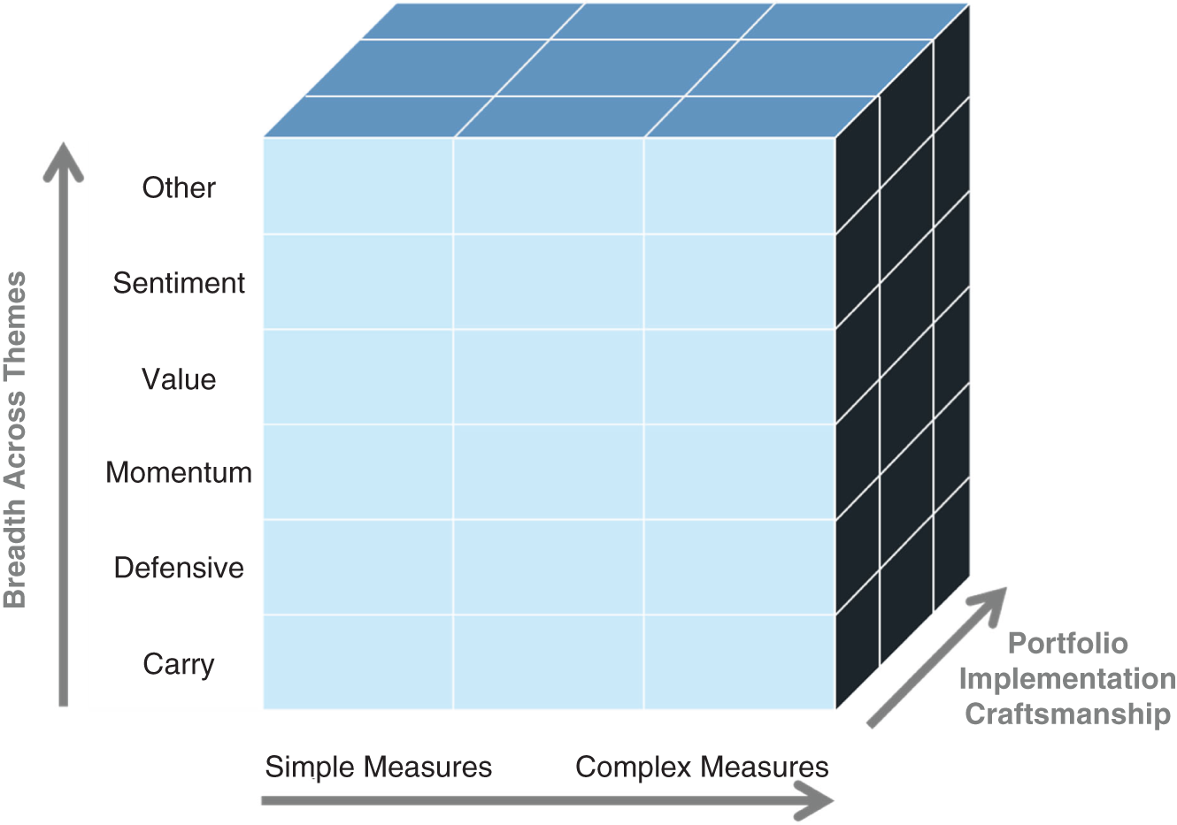
EXHIBIT 8.2 Visualization of the investment model (the investment cube).
Moving across the face of the cube we can add measures of the same investment theme. For example, as we discussed in the prior three chapters measures of momentum can include the asset's own price returns (simple) but can be extended to include measures of related asset returns and a variety of fundamental based momentum measures (complex). Likewise, measures of valuation can range from linear projections of spreads onto credit ratings and return volatility (simple), to structural models and nonlinear machine learning models (complex). It is not the pursuit of complexity alone that is of interest; depth of measures is only useful if they are conceptually additive to your investment process combined with data‐based evidence that more complicated measures improve your investment process. Again, the arrow continues to the right (the research process should be continually looking for improvements to existing investment themes). The front face of this investment cube can be useful to distinguish different types of systematic investment processes. Smart beta approaches would cover only the left portion of the face of the cube, and a full systematic investment process would span the entire face and would be looking to increase the size of the front face.
8.2.2 How to Group Investment Signals Together?
In most cases it is clear which signals belong together. Momentum measures are all related to recent performance (price and fundamental versions). Value measures all share similarities in that they compare yields (rate‐sensitive assets) or spreads (credit‐sensitive assets) to various fundamental anchors. Defensive measures capture measures of low risk or issuer quality. In these cases, economic priors should guide how signals are grouped together. There will, however, be instances where it is not clear how to combine themes together. Do you keep creating new investment themes as new signals are added? In the interest of parsimony, I recommend grouping signals together based on conceptual priors, and supplementing this with statistical analysis that examines how signals are correlated with each other and how the returns linked to signals are correlated with each other (the higher the correlation the more likely you are to group signals together).
Why is grouping signals together important? I view signal grouping as a precursor decision before the signal weighting decision. You could feed all of your signals into a signal weighting algorithm, but I think that is asking too much of the algorithm with too little data.
8.2.3 How to Select Weights for Investment Signals?
Given the prior discussion, there are at least two dimensions of signal‐weighting choices. First, for the signals you have grouped together, you need to allocate weights across the signals. I prefer an equal‐weighted allocation here unless you have strong conviction. That conviction could come from (relatively) unique data access for a given theme and/or (relatively) unique methodology to convert that data into a signal. For example, within valuation you may allocate a little more weight to the signals that make use of a larger set of fundamental information.
Second, you need to allocate weights across the signal groups. Again, I suggest strongly that you lean on priors here. Start with equal weighting across signal themes and deviate only in two cases: (i) if you have strong conviction of the efficacy of one signal group perhaps based on the depth of insights and number of measures allocate more weight, and (ii) if certain themes are slightly or negatively correlated with each other you will want to increase weights to these signals to help ensure they still matter at the aggregated level. There is a related conceptual topic here about signal correlation: make sure you understand the economic sources of correlation structure across signal categories. As we will see later in this chapter, choices are made to transform raw signals into return forecasts that can affect correlations. Check to make sure your transformations are improving your ability to combine information and not hindering that effort.
The astute reader will notice that I have said nothing about recent performance as the basis for selecting signal weights. As we saw in Chapter 3, tactical investment decisions (timing) is difficult to do successfully at the asset class level. It is also difficult to do well within an asset class across subgroups of assets. These subgroups could be industry groups or factor‐mimicking portfolios that target signals. The forecasting challenge is a significant reduction in investment breadth when you move from security selection across the entire eligible investment universe to a small number of subgroups (see, e.g., Grinold and Kahn 2000). Recent signal performance would be a way to “time” your risk allocation across signals (or factors). The topic of factor timing is a large one for asset managers and academics alike (see, e.g., Gupta and Kelly 2019 and references therein). If you are willing to entertain time variation in your weighting across signals, then looking at recent performance is certainly a potential way to do that. I would, however, caution enthusiasm. The evidence for factor timing to date has been in the context of equity markets where it is relatively easier (and cheaper) to trade. So what may look like a modest improvement in risk‐adjusted returns for an academic portfolio that ignores real‐world implementation challenges may be anything but. Your turnover budget is scarce. Use it on the highest expected return opportunities. I'm not sure factor timing meets that hurdle.
Two final comments on factor timing: valuation and diversification. I have lost count of the number of times that asset owners have suggested that an investment theme has become too expensive and as such you should reduce your weight to that theme (the defensive theme in equity has been a common example for several years). Although that observation and suggested investment decision may have merit, what it fails to fully appreciate is that an investment approach that allocates risk across valuation and other themes is already endogenously timing exposure to other themes based on their prevailing valuation (i.e., the correlation between signals is dynamic and that will be reflected in the final portfolio that maintains strategic weights across investment themes). So, you are getting some value timing for free in a diversified systematic investment approach. Finally, diversification itself is the free lunch that we can risk forgetting at our expense. If your decision to time vary weights across investment themes has a low success rate you will lose the benefit of diversification (i.e., when one of them performs below average another theme is likely to perform above average, it is just hard to tell ex ante which theme will under‐ or overperform).
My overall recommendation here is to think carefully about factor timing, especially for the more expensive credit sensitive assets. And be wary of commercial vendors offering timing products when their commercial interest is really driven by increased trading activities.
8.2.4 What Units Are These Weights In?
Implicit in all the previous discussion about signal weighting is that we are allocating 100 percent of our signal weights to each investment theme. But 100 percent of what? The systematic investment process is designed to deliver attractive risk adjusted returns. Typically, you are trying to maximize your information ratio, the ratio of excess of benchmark (beta‐adjusted) returns scaled by a measure of ex‐ante active risk. The denominator of the information ratio (active risk) is the units we are allocating signal weights from. You can think of a risk budget for your investment strategy. For a HY corporate bond portfolio, that might be 2 percent annualized, for an IG corporate bond portfolio that might be 1 percent, and for a long‐duration IG corporate bond portfolio that might be 1.5–2 percent. The amount of active risk taken for a given investment vehicle is also an investment choice. Generally, the amount of active risk scales with the risk of the underlying asset class (i.e., an equity portfolio will have more active risk than a core fixed income portfolio).
Signal weighting is typically done in risk terms. If you have a 2 percent active risk budget and are deciding how much (risk) weight to allocate to four investment themes, those weights should be applied to portfolios formed on each investment signal where the weights have been adjusted to allow for comparability across investment themes. Consider carry as an investment theme. Your carry long/short portfolio, like that examined in Chapter 6, would have the long and short side of the portfolio equal each other in dollar terms (i.e., be dollar‐neutral), but it will be a very imbalanced portfolio in terms of market exposure and it will have more risk than a similar portfolio formed on another theme (say defensive). How to adjust the portfolios to improve comparability? The portfolio weights can be scaled up or down to target a specific level of volatility. This requires a measure of risk, which could be as simple as DTS or could be a more advanced common factor risk model (more on that later in the chapter).
8.2.5 Could/Should You Vary Active Risk Through Time?
Separate from the strategic versus tactical weighting decision across signals (e.g., the choice to increase or decrease your exposure to a certain signal due to recent performance), there is a related decision on whether to allow the aggregate amount of active risk to vary through time or not. This may not be immediately obvious the first time you are asked this. What causes temporal variation in active risk across a combination of investment themes if I am targeting a fixed set of risk weights across the set of investment themes? The individual thematic portfolios may take the same amount of risk at each point in time, but the combination is not guaranteed to do so because of time varying correlation structures across the investment themes. At certain times, signals will be more positively correlated to each other. At certain times, some themes will like a similar set of securities. When this happens, the aggregate active risk across themes will be greater. This is your choice: Do you want to allow that time variation of active risk in your investment process or not? If you believe that risk‐adjusted returns are stronger when there is greater agreement across investment themes, then allow that time variation in active risk.
8.2.6 Signal‐Specific Investment Choices
- Ordinal/Cardinal: Although each signal has a natural unit, do you want to keep that natural scale (cardinal) or are you mostly interested in the rank ordering across bonds (ordinal)? Perhaps you want to use both dimensions.
- Missing values: How do you want to treat missing values? Excluding bonds with missing values will be very restrictive, especially when you are integrating across many signals. If you have no information for a given signal this is equivalent to a neutral view. Assigning a neutral value may be appropriate. But note that zero is not necessarily a neutral value. It all depends on the scale of the signal and any other treatment you have made to the signal (e.g., group demeaning). In class assignments this choice perplexes students as they can make the neutral value (zero) replacement too early in the process. For example, if your signal was leverage (preference for corporate issuers with lower leverage) then if you assign a value of zero for firms where you could not measure leverage (say private issuers where you are unable to source financial statement data), that choice means you maximally like firms with missing data to compute leverage. I doubt that was your investment view. Alternative treatment for missing values could be imputation based on available data for similar firms (we will see an example of this in Chapter 10 for carbon aware portfolios).
- Group neutrality: The investment signals discussed in Chapters 5–7 were designed to capture idiosyncratic return sources either across or within issuer. They were not specifically designed to identify attractive groups of issuers. What do I mean by this? For corporate issuers, we can group them in various dimensions (e.g., rating categories, industry or sector membership, maturity groupings, and country or region of domicile for global portfolios). If your investment theme is not to take active risk across these dimensions, you may want to remove unintended exposure on these dimensions. Your value signal may have a bias toward lower rated issuers or a bias toward certain sectors (e.g., financials). What could you do to remove these biases? A simple regression can be a useful fix. From Statistics 101 we know that a regression of
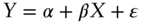 will produce a regression residual,
  , that has the following property:
  . So, if we regress our signal onto sets of indicator variables that capture the various groupings (rating, industry, domicile, etc.) the residual will be orthogonal to those groupings. Demeaning is equivalent when you are looking to remove the influence of one group, but regression is more efficient when dealing with multiple groupings.
 - Beta neutrality: A key criticism of active risk taking by incumbent fixed income managers (across all fixed income categories), as discussed in Chapter 4, was the passive exposure to traditional market risk premia, especially credit markets. We do not want to be guilty of repackaging beta as alpha. We can use the same technique we used for group neutrality. We can regress our signal onto beta (which, of course, requires a measure of beta for every bond in your eligible investment universe), and the residual from that regression is your signal with any beta effect removed. Unlike a grouping, demeaning does not work for beta neutralizing. An added benefit of regression is that you could also remove beta across your groupings as well. As students work through examples, they appreciate how quickly you can lose degrees of freedom here. Choices will need to be made on the granularity of groupings, and typically you will be disappointed (i.e., you will have some ability to neutralize to rating, sector, country, and so forth, but not for fine categories especially when there are multiple dimensions you are trying to neutralize to).
Let's try to make this discussion of signal‐specific investment choices concrete using the example of equity momentum as a signal for a corporate bond long/short portfolio. We have a universe of 195 sufficiently liquid five‐year on the run credit‐default swap (CDS) contracts for North American reference entities (spanning both IG and HY markets). For this set of assets, we have a measure of trailing six‐month equity returns as our signal. Let's see what happens to this signal as we transform it along the various dimensions just discussed.
One approach to create a signal out of a raw momentum measure could be to Z‐score the signal across the entire cross‐section (this means subtract the average momentum for all 195 issuers and divide by the standard deviation of momentum across the 195 issuers). Exhibit 8.3 shows what this does to the signal. You preserve the rank ordering across issuers, and the scale is adjusted (it is normalized). But note the negative association with DTS (beta) as better‐performing issuers tend to have lower spreads, and the imbalance in long and short positions across sectors. Are these intended?
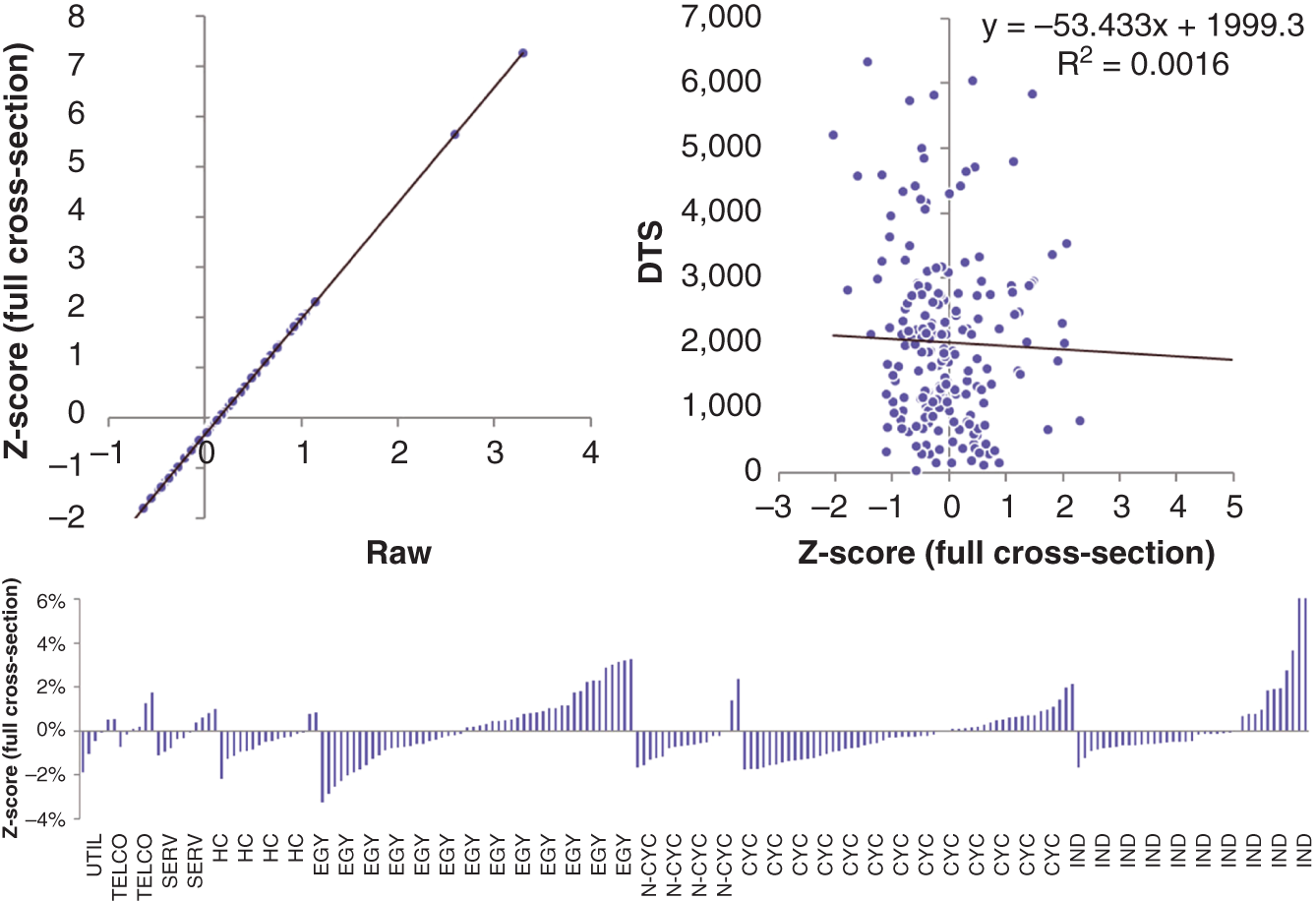
EXHIBIT 8.3 Z‐scored (entire cross‐section) momentum signal for a liquid corporate universe.
An alternative treatment for the momentum measure would be to Z‐score (ranked values) at the sector level rather than across the entire cross‐section. This would ensure there is no sector imbalance across the long and short side of the portfolio. And that is exactly what you see in Exhibit 8.4. There is a perfect balance in negative and positive bars in the sector chart, but there is still a negative tilt to DTS. Even after these adjustments, the modified momentum signal still retains the bulk of the information content of the raw momentum signal (correlation of 0.77).
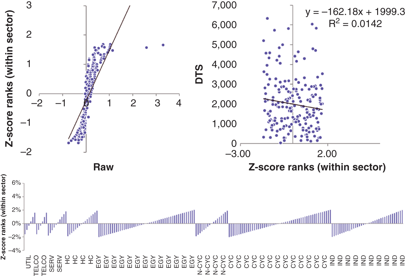
EXHIBIT 8.4 Z‐scored ranks (within sector) momentum signal for a liquid corporate universe.
To remove the negative beta tilt, we can regress the Z‐score within sector momentum measure onto DTS (proxy for beta). Exhibit 8.5 shows how this removes the beta tilt completely but now introduces a small sector imbalance. The solution would then be to regress the Z‐scored within sector momentum measure on a set of indicator variables for sector membership and DTS. A useful exercise for students.
8.3 CHOICES IN THE PORTFOLIO CONSTRUCTION PROCESS (OPTIMIZATION, REBALANCING, TRADING)
Everything in this section speaks to the backward dimension of the investment cube in Exhibit 8.2. Academic research is largely ignorant of this dimension. A simple correlation of a characteristic with future excess return is not a sufficient statistic for success. Let's discuss the many related aspects of portfolio construction that we need to master.
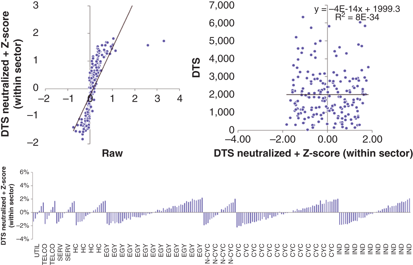
EXHIBIT 8.5 Beta‐neutralized Z‐scored ranks (within sector) momentum signal for a liquid corporate universe.
8.3.1 Objective Function
At the core of any systematic investment process is an objective function. This will typically be seeking to maximize (net of transaction cost) returns while targeting a given level of risk (tracking error) and satisfying various intuitive constraints. An example objective function for corporate bond security selection was introduced in Israel, Palhares, and Richardson (2018), which I reproduce here with some simplifications:

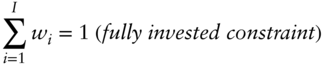

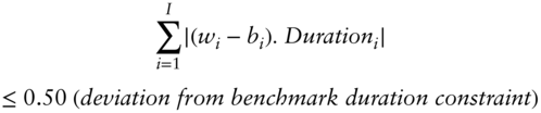
This linear program captures the essential features for our purpose. It is not a mean‐variance optimization. There is no formal modeling of risk via a common factor model (more on that later). But it summarizes what the systematic process is doing. First, the program is solving for a vector of portfolio weights, ![]() . Those weights need to sum to one and all be positive (in the case of a long‐only portfolio). For long‐short portfolios, those constraints would be different. Second, risk is handled here via three separate constraints: (i) deviations from benchmark weights are capped at 0.25 percent (forced diversification), (ii) deviations from benchmark weights are capped in spread units (50 basis points), and (iii) deviations from benchmark weights are capped in spread duration units (0.5 years). Third, the portfolio wants to hold bonds with the highest expected returns,
. Those weights need to sum to one and all be positive (in the case of a long‐only portfolio). For long‐short portfolios, those constraints would be different. Second, risk is handled here via three separate constraints: (i) deviations from benchmark weights are capped at 0.25 percent (forced diversification), (ii) deviations from benchmark weights are capped in spread units (50 basis points), and (iii) deviations from benchmark weights are capped in spread duration units (0.5 years). Third, the portfolio wants to hold bonds with the highest expected returns, ![]() . Additional constraints could be added to limit active risk across various groupings (e.g., sector, rating, country of domicile etc.) and incorporate awareness of liquidity (e.g., portfolio weights may be restricted to be no more than a certain multiple of typical daily trading volumes). This is all very intuitive.
. Additional constraints could be added to limit active risk across various groupings (e.g., sector, rating, country of domicile etc.) and incorporate awareness of liquidity (e.g., portfolio weights may be restricted to be no more than a certain multiple of typical daily trading volumes). This is all very intuitive.
How does a portfolio look once inputs are fed into the objective function? Let's continue with our example of momentum for the corporate universe. We can solve for a set of portfolio weights that maximizes exposure to the beta‐neutralized Z‐scored within sector version of momentum (i.e., ![]() ) while also requiring all portfolio weights to be positive, no weight to exceed 5 percent of the overall portfolio, portfolio weights cannot exceed four times average daily trading volume, and the portfolio must be fully invested. Exhibit 8.6 shows a scatter plot of the optimized portfolio weights against the beta‐neutralized Z‐scored ranks (within sector) momentum signal.
) while also requiring all portfolio weights to be positive, no weight to exceed 5 percent of the overall portfolio, portfolio weights cannot exceed four times average daily trading volume, and the portfolio must be fully invested. Exhibit 8.6 shows a scatter plot of the optimized portfolio weights against the beta‐neutralized Z‐scored ranks (within sector) momentum signal.
At first glance this correlation looks low (it is 0.60) and students initially are uncomfortable. This is not surprising. Your ability to take large positions is limited by liquidity in this optimization setup. If you used additional constraints (e.g., instead of only a 5 percent market capitalization weight limit, also require a risk weight limit) you would see further distance between portfolio weights and your signal. This is the challenge of systematic investing; you want that correlation (called a transfer coefficient as per Grinold and Kahn 2000) to be 1. In the real world, a variety of frictions impede your ability to do so. What can the systematic investor do? Reduce the frictions by preselecting an eligible investment universe that is neither too costly to trade nor too difficult to source liquidity, and improve trading execution. A benefit of visual tools like Exhibit 8.6 is the ability to look at each individual position and understand which constraint is binding, and this can help focus research effort to improve the process (e.g., Do we need better liquidity data to avoid chasing after illiquid bonds? Do we need to enhance modeling of risk to avoid chasing after bonds that have too large a contribution to active risk?)
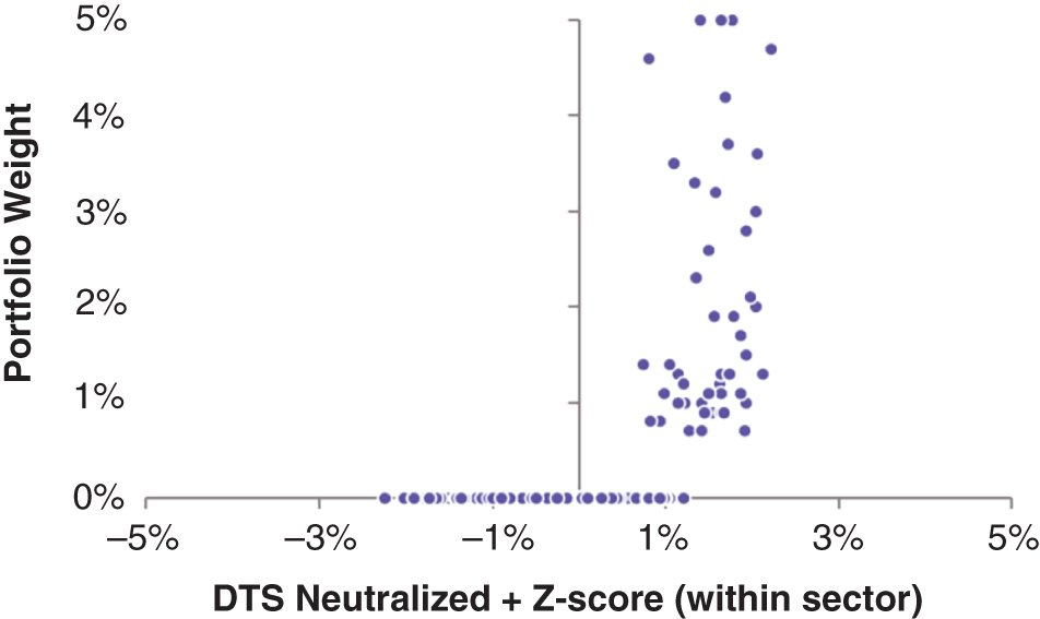
EXHIBIT 8.6 Scatter plot of optimized portfolio weights and the beta‐neutralized Z‐scored ranks (within sector) momentum signal for a liquid corporate universe.
8.3.2 Getting the Units Correct
The objective function does not specify units. The researcher needs to do this. This is important. In our linear program we are trying to maximize expected returns, ![]() . But we are using a combination of transformed signals to generate an aggregate score for each bond. Who knows what unit that aggregate score is expressed in. Grinold and Kahn (2000) introduced the equation
. But we are using a combination of transformed signals to generate an aggregate score for each bond. Who knows what unit that aggregate score is expressed in. Grinold and Kahn (2000) introduced the equation ![]() , which allows for Z‐scored signals to be converted to an expected return by multiplying with your skill (
, which allows for Z‐scored signals to be converted to an expected return by multiplying with your skill (![]() , information coefficient) and the volatility of the asset (
, information coefficient) and the volatility of the asset (![]() ). This presupposes that your signal is in risk‐adjusted units. It may not be. Consider carry, which is already in expected return units. Some thought is needed to map individual signals into return space. An alternative approach is to empirically calibrate how your combination of signals predicts future excess returns (on average). This reduced form approach will get your signal collection into the correct unit. Why is this important? Other constraints in the objective function (e.g., expected transaction costs) will be in return units, so you want the constraints to behave as expected when trade‐offs are made.
). This presupposes that your signal is in risk‐adjusted units. It may not be. Consider carry, which is already in expected return units. Some thought is needed to map individual signals into return space. An alternative approach is to empirically calibrate how your combination of signals predicts future excess returns (on average). This reduced form approach will get your signal collection into the correct unit. Why is this important? Other constraints in the objective function (e.g., expected transaction costs) will be in return units, so you want the constraints to behave as expected when trade‐offs are made.
8.3.3 Modeling Risk
Risk modeling is a topic worthy of its own book. All I want to introduce here are some of the different types of risk models I have seen used by systematic fixed income investors. By risk model I mean the identification of the volatility and correlation structure across the set of assets in your eligible investment universe. If you have 2,000 bonds in your universe, then we are talking about 2,000 measures of volatility and many, many more correlations! These types of risk models are central to the systematic investment process, as they allow investors to target a level of risk in their portfolios, and constraints can also be specified for specific bonds or combinations of bonds to limit active risk (e.g., groupings on sector, rating, etc.).
While there are advocates of purely statistical models of risk that extract information from the time series of returns using the principal components approach, which we covered in Chapter 5, I find them less useful because they are difficult to interpret. Instead, the most common type of risk models will generate ![]() covariance matrices, where
covariance matrices, where ![]() is the number of assets in your eligible investment universe. The elements of the matrix can be identified using (i) asset‐ level historical returns (commonly used for small cross‐sections like government bond portfolios), and (ii) common factor historical returns (commonly used for large cross‐sections like corporate bonds).
is the number of assets in your eligible investment universe. The elements of the matrix can be identified using (i) asset‐ level historical returns (commonly used for small cross‐sections like government bond portfolios), and (ii) common factor historical returns (commonly used for large cross‐sections like corporate bonds).
Armed with a risk model, it is possible to move backward and forward between a portfolio and the expected returns that are implied by that set of portfolio weights. A regular mean‐variance objective function maximizes the following: ![]() , where the first expression,
, where the first expression, ![]() , is the portfolio level expected return and the second expression,
, is the portfolio level expected return and the second expression, ![]() , is portfolio level risk (
, is portfolio level risk (![]() is the covariance matrix for the returns of the assets in the portfolio), with an aversion parameter,
is the covariance matrix for the returns of the assets in the portfolio), with an aversion parameter, ![]() . This function is written in matrix form, so the superscript T refers to transpose. The general solution to this type of objective function is:
. This function is written in matrix form, so the superscript T refers to transpose. The general solution to this type of objective function is: ![]() . Your collection of signals can represent a desired set of portfolio weights,
. Your collection of signals can represent a desired set of portfolio weights, ![]() , and, using this solution, those portfolio weights imply a set of expected returns,
, and, using this solution, those portfolio weights imply a set of expected returns, ![]() . Risk models are versatile tools that are useful not only in optimizations but also in constructing your return forecasts.
. Risk models are versatile tools that are useful not only in optimizations but also in constructing your return forecasts.
There are many choices involved in the modeling of risk, including: (i) look‐back periods for the estimation of return volatility and correlation structure (shorter for volatility and longer for correlations), (ii) inclusion of economic priors on the magnitude of volatilities and correlations (various types of shrinkage estimators can be used, with shrinkage to a peer group average quite common), (iii) separately modeling common factor and idiosyncratic return volatility, and (iv) selection of common factors to include in a cross‐sectional risk model (e.g., which industry classification schema; consistency of investment signals used in your return forecast; and your risk forecast, liquidity, rating, etc.). Estimating your own risk model has the enormous benefit of transparency and flexibility. You know the structure you have imposed to estimate volatilities and correlations. If you want to modify something, it is easy to do so. The downside is the effort to develop and maintain the risk model infrastructure. Commercial third‐party data providers exist for fixed income risk models including BARRA, Axioma, and Northfield.
8.3.4 Rebalancing (Turnover Budget)
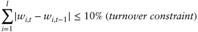
A systematic investment process is run in discrete time. That means you look to rebalance your portfolios at periodic intervals. Traditionally, systematic benchmark‐aware, long‐only portfolios were rebalanced at approximately a monthly frequency. With the advent of liquidity provision strategies, rebalancing is now more frequent and spread over the month. A rebalance is trigged by (i) flows (i.e., redemptions or subscriptions to the fund), (ii) cash flow accumulation (i.e., receipt of coupons from bonds or early receipt of principal due to tenders, calls, and other corporate actions), and (iii) drift in your portfolio from the optimal portfolio. The first two types of rebalance triggers are easy to track (simply look at the amount of uninvested cash in your portfolio and when that gets too large you rebalance). The third type of trigger is an ongoing assessment. We mentioned the term “transfer coefficient” (TC) earlier in this chapter. In a rebalancing context, the TC is a (risk‐weighted) measure of distance between the portfolio you hold and the portfolio that you would like to hold (the optimal portfolio). As that distance grows, the utility from rebalancing increases. Portfolio managers watch measures of TC to decide when to rebalance. Of course, rebalances should also be timed to correspond to normal periods of liquidity (i.e., don't rebalance a portfolio on Wednesday prior to Thanksgiving holiday, and don't rebalance a rate‐sensitive asset portfolio the morning of a Federal Open Market Committee meeting).
What is the optimal amount of turnover? This is a difficult question to answer, because it is highly endogenous. Your combination of signals will have a natural horizon over which returns are forecasted (typically higher returns in the short horizon and lower returns in the longer horizon). All else equal, the faster your signal (i.e., the quicker the speed of decay of your return forecast) the higher the turnover needed for your portfolio. But, how do you determine the speed of your return forecast? By looking at the data (in‐sample or via live experience). The speed of your model should also respect the underlying liquidity of the market. There is a reason that high‐frequency trading is limited to equity markets and liquid futures markets. You need low latency (i.e., the ability to trade within a micro‐second). As we will see in Chapter 9, corporate bond markets do not have anything close to that type of latency. Furthermore, as noted in Israel, Palhares, and Richardson (2018), expected trading costs for corporate bonds are high relative to the underlying volatility of the asset class (see also Harris 2015). This means that turnover needs to be carefully assessed against the expected transaction costs (the positive utility from increased expected returns needs to be traded off against the negative utility from increased costs paid to trade toward the optimal portfolio). This is where improvements to order management and trade execution systems can have a large impact on the portfolio: they allow you to trade more aggressively toward the optimal portfolio and increase the TC.
8.3.5 Constraints
There are various other constraints that could be incorporated into a systematic investment process, and I discuss them briefly here.
- Beta constraints: Typically, a long‐only benchmark‐aware portfolio targets beta = 1 and an unconstrained long/short portfolio targets beta = 0. Other beta levels could also be targeted. Whatever the target, a portfolio level constraint can be incorporated (e.g.,
 ) that ensures your portfolio weights match the beta of the benchmark. Note that this type of constraint can also be expressed in active weight space (i.e.,
  ). Beta constraints can operate at the portfolio level or could also operate at a subgroup level within the portfolio (e.g., you may want to limit the active risk taken across rating categories or across industry groups).
 - Trade‐size constraints: Unlike equity markets most fixed income securities do not trade on electronic exchanges where orders can be broken up into small pieces (e.g., 100 shares). Instead, there are socially acceptable regular trade sizes. Although these have trended down over time as electronification of the markets has increased (more on this in the next chapter), there is still a need to trade at minimum sizes. This type of constraint is nonlinear and can cause challenges for efficient solutions, but it is a topic that needs to be addressed.
- Position size constraints: The optimal portfolio weights should also be a function of the underlying liquidity of the market, so the weight for a given bond will typically be capped at a multiple of expected trading volumes. Risk officers also carefully look at portfolio level statistics based on these measures: How many days would it take to liquidate the portfolio in regular market conditions? Capacity considerations are directly related to this type of constraint. The tighter you make this constraint (perhaps because the investment vehicle allows for daily dealing), then the smaller the positions you can build in any one bond. Combined with other constraints (especially issuer weight limits) this naturally caps the size of the portfolio you can manage.
- Sustainability: This is a multifaceted term that can mean many different things and asset owners are increasingly paying attention to aspects of sustainability (ESG). We have an entire chapter dedicated to this topic. For now, note that constraints are often an efficient way to incorporate sustainability considerations into a portfolio with the objective of not sacrificing risk‐adjusted returns. This is where systematic investment processes are strictly superior to traditional discretionary approaches. When you have multiple objectives for a portfolio, it quickly becomes very difficult to keep track of the correct trade‐offs.
- Other constraints: Systematic investment processes evolve over time, and without fail you will learn things along the way. Beware the knee‐jerk reaction of blindly adding constraints to the portfolio in response to an unintended exposure that generated a negative return realization. Yes, you do want to mitigate tracking error coming from sources that are not well compensated, but such constraints do not come for free, they lower your TC. You need to be convinced that every constraint is necessary for your portfolio, otherwise as time passes you will be adding more constraints, and be solving for those constraints, and drifting away from your primary objective: chasing bonds with the highest expected returns. As Richard Grinold used to say, beware the “whack a mole”!
8.3.6 Mixing or Integrating Signals
Our analysis of portfolio construction has worked with one portfolio. It is formed based on integrating across all investment insights. This has the benefit of utilizing information across return forecasting sources, especially the correlation structure across investment signals. An alternative approach would be to invest capital (or risk) across separate portfolios that targeted each investment theme separately. This has the benefit of very clean attribution: you can see the performance of each theme very clearly. However, it suffers from a distinct drawback insofar as you will be buying and selling securities across these portfolios due to canceling views (i.e., you may like a bond in a value portfolio but dislike the same bond in a momentum portfolio). In asset classes, where trading costs are high, such as corporate bonds, mixing across separate portfolios seems to be inefficient. For a full examination of this topic in the context of equity markets see Fitzgibbons, Friedman, Pomorski, and Serban (2017).
8.4 OTHER TOPICS
8.4.1 Crowding
Any discussion of systematic investing seems to be incomplete without talking about “crowding.” Why this fear seems to be unique to systematic investors is a bit of a mystery. Anyhow, the concern seems to be that as more people know about the investment thesis, the worse it will be. Although that sounds compelling, there are multiple issues with this. Asness (2016) provides an excellent discussion and summary of the key issues. I will just restate a couple of elements of that paper. First, simple knowledge of an investment thesis is insufficient to erode its return potential. Capital needs to be invested to erode that expected return edge. Second, while the capital is invested, to chase the investment thesis the return experience would be very positive (flow induced). But going forward, returns may be lower. Third, capital chasing an idea may not remove its return potential if the basis for the return relation is linked to nondiversifiable risk (as opposed to cognitive errors by capital market participants). Fourth, the presence of levered investors coupled with the risk of crowding introduces an element of deleveraging risk (see also Richardson, Saffi, and Sigurdsson 2017).
As Asness (2016) neatly summarized, a rational forecast of the risk of crowding, at least directionally, is a reduction in expected returns and an increase in risk. The combined effect is a lowering of risk‐adjusted returns, not to zero, but a lowering. But does this type of risk apply to systematic fixed income investing? Not yet. Wigglesworth and Fletcher (2021) note that estimates of the quantitative strategies in fixed income are tiny relative to the size of the fixed income markets and quantitative fixed income strategies account for about 3 percent of the assets invested in quantitative equity strategies. So, while crowding is a risk to monitor, it does not seem to be top of the list now.
8.4.2 Beta Completion
My final discussion point on portfolio construction speaks to beta completion. Chapter 4 had noted a systemic shortcoming of beta repackaged as alpha for many active fixed income managers. To avoid that criticism in our systematic approach, we need to be sure that our active risk is not driven by beta views. At the same time, for long‐only benchmark‐aware portfolios, we need to be sure to give the asset owner the beta embedded in their benchmark. For fixed income investments, that is a multidimensional challenge. All fixed income assets inherit exposure to the local currency‐yield curve (risk‐free component), all credit‐sensitive assets have additional exposure to the local credit curve (risky component), and for global mandates there are multiple currencies reflected in the benchmark.
Our systematic investment process is designed to solve for a set of portfolio weights consistent with the objective function (inclusive of constraints). That portfolio also needs to match the risk‐free, risky, and currency exposure of the benchmark. This can be achieved via additional constraints that limit active risk across those dimensions. Or, and what I would strongly recommend, is to use derivatives to complete the beta of the portfolio, especially for credit‐sensitive assets that are expensive to trade individually. Why would you want to distort your optimal portfolio to balance interest rate risk, currency risk, or credit risk? There are much cheaper instruments to adjust positioning along these dimensions (e.g., interest rate derivatives, typically swaps and futures, to manage rate risk; credit index derivatives to manage overall credit risk; and currency forwards to manage currency risk). Of course, this means that investment guidelines need to be structured to allow the use of these derivatives. The process of beta completion across these dimensions requires estimation of (i) the beta contribution of each asset to rate and credit risk, and (ii) the sensitivity of your elected derivative to the beta you are completing. Again, more choice and estimation is needed, but these are essential ingredients for a successful systematic investment process.
REFERENCES
- Asness, C. (2016). How can a strategy still work if everyone knows about itt? AQR working paper.
- Fitzgibbons, S., J. Friedman, L. Pomorski, and L. Serban. (2017). Journal of Investing, 26, 153–164.
- Grinold, R., and R. Kahn. (2000). Active Portfolio Management. McGraw‐Hill.
- Gupta, T., and B. Kelly. (2019). Factor momentum everywhere. Journal of Portfolio Management, 45, 13–36.
- Harris, L. (2015). Transaction costs, trade throughs, and riskless principal trading in corporate bond markets. University of Southern California, working paper.
- Israel, R., D. Palhares, and S. Richardson. (2018). Common factors in corporate bond returns. Journal of Investment Management, 16, 17–46.
- Richardson, S., P. Saffi, and K. Sigurdsson. (2017). Deleveraging risk. Journal of Financial and Quantitative Analysis, 52, 2491–2522.
- Wigglesworth, R., and L. Fletcher. (2021). The next quant revolution: Shaking up the corporate bond market. Financial Times (December 7).