
Chapter six. Operational Thinking
Dynamic Systems: Dealing with Chaos and Complexity
Relationships are all there is to reality.
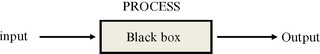
Relationships are all there is to the reality and operational thinking is about mapping these relationships. It is about capturing interactions, interconnections, and the sequence and flow of activities. It is about how systems do what they do, the dynamic process of producing emergent properties — life, love, happiness, success, throughputs — online and real-time. In a nutshell, it is about unlocking the black box that lies between system inputs and its outputs. To think about any thing requires a mental image or model of it. A mental model is a selective abstraction of reality and at best it is an oversimplification. However, we do experience extreme difficulty when creating a working mental model of even a simple dynamic phenomenon or attempt to visualize the behavior of interdependent variables. It seems that our cognitive abilities have mostly developed to deal with the static models concerning “here” and “now.” Operational thinking is an ingenious way to overcome the difficulties encountered in constructing and simulating complex, dynamic mental models.
Keywords: Air traffic; Closed loop thinking; Complexity; Counterintuitive; Delayed response; Deregulation; Derivatives; Emergent property; Exponential growth; Carrying capacity; Financial crisis; Hedge funds; Housing bubble; Interactive model; Interdependency; Invisible hand; i-Think model; Linear; Mental image; Nonlinear; Open loop thinking; Pattern recognition; Purposeful system; Re-engineering; Resonance; Rhythm; Securitization of mortgage; Selective abstraction; Synergy
Operational thinking is about mapping relationships. It is about capturing interactions, interconnections, the sequence and flow of activities, and the rules of the game. It is about how systems do what they do, or the dynamic process of using elements of the structure to produce the desired functions. In a nutshell, it is about unlocking the black box that lies between system input and system output.
There are certain things about the behavior of complex systems that are more related to the way they are organized than the characteristics of their individual parts. We call them emergent properties, for they are the property of the whole not the parts. Examples include love, life, success, and development. In a different context self-maintaining, goal-seeking, self-organizing, and purposeful systems also represent another form of emergent behavior.
An emergent property is the end result of a dynamic process that operates online and in real time. When a living system dies it loses this “livingness property”; the self-organizing behavior that held it together no longer functions.
Furthermore, the social dynamic represents a level of complexity that is beyond the reach of conventional thinking. The late Barry Richmond, creator of the iThink1 model, believed “the way we think is outdated. As a result, the way we act creates problems, and we are ill-equipped to address them because of the way we think” (Richmond, 2001).
Apparently our highly regarded conventional tools are not doing their jobs. Otherwise how could we explain the sorry fact that we have been applying the same set of non-solutions to crucial social problems such as drugs, poverty, crime, illiteracy, and maldistribution of wealth for most of the last 50 years, with no obvious sign of any new learning? Why do so many well-intended performance improvement efforts, conceived by so many smart people, so often miss the mark? Most re-engineering efforts have failed, major projects have overrun by very large margins, and the mergers and acquisitions have not been able to realize anticipated synergy. Let us examine Richmond's assertion about thinking a little further.
To think about anything requires a mental image or model of it. A mental model is a selective abstraction of reality and at best it is an oversimplification. In addition, our cognitive abilities have unfortunately developed to deal with the static models concerning “here” and “now.” It has evolved around assumptions of unidirectional causality or open loop thinking. Therefore, we experience extreme difficulty when creating a working mental model of even a simple dynamic phenomenon or attempt to visualize the behavior of interdependent variables.
To capture the multidirectional interactions of interdependent variables and to map a dynamic process, we first need to use a pictorial language. As observed so elegantly by Donella Meadows (2008):
Words and sentences must, by necessity, come only one at a time in a linear, logical order. Systems happen all at once. Their elements are connected not just in one direction, but also in many directions simultaneously. Pictures work for this language better than words, because you can see all the parts of a picture at once.
Therefore, in mapping the dynamic processes, we will rely more heavily on pictorial presentation rather than the written language. We also need to have a better understanding of the source and nature of complexity. Finally, we need an operational modeling tool that can explicitly display the interdependencies, the underlying assumptions, and the richness of the dynamic phenomenon under study.
6.1. Complexity
Complexity is a relative term. It depends on the number and the nature of interactions among the variables involved. Open loop systems with linear, independent variables are considered simpler than interdependent variables forming nonlinear closed loops with a delayed response. Key words in the above statement are open loop, closed loop, linear, nonlinear, and delayed response.
6.1.1. Open Loop and Closed Loop Systems
The first step in understanding complexity is to appreciate the iterative and thus dynamic nature of closed loop systems and their counterintuitive behavior. Consider the following two simple examples:
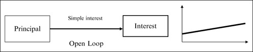
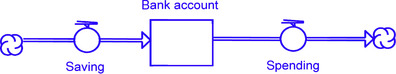
1. A savings account in a bank earning a simple 10% interest reflects an open loop behavior. Both yearly earnings and the amount of principal ($10,000) remain constant and the total sum (principal plus interest) would increase at a slow pace (see Figure 6.2). After 56 years, $66,000 would accumulate in this account.
2. However, if the savings account was to earn 10% compound interest, it would represent a closed loop behavior and the money in the savings account would grow exponentially, doubling every seven years. The initial principal of $10,000 would grow to $1,280,000 in 56 years (see Figure 6.3).
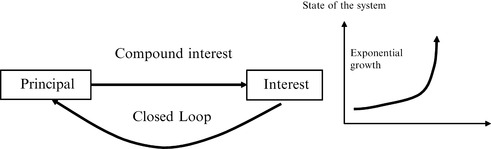
Now compare this amount with the $66,000 that would have been earned with the simple interest example to better understand the dramatic difference in behavior.
6.1.2. Linear and Nonlinear Systems
If the interest rate in the previous example varied according to market conditions then we would be facing a nonlinear system. In closed loop thinking, linear and nonlinear refer to the rate of change, not the state of a system (see Figure 6.4).
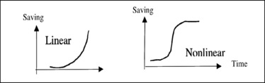
Please note that most of our mathematical tools are based on the assumption of linearity rather than nonlinearity. In a linear system, a value for the whole can be reached by adding the value of its parts (type I property). Nonlinearity, by contrast, is characteristic of an emergent property where the whole is the product of interactions of the parts.
With his pioneering work on dynamic behavior of systems, J.W. Forrester (1971) observed that reinforcing (positive) and counteracting (negative) feedback loops are responsible for creating counterintuitive behavior.
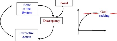
Let us first look at the dynamic behavior of a simple negative feedback loop (which we will call goal-seeking). A thermostat best describes it. Room temperature is set to a desired degree (goal). Periodically discrepancies between the current state of the system (room temperature) and the goal are measured and used to initiate corrective actions to bring the state of the system closer to the goal (see Figure 6.5).
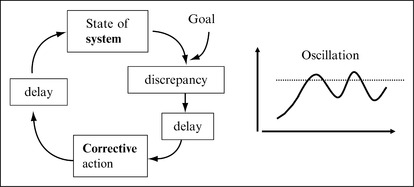
6.1.2.1. Effects of a delayed response
Introducing a delay function to our simple negative feedback loop will produce an unexpected oscillation (a counterintuitive behavior). For example, a delay between the time a discrepancy is observed and a corrective action is taken will result in an oscillation in room temperature (see Figure 6.6).
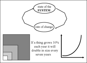
Second, we will consider the common phenomenon known as a positive feedback loop, such as a bank account earning compound interest or a company growing annually at a fixed rate. We said that it would result in an exponential growth curve (see Figure 6.7).
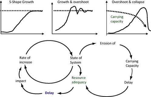
The exponential growth curve resulting from a positive feedback loop assumes unlimited resources, but in reality, a resource is a universal constraint and all exponential growth curves will eventually be influenced by carrying capacity and therefore will ultimately convert to an S-shaped curve.
6.1.2.2. Impact of carrying capacity
Now, if we just add the impact of carrying capacity to our simple positive feedback loop, we will create a counteracting double loop system producing an S-shaped curve. Superimposing a delay function, another unavoidable reality, will produce the same type of oscillation we experienced in the previous example. The overshoot and collapse scenario reflects the cases where the growth strategy has an additional negative impact on the carrying capacity of the system. This phenomenon explains the collapse of dotcoms, the fiasco of Enron, the housing bubble, and the faith of thousands of corporations that pursue a blind long-term growth strategy with no regard for the limitations imposed by the carrying capacity of the system and/or its environment (see Figure 6.8).
6.1.2.3. Understanding the multi-loop nonlinear feedback system
Please note that by combining a few simple and ordinary phenomena we have managed to create a multi-loop nonlinear feedback system. This is the infamous monster that, according to chaos theory, produces chaotic behavior. Unfortunately, as you can see, the monster is not an unusual phenomenon and it is much more common than we have been led to believe. The point to emphasize is that the interaction of counteracting feedback loops — the prime source for generating chaos and complexity — is a common phenomenon in our daily lives. Understanding these dynamics is the key to getting a handle on the notions of complexity, interdependency, and counterintuitive behavior of social systems. For an in-depth discussion of dynamic behaviors of feedback loops see Business Dynamics (Sterman, 2000). Furthermore, and in a different context, Stephen Wolfram (2002), in New Kind of Science, makes an important observation:
The idea of describing behavior in terms of mathematical equations works well where the behavior is fairly simple. It almost inevitably fails whenever the behavior is more complex. Indeed, there are many common phenomena about which theoretical science has had remarkably very little to say. Degree of difficulty encountered in mathematical representation of a phenomenon increases exponentially by the degree of its complexity.
Wolfram then goes on to demonstrate how systems too complex for traditional mathematics could yet obey simple operational rules. With his now famous cellular automata, Wolfram demonstrated how iteration of remarkably simple rules could produce highly complex systems. By developing a computer program, he was able to reproduce the essential characteristics of complex phenomena. His “new kind of science” makes it possible to capture the operation of a self-organizing system and understand how disordered systems spontaneously organize themselves to produce vastly complex structures.
Operational thinking is an ingenious way to overcome the difficulties encountered in constructing and simulating complex mental models. Relying solely on mathematical representation for dealing with complex phenomena has been a practical nightmare. Operational modeling and use of programs such as iThink software have made it practical to get a handle on the increasingly relevant complex phenomena.
Although multi-loop nonlinear feedback systems exhibit chaotic behavior, there is an order in this chaos. Such systems seem to produce particular patterns of behavior.
Discovering the pattern of behavior for our system of interest is the key for recognizing the hidden order that is locking the system into its present course. Unless the hidden orders are made explicit and dismantled, the current behavior will outlive any temporary effects of interventions no matter how well intended.
In this context recognizing the rhythm or the iterative cycle of a closed loop system is the first step toward understanding the dynamics of change and emergence of organized complexities.
Remember that to map the dynamic behavior of a system is to capture the interaction of positive and negative feedback loops. These interactions, in essence, define the interdependencies, which in turn are responsible for nonlinearity in the system. It is the interdependency that poses the major challenge to our cognitive abilities. It is this challenge that we need to overcome by using operational modeling. Pattern recognition is critical for understanding and changing undesirable behavior. This leads us to the need for development of interactive operational representation of the phenomenon under investigation.
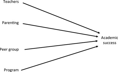
Let us consider factors that we assume contribute to academic success. A conventional approach normally uses a laundry list approach by assuming that the success factors — good teaching, good parenting, good peer group, and a good programming — each act independently, contributing directly to our academic success (see Figure 6.9).
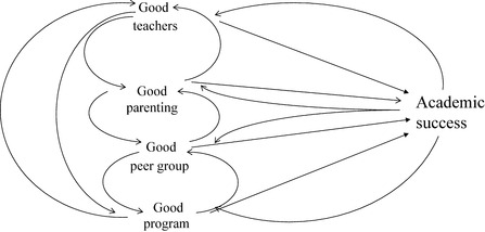
However, good teaching, good parenting, good peer-grouping, and good programming are not the only things that contribute to academic success. We do know that academic success creates an environment to attract good teachers, good parents, and good peer groups as well as reinforces good programming. In addition we may also agree that good parenting reinforces good teaching and good peer-grouping, and in the similar way good teaching reinforces good programming and good parenting and so forth. Therefore, Figure 6.10 is a more realistic representation of this dynamic case. It captures interdependencies and the closed loop nature of the relationships and highlights the possibility of emerging synergy and resonance among the variables.
The following is an “interactive model” of the current financial crisis. It re-emphasizes the old truth that the road to the hell is paved with good intentions. A bipartisan coalition to expand home ownership to the lower middle class and the poor created two reinforcing feedback loops that resulted in the housing bubble and subsequent financial crisis of 2008. The first loop was created by securitization of subprime mortgages. The illusion that mortgages are insured by institutions backed by the U.S. government — Fannie Mae and Freddie Mac — relieved the mortgage providers from any responsibility or liability for the riskiness of the loans they issued. The shady loans were immediately re-sold in the multi-trillion-dollar security markets. Investment bankers with their risk-free, volume-based business models played the insatiable demand for the dubious securities to the end. The Federal Reserve's low interest rate policy (the second loop) further reinforced this game by fueling a fictitious housing market. Suppose you can afford to pay $1,000 for a monthly mortgage. With a 10% rate of interest you will be in the market for a house priced around $100,000. If the interest rate drops to 5%, with the same $1,000 you can afford a house around $200,000. With an interest rate of 2.5%, you can look for a house price around $400,000. Now if the variable rate drops to 1.25% and mortgage providers are willing to loan you enough money with no concern about your financial situation, you will go for the house priced around $800,000. The game goes on until the fictitious housing bubble collapses (see Figure 6.11).

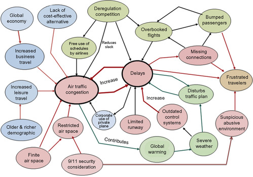
Those who travel to earn a living will not be able to hide their frustration about the state of air travel. Deregulation of the airlines, free use of air space, and autonomy of the airlines to schedule their flights, combined with the lack of any cost-effective alternative means to travel have resulted in a mess that is not going to be dissolved easily. Most of the airports in the Eastern corridor are operating at 20% above their normal capacity. Therefore, delays and canceled flights are as normal as small variations in the weather. The system that has used up all of its buffers is vulnerable to even the smallest of deviations. Post-9/11 security considerations increased air-space restrictions in the Eastern corridor. This, combined with the outdated air traffic control systems and the increased use of small private planes (a small plane with a few passengers takes the same air bubble required by a Boeing 747 with 500 passengers on landing and takeoff) contribute heavily to the air traffic congestion. Adding the demands of the global economy as well as travel demands of the ever-increasing richer and older generations to already overloaded air traffic aggregate the unpleasant mess illustrated in Figure 6.12.
To summarize, appreciation of the following principles is the key for getting in tune with operational thinking:
• It is easier to predict the behavior of the parts by understanding the behavior of the whole than to predict the behavior of the whole by understanding the behavior of the parts.
• True understanding of operational thinking comes with the realization that time is not really defined by an arrow but by the “beat,” or the rhythm and appreciation of the iterative nature of complex phenomenon.
• Getting the beat — periodic repeats of a predefined set of operations — is essential to getting a handle on the closed loop systems and discovering the hidden order responsible for regenerating chaotic patterns of behavior.
• To think one needs to use a mental model, but mental models are only an abstraction of reality and at best an oversimplification. Making them explicit is the only chance one has to learn and improve them.
• One cannot control a complex social system, but can redesign or dance with it. To get a handle on a complex system (Meadows, 2008):
Watch how it behaves
Learn its history
Direct your thought to dynamic, not static analysis
Not only to “What is wrong?” but “How did we get there?”
Search for the why question, why system behaves the way it does.
6.2. Operational thinking, the ithink language
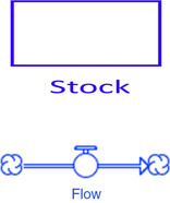
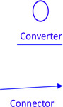
There are four basic icons in the language of operational thinking: stock, flow, converter, and connector (see Figure 6.13). These four symbols form a complete set for a context-free universal modeling language capable of capturing the essence and simulating the behavior of complex dynamic social phenomena.

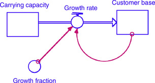
Stock: State of beings, state of a variable, things that accumulate, are measured, or are quantified, for example, customer base, market potential, and cash in bank accounts. Love in your heart, quality of the product, customer satisfaction, demand, supply, workforce, and skill level are also considered stock. It can represent any resource (both type I and II). It can be constraints (carrying capacity), buffer (slack), or inventory that accumulates on store shelves, in transport trucks, and in warehouses. It can also be used to represent conveyors to define transit times and/or delays.
Flow: Represents action over time, the beat (periodic repeats of a predefined set of operations), and the rate of change that is the action (minute, hour, day, month, or year). It is the means to change the state of the variables under consideration (adding or subtracting). It also defines activity, things in motion, earning, spending, getting angry, becoming frustrated, learning, selling, buying, hiring, and firing.
Note that the only way you can change the value of a stock is by an inflow or an outflow (Figure 6.14). But a flow can be influenced by stocks, by other flows, and by converters (Figure 6.15). Flow can also be constrained by a stock (carrying capacity).
Converters, signified by circles, represent constants, conversion tables, equation conditions, graphical relationships, iThink functions, and all of the factors or variables that do not accumulate but have an influence on the behavior of a flow.
6.2.1. Connectors
Connectors, signified by pointers, essentially define the critical feedback loops signifying the relationships and capturing the interdependencies among the variables. They explicitly define what depends on what and what influences what (Figure 6.16).
6.2.2. Modeling Interdependency
iThink operational models are used in a variety of problem situations, but I especially prefer to use them in the following two contexts:
1. To formulate the mess — the future implicit in present operation (see Chapter 8).
2. To investigate the behavior of interdependent variables and capture the dynamic interactions of the phenomenon under study. For this purpose I designate each critical variable with a stock and its corresponding inflow and/or outflow, then use the necessary convertor and connectors to establish their relationship and the defining feedback loops.
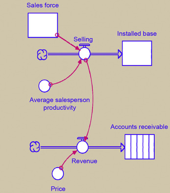
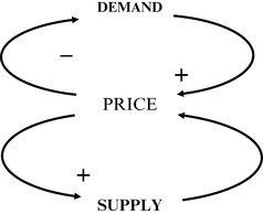
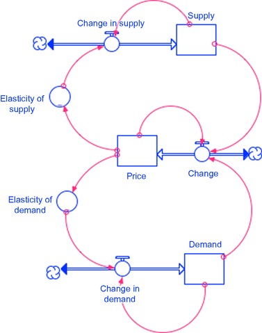
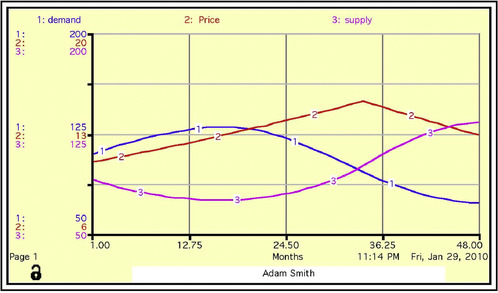
The following model is a simple but beautiful classic example of how an iThink operational model handles the phenomenon of interdependency. Two simple feedback loops capture the essence of Adam Smith's famous “invisible hand,” which, in essence, is about the interactions of three interdependent variables (Figures 6.17 and 6.18). Notice that all three interdependent variables are represented by a stock and corresponding bi-flows that will change them. Price in accordance with the elasticity curve for each supply and demand determines the changes in the supply and demand levels, and price in turn is influenced by the relationship between supply and demand. The formula used calls for a 1% increase in price if demand is greater than supply and a 1% decrease in price if demand is less than supply. Price will not change if supply and demand are equal. The connectors capturing the feedback loops and converters are used to represent the elasticity of the demand and supply curve. Figure 6.19 is the simulated output of the above mentioned iThink model.
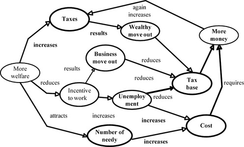
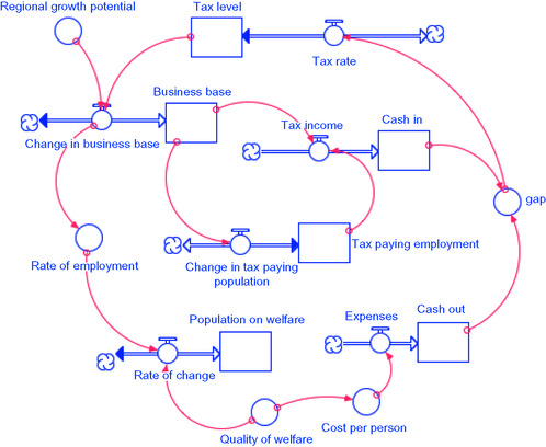
The regional welfare system is an example of how to use the interactive operation model and iThink operation model to formulate the “mess.” It demonstrates how an attractive regional welfare system created on the concern for distribution of wealth could result in two interacting feedback loops that counteractively undermine the original good intention. The increased taxes — to pay for the welfare cost — force both businesses and wealthy people to move out of the region, thus reducing the tax base. With another loop the attractive regional welfare system attracts additional poor people from neighboring regions, therefore increasing the cost of the welfare system. Increased cost combined with reduced revenue, as a result of a reduced tax base, necessitates another round of tax increases, promoting a vicious circle (see Figures 6.20 and 6.21).
6.3. Dynamics of throughput systems
In a global economy, price is set by the global market, making it an uncontrollable variable. This renders Sloane's famous “cost plus” pricing policy obsolete. Sloane's famous assertion, that cost is an uncontrollable variable and price consisting of cost plus a reasonable profit is the controllable variable, led to a dominating cost plus economy in America that lasted for a long time. But the game has changed. Today, the only way to compete is to reduce cost, improve throughput by periodically redesigning the product and throughput processes, and remembering that 75% of the cost is design driven. But to improve throughput requires that we deal with the following four interdependent variables simultaneously: cycle time, cost, flexibility, and quality. This can only be done by building a dynamic model of the throughput process that is capable of dealing with interdependent variables.
We have defined throughput as the process of generating and disseminating wealth. It contains all of the activities necessary to obtain required inputs, convert inputs to outputs, and then take the final products to market. Therefore, marketing, selling, order processing, purchasing, producing, shipping, billing, and accounting — in addition to cash management, quality, time, and cost — are among the activities of a throughput chain.
The list of activities for a service industry might be slightly different; for example, throughput of an education system will include activities for selecting and registering students, scheduling the courses, teaching, giving exams, and issuing certifications. Meanwhile, the throughput of a health-care system may include access to patients, access to health-care providers, interface with third-party payers, delivery of health care, delivery of patient care, and management of the reimbursement system.
Nevertheless, it is obvious that even a simple throughput consists of a chain of events and activities that need to be integrated. Since these activities are usually carried out by different groups in different departments of an organization, strong interface and effective coupling among them are a must for a competitive throughput.
Actually, to design a throughput system, we need to
• Know the state-of-the-art, as well as availability and feasibility of alternative technologies and their relevance to the emerging competitive game
• Understand the flow, the interface between active elements, and how the coupling function works
• Appreciate the dynamics of the system such as the time cycle, buffers, delays, queues, bottlenecks, and feedback loops
• Handle the interdependencies among critical variables, plus deal with open and closed loops, structural imperatives, and system constraints
• Have an operational knowledge of throughput accounting including target costing and variable budgeting
Figure 6.22 describes elements of a holistic approach to designing a throughput. The basic elements of this scheme are the critical properties of the process, model of the process, and the measurement and learning system.
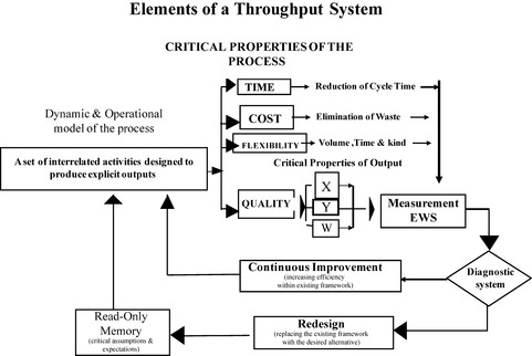
6.3.1. Critical Properties of the Process
The most important element in our throughput scheme is identification of critical properties of the process. Time, cost, flexibility, and quality are usually among the major factors that determine the success of a throughput process. They form an interdependent set of variables so that each one can be improved at the expense of others. Treating them as independent variables, as is normally done, is an unacceptable mistake. Unfortunately, expertise is in any one of the areas of time cycle reduction, cost control or waste reduction, and quality control. Each expert tries to suboptimize the single area of her/his concerns by manipulating the process. This might lead to incompatibility among the solutions. The challenge is to reduce cycle time, while eliminating the waste and ensuring availability of the output (in kind, volume, space, and time), in addition to managing the process in such a way that it is “competent and in control” all at the same time. This can only be done by simulating the throughput process by building a dynamic model.
6.3.2. Model of the Process
The model of a throughput process in its simplest form is a set of interrelated activities designed to produce an explicit output. Different ways and several levels of sophistication can be used to model a process. The most common is a simple flow chart. However, to get a handle on interdependencies and the dynamics of the system, I like to use the iThink software to simulate throughput processes. In addition, I believe Eliyahu Goldratt's (1997) constraint theory or more specifically his book, Critical Chain, is a must read and a fitting complementary tool to our throughput modeling formulation.
In Critical Chain, Goldratt, by recognizing principles of multidimensionality and emergent property, demonstrates beautifully why local optimization does not lead to global optimization. Using the chain as an analogy for a throughput he asserts that the strength of the chain represents the throughput of a process, and the weight of the chain represents its cost. Then he goes on to argue why we have lost the luxury of choosing between increasing the throughput or reducing the cost, why the old dichotomy is not valid anymore, and that to survive we need to increase throughput and reduce cost at the same time.
Since the strength of a chain is defined by its weakest element, he proposes an iterative process of strengthening the weak links in sequence of the weakest link first. Each iteration improves the throughput to the next limit defined by the next weakest element with a minimum cost, thus eliminating the cost of over-designs.
Then using his ingenious observation that time estimated to finish a task with 80% of confidence is three times greater than the most probable time it takes to finish the task (see Figure 6.23) Goldratt develops an elegant scheme that artfully uses buffers to significantly reduce time, minimize waste, and improve flexibility of a throughput process.
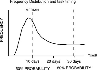
Note that the area under the curve is the probability of finishing the task on time. The higher the uncertainty, the longer the tail of the distribution. Median means that there is only a 50% chance of finishing at or before this time.
To reiterate our early discussions about developing a dynamic model of a throughput process, I would like to re-emphasize the point that the simplest way to build a dynamic model is to identify and map the behavior of the relevant throughput variables, the manner in which the variables change, and the way they relate to one another. Using a simplified version of the conventions and icons provided by the iThink program — stocks, flows, converters, and connectors — we can map the behavior of each variable separately and then put them all together in a web of interde-pendencies.
The following example represents a real case of throughput modeling using iThink. In 1997 I received a request from a prominent telephone company for help to overcome a critical challenge in their throughput system — the inability of the existing structure to serve the rapidly expanding customer demand to meet the requirements of the Internet era. Unprecedented demand had resulted in unacceptable levels of malfunctioning of the throughput system. Consequently, customer complaints had reached such a level that the FCC had been forced to impose crippling financial penalties on the company.
The four interdependent throughput activities — installation, repair, maintenance, and planned capacity expansion — were not only influenced and disturbed by rapid growth of the customer base but also with the ever-difficult task of allocating the limited and overworked technical resources to competing activities.
The simulation of our iThink model (Figure 6.24) that captures the interactions among all of the previously mentioned variables pointed to these four areas of trouble:
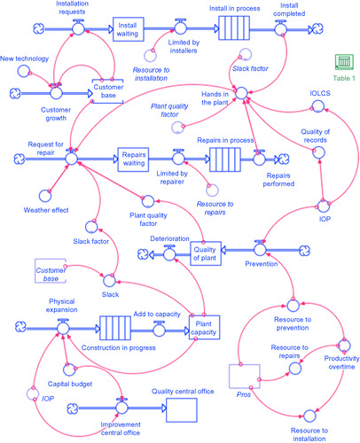
Slack factor: Traditionally 25% of telephone lines in a given installed cable are reserved to replace active lines in case of future failures, but unprecedented demand of the existing customers for additional lines for Internet activity had forced the company to use up the slack lines. Therefore when an active line for any reason had failed, under customer pressure, it was switched to another active line. As expected, this only bought a few days before adding another complaint to the accumulating list of existing ones.
2. Functional organizational structure: Each of one of the interrelated activities captured in the following model was the responsibility of a separate department. All of the reward systems were volume-based not result-oriented. Blame was the common game played artfully by all involved. There was a constant power struggle and fight for additional resources.
3. Increased number of hands in the plant: Competing interest among different functions had increased “hands in the plant.” This, along with poor and irresponsible documentation, undermined the “quality of the records” for each plant and increased the level of malfunctioning. There was a high correlation between the number of hands in a plant for a given period and the number of additional complaints reported.
4. Volume based reward system: Workers were also enjoying record earnings based on overtime pay and took full advantage of the volume-oriented reward system.
The mess was dissolved within three months after a modular design replaced the existing structure where all interdependent activities were given to a neighborhood center with a reward system based on results and customer satisfaction instead of volume. A team of technicians was assigned to a given neighborhood and was told they would receive their full overtime pay if the number of customer complaints for a given period fell below a normal rate. Module managers were given the authority to limit the installation of new lines based on the state and quality of the plant and slack factor at the same time expansion of the plant capacity was oriented more toward the weakest link rather than the convenience of the capacity expansion group. See Chapter 7 for discussion of modular design.
Finally, we do recognize that the main function of a business is to produce a throughput, that is, to generate and disseminate wealth. However, an effective throughput cannot be designed independent of organizational processes that provide the platform and infrastructure for its operation (Figure 6.25). The holistic approach requires that designers explicitly define the parameters of these subsystems and understand the behavioral implication of different designs.
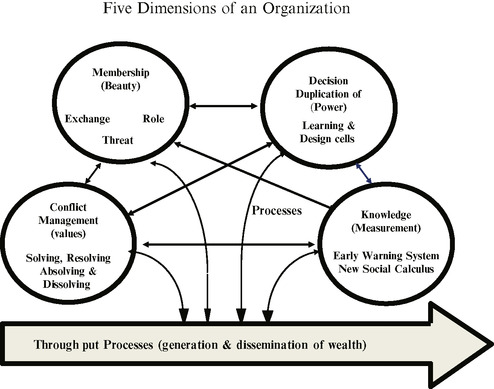
Design parameters and characteristics of organizational processes are basically defined by assumptions and imperatives of the dominant culture or the paradigm in use for each organization. The four organizational processes are very much interdependent and value driven. Together, they define critical attributes of the organizational culture. More often than not, these attributes are produced by default rather than design. Once in place, however, they remain intact during ups and downs of technological change.
Throughput processes, on the other hand, are technologically driven. They explicitly define how the output of an organization is to be produced in the context of a given technology. Uniquely designed for each output, throughput processes are subject to continuous change and improvement.
Since throughputs are redesigned more frequently, there is always a good chance those new generations of throughput designs will become incompatible with more traditional organizational processes already in place. This has been the major cause of the failures, already witnessed, in most re-engineering efforts of recent times. A redesigned throughput process cannot be effectively implemented without proper concern for its compatibility with the existing order — the organizational processes already in place. Usefulness of any model, needless to say, depends on the validity of the underlying assumptions used to develop the operating formulas behind the icons.
6.3.3. Measurement and Learning
The third element of our scheme is the measurement and diagnostic system. The simulation model should provide an online capability to monitor all of the interdependent success factors in the same frame, at the same time, so their relationships can be monitored. This condition is necessary for an effective diagnostic system. The diagnostic system should be able to recognize when the improvement process hits a plateau because this indicates that the system has used up the slacks and that the existing design has exhausted its maximum potential. To achieve an order-of-magnitude change in the system's performance, we need to replace the existing framework and redesign the process. Read-only memory is a critical element of our scheme. We need to incorporate a learning system so that all of our assumptions, expectations, and changes in the design process are recorded in a read-only memory. These entries, which cannot be altered, will be kept intact for learning purposes and future references. See Chapter 7 for discussion and design of learning systems.
..................Content has been hidden....................
You can't read the all page of ebook, please click here login for view all page.