
Chapter 5 -Three Options for Teradata Table Design
“Design is not just what it looks like and feels like. Design is how it works.”
There are Three Options to Teradata Table Design
1. Traditional Teradata using a Primary Index:
80-90% of your tables will use the traditional Teradata design of simply having a Primary Index. These tables will distribute the rows of the table among the AMPs with a consistent and straightforward Hash Formula. The AMPs will sort their rows by the Primary Index value (kind of) and when a user queries the table using the Primary Index value to limit the rows returning it will always be a “Single AMP retrieve”.
2. Partition the table which is called a PPI Table (Partition Primary Index):
Teradata allows a table to be created with a horizontal partition. A PPI table still has a Primary Index that distributes the rows among the AMPs just like a traditional table, but each AMP sorts the data on the partition column. All AMPs will be involved in retrieving an answer set, but each AMP only reads one or more of their partitions thus no longer performing a Full Table Scan.
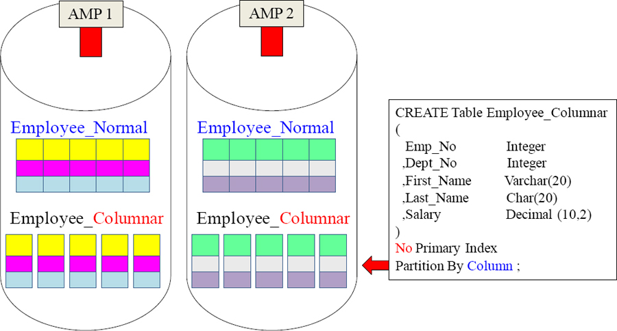
3. A Columnar Design:
In Teradata V14, the system allows for tables to be created in a columnar design. The rows are distributed randomly, but evenly among the AMPs because the table has no Primary Index. Each AMP still owns their own rows, but the rows break each column up into their own separate column container. In other words, if a query only requests a few columns in the query, then the AMP only moves a few small containers into FSG cache. This is considered vertical partitioning.
How Teradata Creates Traditional Tables
CREATE TABLE Employee_Table
( EmpNo INTEGER
,Dept_No INTEGER
,First_Name VARCHAR (12)
,Last_Name CHAR(20)
,Salary DECIMAL (10,2)
) UNIQUE PRIMARY INDEX (EmpNo) ;
When a table is created, the Primary Index is defined. 90% of your tables will use this design. Choosing the best column for the Primary Index is your number one strategy.
Notice the last line of the CREATE Table example above, and you will see that EmpNo is defined as the Primary Index. This means that the rows that are loaded into the Employee_Table will be hashed and distributed to the AMP based solely on the value in the rows EmpNo. The column EmpNo will be responsible for the distribution, and if the column EmpNo is used by the user in the SQL to find a specific employee number (EmpNo), then only one AMP will be contacted to find the row.
Each Table has a Primary Index
CREATE TABLE Employee_Table
( EmpNo INTEGER
,Dept_No INTEGER
,First_Name VARCHAR (12)
,Last_Name CHAR(20)
,Salary DECIMAL (10,2)
) UNIQUE PRIMARY INDEX (EmpNo) ;
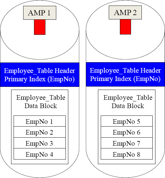
Each traditional Teradata table chooses a column to be the Primary Index. The Primary Index column is used to distribute the rows among the AMPs and it's how each AMP sorts the rows.
When users query a table and use the Primary Index column in their SQL to find a specific EmpNo, only a “Single AMP” is used. The Primary Index is your best friend.
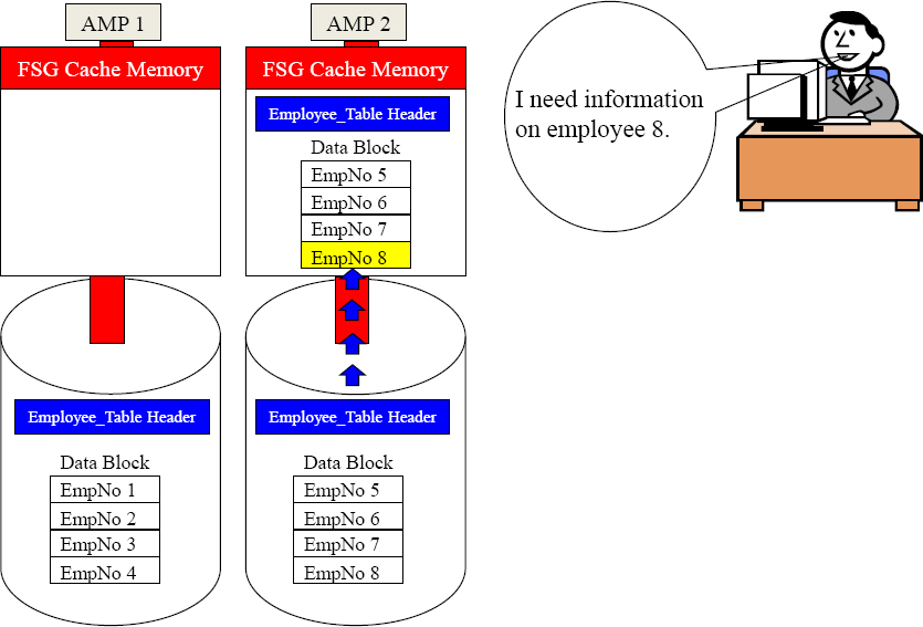
A Query Using the Primary Index is a Single AMP Retrieve
Parsing Engine
Here is the plan AMP 2.
I know you have EmpNo 8 because EmpNo is the Primary Index, and I distributed it there.
Move your Employee_Table header and data block into FSG Cache, and retrieve the row.
Choosing a good Primary Index is paramount. The above example results in only a “Single AMP” being used in the query.
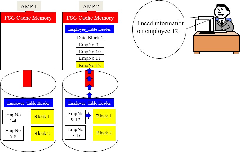
A Primary Index Query uses a Single AMP and Single Block
Parsing Engine
Here is the plan AMP 2.
I know you have EmpNo 12 because EmpNo is the Primary Index.
You should have two blocks. Only Transfer the block holding EmpNo 12 to your FSG Cache, and send me the results.
AMP 2 was contacted and told to only transfer the block that has EmpNo 12. Now, you see the importance of each AMP sorting their rows to limit transferring each block.
How Teradata Creates a PPI Table
CREATE TABLE Order_Table
( Order_Number INTEGER
,Customer_Number INTEGER
,Order_Date DATE
,Order_Total Decimal (10,2)
) PRIMARY INDEX(Order_Number)
PARTITION BY RANGE_N
(Order_Date BETWEEN
date '2013-01-01' AND date '2013-12-31'
EACH INTERVAL ‘1' Month) ;
A Partitioned Primary Index (PPI) table has a Primary Index that distributes the rows among the AMPs, but they are not sorted by the Primary Index. Instead, an AMP is instructed to sort the rows they own by the Partition.
In the above example, the first part of the CREATE Table statement looks just like the previous example, but it is the latter part of the statement that you see the words “Partition By”. This table's rows will still be distributed among the AMPs via the Primary Index of Order_Number, but the AMPs won't sort by Order_Number. Each AMP will sort their rows by the partition which is Month of the Order_Date. Look at the next page to see a visual of the AMPs and their sorting of millions of rows.
PPI Table Sorting the Rows by Month of Order_Date
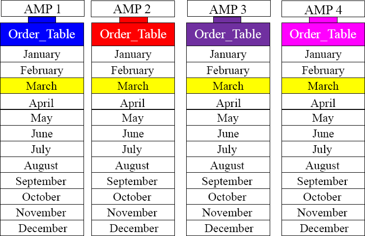
Each AMP above sorts their rows by Month (of Order_Date), so if a user queries and only wants to see the orders placed in March, then each AMP just transfers the blocks with March orders. This is an all AMP retrieve, but each AMP only has to retrieve from a single partition which is the March Partition.
An All AMPs Retrieve By Way of a Single Partition
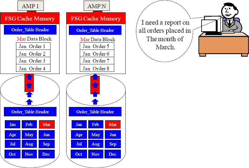
Parsing Engine
Calling all AMPs. Do NOT do a Full Table Scan!
You should each have 12 blocks (one per month). Move your March Partition block into your FSG Cache.
Give me all March Orders.
All AMPs are used to satisfy the query, but each AMP only reads a portion of their rows.
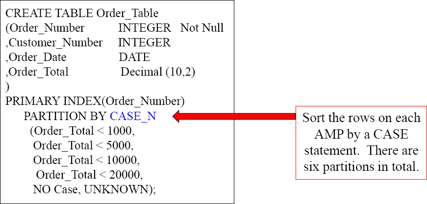
Creating a PPI Table with CASE_N
There are three different types of Partitioning:
1) Simple
2) RANGE_N
3) CASE_N
The above syntax represents the CASE_ N partitioning. If an Order_Total is < 1000, it will go into Partition 1. If an Order_Total is between 1000 and 4999.99, it will go in Partition 2. The NO Case partition is for anything falling through, and the UNKNOWN partition is for NULL values in the Total.
A Visual of Case_N Partitioning
PARTITION BY CASE_N
(Order_Total < 1000,
Order_Total < 5000,
Order_Total < 10000,
Order_Total < 20000,
NO Case, UNKNOWN);
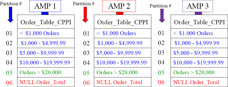
There are six partitions for this table. Orders go into partitions based on Order_Total.
An All AMPs Retrieve By Way of a Single Partition
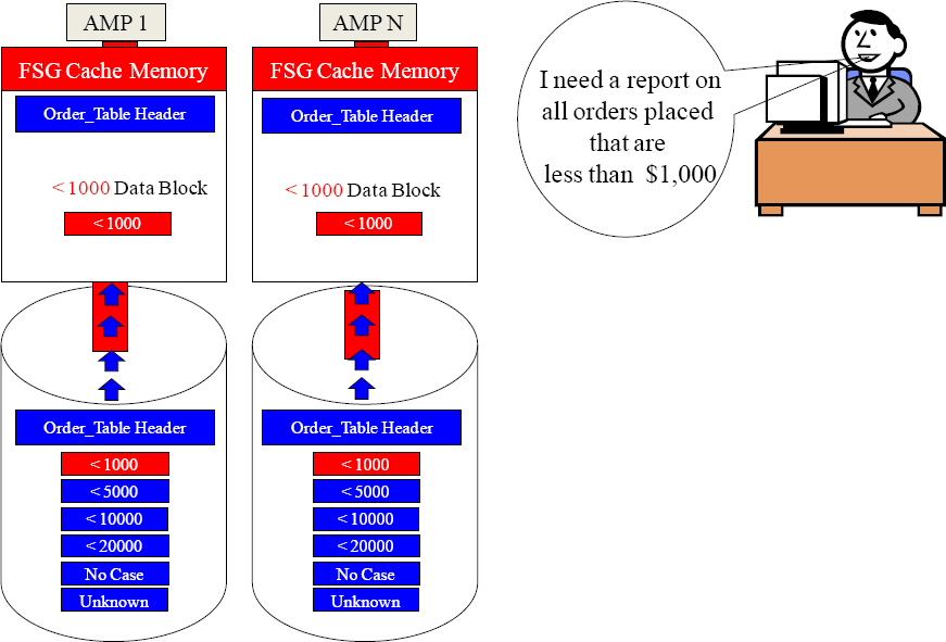
Parsing Engine
Calling all AMPs. Do NOT do a Full Table Scan!
You should each have 6 blocks (one per Case). Move your < 1000 Partition block into your FSG Cache.
Give me all Orders < $1000.
All AMPs are used to satisfy the query, but each AMP only reads a portion of their rows.
What does a Columnar Table look like?
The two tables above contain the same Employee data, but the bottom example is a columnar table. Employee_Normal has 3 rows on each AMP with 5 columns. Employee_Columnar is split into 5 containers, and each container has one column.
A Comparison of Data for Normal Vs. Columnar
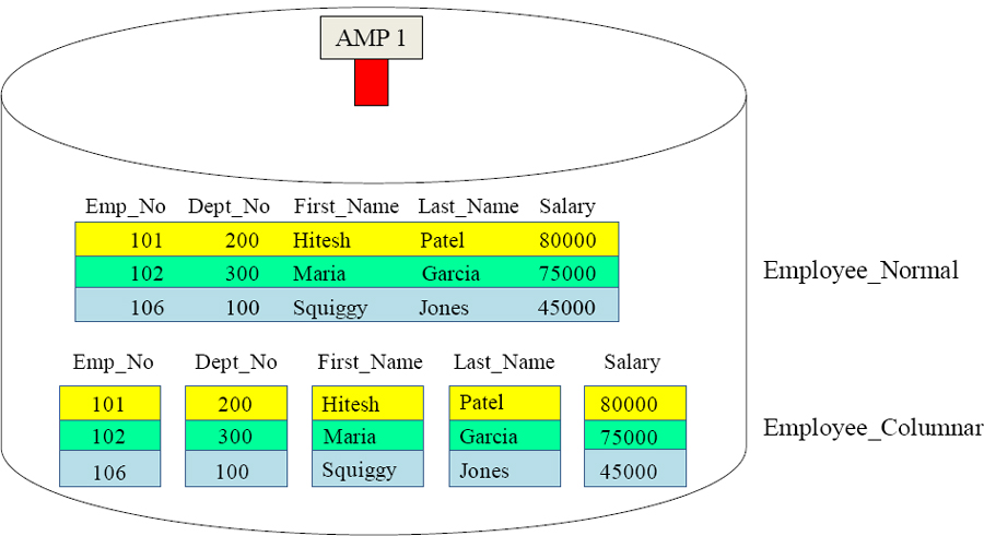
The normal table on top is one block containing three rows and five columns. The columnar table below has five blocks each containing one column of three rows. Columnar tables are better when users query just a few columns and not all columns.
A Columnar Table is best for Queries with Few Columns
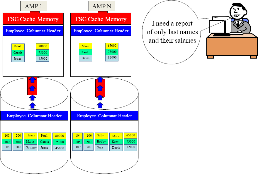
Parsing Engine
Calling all AMPs.
You should each have 5 container blocks in your table named Employee_Columnar. Move only your Last_Name and Salary container blocks into your FSG Cache.
Give me all Last Names and Salaries.
All rows come back, but only two columns. We moved less than half the block volume.
Quiz – How Many Containers are in FSG Cache?
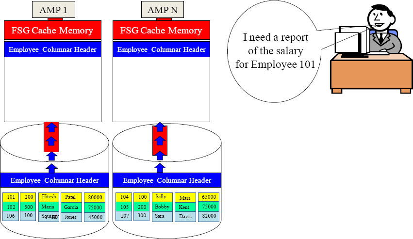
SELECT Salary FROM Employee_Columnar
WHERE EmpNo = 101 ;
There are 1,000 AMPs in the system!
There are no indexes on the table as it is a NoPI table.
How many containers will be placed into FSG Cache to satisfy the query?
____________________
Your mission is to think! Remember that the Parsing Engine does the least work always.
Answer – How Many Containers are in FSG Cache?
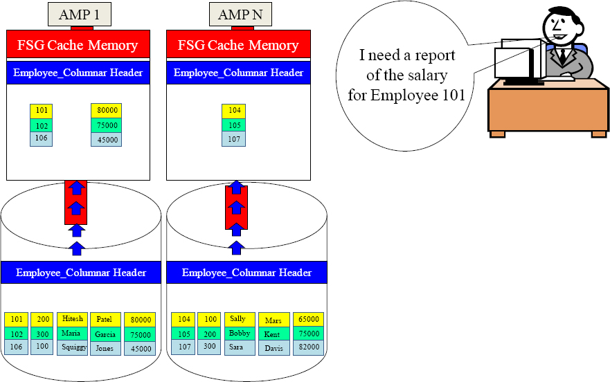
There are 1,000 AMPs in the system!
There are no indexes on the table as it is a NoPI table.
How many containers will be placed into FSG Cache to satisfy the query?
1001
All 1,000 AMPs place only their EmpNo container in FSG Cache, and then the AMP that finds Employee 101 will move their Salary container in. Did you think 2000?
Intelligent Memory (Teradata V14.10)
| Teradata 14.10 utilizes automated, multi-temperature data management into memory management by keeping the very hottest data in memory automatically. | |
| There is no DBA intervention or application changes required. | |
| Teradata Virtual Storage (TVS) temperature measurement is used to determine what data is the hottest | |
| Intelligent Memory is available on all Teradata platforms with Teradata V14.10. | |
| Intelligent Memory is, in addition to Teradata's FSG cache, traditional caching memory. FSG Cache memory is used to store data temporarily to process current queries. Intelligent memory doesn't purge the data in memory but instead keeps it there. | |
| Once TVS temperature monitoring marks data as hottest, it will be kept in memory, and the next time it's brought in for use in any processing, it could stay there for days. |
Above are the features of Teradata V14.10 Intelligent Memory.
Teradata V14.10 Intelligent Memory Gives Data a Temperature
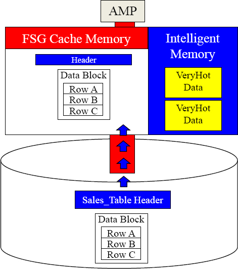
An AMP now has two types of memory. The first is FSG cache, and it is used for processing queries by bringing blocks from disk into FSG cache where processing occurs as it always has.
The second is Intelligent memory, and it is used for VeryHot temperature data. This data stays in memory for days until it cools. It provides the fastest query capabilities on the hottest of data.
Data Dictionary data is VeryHot and so is Tactical sub second query data as well as the most frequently queried tables. Teradata automatically tracks the hottest data blocks and deems their temperature VeryHot. The VeryHot data remains in Intelligent Memory, so queries accessing VeryHot data have no data block movement from disk.
Data deemed VeryHot stays in each AMP's Intelligent Memory
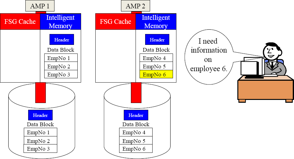
The slowest part of Teradata is moving data from disk to memory. Intelligent memory takes advantage of increased memory in Teradata V14.10 systems. The extra memory is used by each AMP to keep the data deemed VeryHot in Intelligent Memory until the data cools which could be for days.
Intelligent Memory Stays in Memory
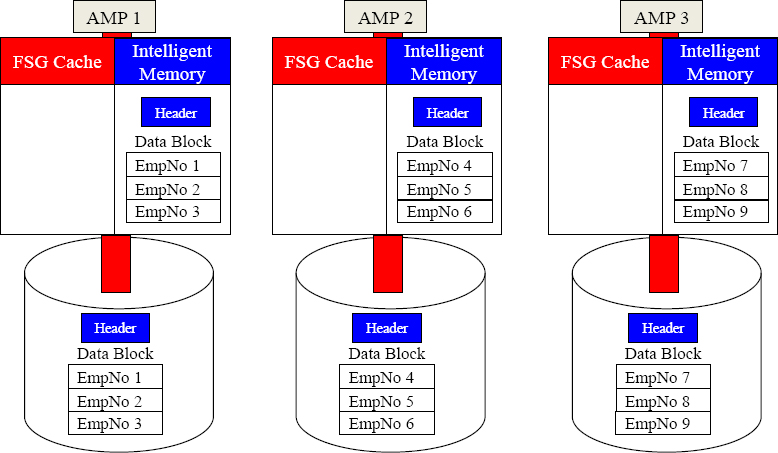
Data that is deemed VeryHot is moved from disk to each AMP's intelligent memory where is stays for up to several days until it cools. Teradata tracks which data is cold, warm, hot, and VeryHot, so the data accessed the most frequently remains available instantly. This is a brilliant strategy by Teradata and will help enormously where speed is the need.
Factors When Choosing Table Design
- How will users use the Primary Index?
- How many rows are in the table?
- How many columns are in the table?
- Will the users do more Full Table Scans or use a WHERE clause to bring back a few rows?
- Will the users require most of the columns on the report or just a subset?
- Will the users perform range queries on a particular column like date?
- How can I best avoid a Full Table Scan?