
Chapter 11 - Explain
“A rule to live by: I won't use anything I can't explain in five minutes.”
EXPLAIN Keywords
| Locking Pseudo Table | Serial lock on a symbolic table. Every table has one. Used to prevent deadlocks situations between users. |
| Locking table for | Indicates that an ACCESS, READ, WRITE, or EXCLUSIVE lock has been placed on the table |
| Locking rows for <type> | Indicates that an ACCESS, READ, or WRITE, lock is placed on rows read or written |
| Do an ABORT test | Guarantees a transaction is not in progress for this user |
| All AMPs retrieve | All AMPs are receiving the AMP steps and are involved in providing the answer set |
| By way of an all rows scan | Rows are read sequentially on all AMPs |
| By way of primary index | Rows are read using the Primary index column(s) |
| By way of index number | Rows are read using the Secondary index –number from HELP INDEX |
| BMSMS | Bit Map Set Manipulation Step, alternative direct access technique when multiple NUSI columns are referenced in the WHERE clause |
| Residual conditions | WHERE clause conditions, other than those of a join |
| Eliminating duplicate rows | Providing unique values, normally result of DISTINCT, GROUP BY or subquery |
| Where unknown comparison will be ignored | Indicates that NULL values will not compare to a TRUE or FALSE. Seen in a subquery using NOT IN or NOT = ALL because no rows will be returned on ignored comparison. |
| Nested join | The fastest join possible. It uses a UPI to retrieve a single row after using a UPI or a USI in the WHERE to reduce the join to a single row. |
EXPLAIN Keywords Continued
| Merge join | Rows of one table are matched to the other table on common domain columns after being sorted into the same sequence, normally Row Hash |
| Product join | Rows of one table are matched to all rows of another table with no concern for domain match |
| ROWID join | A very fast join. It uses the ROWID of a UPI to retrieve a single row after using a UPI or a USI in the WHERE to reduce the join to a single row. |
| Duplicated on all AMPs | Participating rows for the table (normally smaller table) of a join are duplicated on all AMPS |
| Hash redistributed on all AMPs | Participating rows of a join are hashed on the join column and sent to the same AMP that stores the matching row of the table to join |
| SMS | Set Manipulation Step, result of an INTERSECT, UNION, EXCEPT or MINUS operation |
| Last use | SPOOL file is no longer needed after the step and space is released |
| Built locally on the AMPs | As rows are read, they are put into SPOOL on the same AMP |
| Aggregate Intermediate Results computed locally | The aggregation values are all on the same AMP and therefore no need to redistribute them to work with rows on other AMPs |
| Aggregate Intermediate Results computed globally | The aggregation values are not all on the same AMP and must be redistributed on one AMP, to accompany the same value with from the other AMPs |
Explain Example – Full Table Scan
EXPLAIN SELECT * FROM Employee_Table ;
1) First, we lock a distinct SQL_CLASS. “pseudo table” for read on a RowHash to prevent global deadlock for SQL_CLASS.Employee_Table.
2) Next, we lock SQL_CLASS.Employee_Table for read.
3) We do an all-AMPs RETRIEVE step from SQL_CLASS.Employee_Table byway of an all-rows scan with no residual conditions into Spool 1 (group_amps), which is built locally on the AMPs. The size of Spool 1 is estimated with low confidence to be 6 rows (342 bytes). The estimated time for this step is 0.03 seconds.
4) Finally, we send out an END TRANSACTION step to all AMPs involved in processing the request.
-> The contents of Spool 1 are sent back to the user as the result of statement 1. The total estimated time is 0.03 seconds.
When you see all-AMPs RETRIEVE by way of an all-rows scan, that means that Teradata is doing a Full Table Scan and thus it is reading every row in the table. All AMPs are retrieving all the rows they own.
Explain Example – Unique Primary Index (UPI)
EXPLAIN SELECT * FROM Employee_Table
WHERE Employee_No = 2000000;
1) First, we do a single-AMP RETRIEVE step from SQL_CLASS.Employee_Table by way of the unique primary index “SQL_CLASS.Employee_Table.Employee_No = 2000000” with no residual conditions. The estimated time for this step is 0.01 seconds.
-> The row is sent directly back to the user as the result of statement 1. The total estimated time is 0.01 seconds.
If you use the Primary Index column in the WHERE clause, you will most likely get a Single-AMP retrieve by way of the Unique Primary Index. This is the fastest query!
Explain Example – Non-Unique Primary Index (NUPI)
EXPLAIN SELECT * FROM Sales_Table
WHERE Product_ID = 1000 ;
1) First, we do a single-AMP RETRIEVE step from SQL_CLASS.Sales_Table by way of the primary index “SQL_CLASS.Sales_Table.Product_ID = 1000” with no residual conditions into Spool 1 (one-amp), which is built locally on that AMP. The size of Spool 1 is estimated with low confidence to be 2 rows (66 bytes). The estimated time for this step is 0.02 seconds.
-> The contents of Spool 1 are sent back to the user as the result of statement 1. The total estimated time is 0.02 seconds.
If you use the Primary Index column in the WHERE clause, you will most likely get a Single-AMP retrieve. This example utilized a Non-Unique Primary Index (NUPI). It doesn't get much faster than this unless it utilizes a Unique Primary Index (UPI).
Explain Example – Unique Secondary Index (USI)
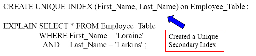
1) First, we do a two-AMP RETRIEVE step from SQL_CLASS.Employee_Table by way of unique index # 12 “SQL_CLASS.Employee_Table.Last_name = ‘Larkins’
, SQL_CLASS.Employee_Table.First_name = ‘Loraine’” with no residual conditions. The estimated time for this step is 0.01 seconds.
-> The row is sent directly back to the user as the result of statement 1. The total estimated time is 0.01 seconds.
Using a UNIQUE Secondary Index (USI) in the WHERE clause will result in a two-AMP Retrieve every time. This is very fast.
Explain Example – Redistributed to All-AMPs
EXPLAIN SELECT E.*, D.*
FROM Employee_Table as E
INNER JOIN
Department_Table as D
ON E.Dept_No = D.Dept_No ;
4) We do an all-AMPs RETRIEVE step from SQL_CLASS.E by way of an all-rows scan with a condition of (“NOT (SQL_CLASS.E.Dept_No ISNULL)”) into Spool 2 (all_amps), which is redistributed by the hash code of (SQL_CLASS.E.Dept_No) to all AMPs. Then we do a SORT to order Spool 2 by row hash. The size of Spool 2 is estimated with low confidence to be 6 rows (294 bytes). The estimated time for this step is 0.01 seconds.
5) We do an all-AMPs JOIN step from SQL_CLASS.D by way of a RowHash match scan, which is joined to Spool 2 (Last Use) by way of a RowHash match scan. SQL_CLASS.D and Spool 2 are joined using a merge join, with a join condition of (“Dept_No = SQL_CLASS.D.Dept_No”).
Data is often redistributed on a Join to ensure that the matching rows are on the same physical AMPs in Spool. If you see the word redistributed, then data is being moved!
Explain Example – Row Hash Match Scan
EXPLAIN SELECT E2.*, D.*
FROM Employee_Table2 as E2
INNER JOIN
Department_Table as D
ON E2.Dept_No = D.Dept_No ;
4) We do an all-AMPs JOIN step from SQL_CLASS.D by way of a RowHash match scan, which is joined to SQL_CLASS.E2 by way of a RowHash match scan. SQL_CLASS.D and SQL_CLASS.E2 are joined using a merge join, with a join condition of (“SQL_CLASS.E2.Dept_No = SQL_CLASS.D.Dept_No”). The result goes into Spool 1 (group_amps), which is built locally on the AMPs. The size of Spool 1 is estimated with low confidence to be 8 rows (728 bytes). The estimated time for this step is 0.04 seconds.
5) Finally, we send out an END TRANSACTION step to all AMPs involved in processing the request.
When you see the words Row Hash Match Scan, then the matching rows are on the same physical AMP in Spool and the join takes place. This is what you want to see for Joins, and it is even better when data isn't moved beforehand.
Explain Example – Duplicated on All-AMPs
EXPLAIN SELECT E.*, D.*
FROM Employee_Table as E,
Department_Table2 as D
WHERE E.Dept_No = D.Dept_No;
4) We execute the following steps in parallel.
1) We do an all-AMPs RETRIEVE step from SQL_CLASS.d by way of an all-rows scan with a condition of (“NOT (SQL_CLASS.d.Dept_No IS NULL)”) into Spool 2 (all_amps), which is duplicated on all AMPs. Then we do a SORT to order Spool 2 by the hash code of (SQL_CLASS.d.Dept_No). The size of Spool 2 is estimated with low confidence to be 16 rows (752 bytes). The estimated time for this step is 0.01 seconds.
Data is often redistributed on a Join to ensure that the matching rows are on the same physical AMPs in Spool. If you see the word redistributed, then data is being moved! This means that the smaller table (usually) is duplicated on each AMP. The Parsing Engine decided that this was a less costly approach than redistributing the data. This is sometimes called a Big Table/Small Table Join.
Explain Example –Low Confidence
EXPLAIN SELECT * FROM Addresses;
1) First, we lock a distinct SQL_CLASS. “pseudo table” for read on a RowHash to prevent global deadlock for SQL_CLASS.Addresses.
2) Next, we lock SQL_CLASS.Addresses for read.
3) We do an all-AMPs RETRIEVE step from SQL_CLASS.Addresses by way of an all-rows scan with no residual conditions into Spool 1(group_amps), which is built locally on the AMPs. The size of Spool 1 is estimated with low confidence to be 2 rows (114 bytes). The estimated time for this step is 0.03 seconds.
4) Finally, we send out an END TRANSACTION step to all AMPs involved in processing the request.
-> The contents of Spool 1 are sent back to the user as the result of statement 1. The total estimated time is 0.03 seconds.
The EXPLAIN plan estimates 2 rows, but there are actually 5 rows coming back. When the Explain plan shows low confidence, it is often because there are no COLLECT STATISTICS on the table, so the PE estimates. Statistics collection is often done by the DBA. The next slide will COLLECT STATISTICS and retry the query.
Explain Example – High Confidence
![]()
COLLECT STATISTICS on Addresses
COLUMN Subscriber_No ;
![]()
EXPLAIN SELECT * FROM Addresses;
3) We do an all-AMPs RETRIEVE step from SQL_CLASS.Addresses by way of an all-rows scan with no residual conditions into Spool 1 (group_amps), which is built locally on the AMPs. The size of Spool 1 is estimated with high confidence to be 5 rows (285 bytes). The estimated time for this step is 0.03 seconds.
4) Finally, we send out an END TRANSACTION step to all AMPs involved in processing the request.
The EXPLAIN plan now estimates 5 rows and shows High confidence because there are COLLECT STATISTICS on the table. If No Statistics are on the table, the Parsing Engine will make an estimate after sampling a Random AMP.
Explain Example – Product Join
EXPLAIN SELECT *
FROM Student_Table S, Course_Table C, Student_Course_Table SC
WHERE s.Student_Id = sc.Student_Id ;
6) We do an all-AMPs JOIN step from SQL_CLASS.C by way of an all-rows scan with no residual conditions, which is joined to Spool 2 (Last Use) by way of an all-rows scan. SQL_CLASS.C and Spool 2 are joined using a product join, with a join condition of (“(1=1)”). The result goes into Spool 1 (group_amps), which is built locally on the AMPs. The size of Spool 1 is estimated with low confidence to be 96 rows (7,584 bytes). The estimated time for this step is 0.05 seconds.
The product join in step 6 is using (1=1) as the join condition where it should be a merge join. Therefore, this is a Cartesian product join. A careful analysis of the SELECT shows a single join condition in the WHERE clause. However, this is a three-table join and should have two join conditions. The WHERE clause needs to be fixed and by using the EXPLAIN, we have saved valuable time.
Explain Example – BMSMS
EXPLAIN SELECT * From Employee_Table as E
WHERE Salary = 36000.00
AND Dept_No = 400;
3) We do a BMSMS (bit map set manipulation) step that builds a bit map for Employee_Table by way of index # 4 Salary = 360000.00” which is placed in Spool 2. The estimated time for this step is 0.01 seconds.
4) We do an all-AMPs RETRIEVE step from E by way of index # 8 E.Dept_No= 400” and the bit map in Spool 2 (Last Use) with a residual condition of (“E.Salary = 36000.00”) into Spool 1 (group_amps), which is built locally on the AMPs. The size of Spool 1 is estimated with low confidence to be 50 rows (4620 bytes). The estimated time for this step is 0.02 seconds.
BMSMS (Bit Map Set Manipulation Step) is an excellent way to process large tables. This basically occurs when multiple columns are ANDed together with each Column being a Non-Unique Secondary Index (NUSI). This usually won't happen unless STATISTICS were collected on the table.
Explain Terminology for Partitioned Primary Index Tables
“A single partition of” means that an AMP will access a single partition of a table. This is called Partition Elimination. Only a small slice of the table is read.
“N partition of” means that an AMP will access N partitions of a table. This is called also considered Partition Elimination. The smaller the number N is the faster the query will be compared to the usual Full Table Scan.
“SORT to partition Spool m by RowKey” means the spool is to be sorted by RowKey, which constitutes the Partition Number and the Hash of the Primary Index. This is done usually for a Join.
“A RowKey-based” means an equality join on the RowKey, which is similar to the Row Hash Match Scan for Non-PPI tables. The Join is taking place.
“Enhanced by dynamic partition” means a join condition where dynamic partition elimination has been used.
Partitioned Primary Index (PPI) tables are tables that are not sorted by Row-Hash on each AMP, but instead sorted first by the Partition. This is designed to eliminate full table scans on Range Queries. When the explain shows Partition Elimination, then a Full Table Scan is NOT being performed which is the entire purpose of PPI Tables.
Explain Example – From a Single Partition
EXPLAIN SELECT * FROM Order_PPI
WHERE Order_Date = ‘1998-05-04’ ;
3) We do an all-AMPs RETRIEVE step from a single partition of SQL_CLASS.Order_PPI with a condition of (“SQL_CLASS.Order_PPI.Order_Date = DATE ‘1998-05-04’”) with a residual condition of (“SQL_CLASS.Order_PPI.Order_Date = DATE ‘1998-05-04’”) into Spool 1 (group_amps), which is built locally on the AMPs. The size of Spool 1 is estimated with no confidence to be 1 row (41 bytes). The estimated time for this step is 0.02 seconds.
The above example uses all-AMPs, but each AMP only reads a single partition. This is as good as it gets with a Partition Primary Index (PPI) Table.
Explain Example – From N Partitions
EXPLAIN SELECT * FROM Order_PPI
WHERE Order_Date BETWEEN '1998-05-01' and '1998-05-31' ;
3) We do an all-AMPs RETRIEVE step from 31 partitions of SQL_CLASS.Order_PPI with a condition of (“(SQL_CLASS.Order_PPI.Order_Date <= DATE ‘1998-05-31’) AND (SQL_CLASS.Order_PPI.Order_Date >= DATE ‘1998-05-01’)”) into Spool 1 (group_amps), which is built locally on the AMPs. The size of Spool 1 is estimated with no confidence to be 2 rows (82 bytes). The estimated time for this step is 0.03 seconds.
4) Finally, we send out an END TRANSACTION step to all AMPs involved in processing the request.
The above example uses all-AMPs, but each AMP only 31 partitions. This has eliminated reading the entire table and dramatically improved the performance on Range Queries like the example above.
Explain Example – Partitions and Current_Date
EXPLAIN SELECT * FROM Order_PPI
WHERE Order_Date = Current_Date ;
3) We do an all-AMPs RETRIEVE step from a single partition of SQL_CLASS.Order_PPI with a condition of (“SQL_CLASS.Order_PPI.Order_Date = DATE ‘2012-06-18’”) with a residual condition of (“SQL_CLASS.Order_PPI.Order_Date = DATE ‘2012-06-18’”) into Spool 1 (group_amps), which is built locally on the AMPs. The size of Spool 1 is estimated with no confidence to be 1 row (41 bytes). The estimated time for this step is 0.02 seconds.
The above example uses all-AMPs, but each AMP reads only one partition. What is different about this is the improvement that Teradata has made to Current_Date. This happened in Teradata V12 and is a welcomed addition.