
CHAPTER
12
Star Schema Designs for Sales Analysis
Suppose that ABC Corporation has built the data warehouse depicted in Chapter 11. Excited about the opportunity to get meaningful sales analysis information, the eastern regional sales manager has approached the IS department to see how and when the data would be available. The IS department, knowing that nothing is as simple as it seems, gathered some specific requirements. After a review of the real requirements, it was obvious that the sales manager did not need access to the entire warehouse. In fact, that would be too much information and ultimately result in confusion and dissatisfaction. IS decided the best solution was to develop a departmental data warehouse (or data mart).
The data warehouse stores all the atomic data necessary to capture all-important historic details. The data mart provides a mechanism to take a slice of this data for easy analysis by the end user. Each data mart usually takes a portion of the data warehouse and is designed to handle the needs of a specific department or part of the enterprise.
As pointed out in the previous chapters, a data warehouse is generally developed one subject area at a time. This chapter will briefly discuss possible star schema structures for a departmental warehouse containing the subject area of sales analysis to be transformed.
The purpose of the designs in this chapter is to provide an example of a department-specific data warehouse (or data mart) that could be developed from the data warehouse. Each enterprise may choose to modify this sales analysis departmental warehouse to meet its own specific needs. The models are presented in a standard star schema format to allow for multidimensional analysis. A star schema is a database design that contains a central table, called a fact table, with relationships to several look-up tables called dimensions. When the schema is diagrammed, it often forms a pattern resembling a star, thus the name star schema.
The models in this chapter will allow the DSS analyst to answer questions such as the following:
- What was the sales volume for a product during a specific time period?
- What was the sales volume for a category of products for a specific time period?
- How much of each product did various customers buy?
- How much of each product category did a selected customer buy?
- How much are the sales reps selling? To whom are they selling?
- Which products or product categories are they selling?
- When were sales the best? When were sales the worst?
- During those times who was buying and who was making the sale?
- Which products and/or customers are most profitable?
The specific schemas presented in the following pages include the following:
- Sales analysis data mart design
- Transaction-oriented sales data mart
- Sales performance data mart
- Product analysis data mart design
Continuing with the example, the requirements analysis determined that the eastern region sales manager needs to see sales information by product, customer, sales representative, and geographic area. All this information must be available for analysis over daily, weekly, monthly, quarterly, and yearly time periods. In addition, the sales manager needs the ability to view information at a transaction level on an occasional basis when supporting detail is required.
Figure 12.1 shows a star schema that allows sales to be analyzed many different ways. The diagram shows a simple database star schema containing a central fact table and several dimension tables. The fact table is CUSTOMER_SALES, which contains all the keys to the various dimensions and columns to hold the data to be reported (sometimes called measures). This table provides summarized extracts from the data warehouse to show sales via each of the desired dimensions. The dimensions by which the facts can be queried are CUSTOMERS, CUSTOMER_DEMOGRAPHICS, INTERNAL ORGANIZATIONs, SALES_REPS, ADDRESSES, PRODUCTS, and TIME_BY_DAY. This schema will likely be summarized and loaded on a daily basis so that current data is available every 24 hours. This means the level of granularity is fairly precise because the data is captured daily.
Figure 12.1 Sales analysis star schema.

The information in the CUSTOMER_INVOICES table is the result of transforming the data warehouse table CUSTOMER_INVOICES and its related tables (see Figure 11.1) into an effective data mart design. In order to allow the sales manager (or any DSS analyst) to use a multidimensional analysis approach, the data in the data warehouse is transformed into a (star) schema that is simple to query and performs well.
The key to the fact table is the combination of the various dimension keys: product_id, sales_rep_id, customer_id, customer_demographics_id, internal_organization_id, address_id and day_id. The information from the data warehouse summarizes each invoice and stores the resulting invoice sum-marizations in the fact table, partitioned by the combination of these dimensions. In other words, there would be a record in the CUSTOMER SALES fact table for every combination of the dimensions that has historically occurred.
If analysts wanted to see the resulting detailed transactions for a particular query, they could drill through to the main data warehouse by using the selected dimensions of the query as the parameters to the query to the data warehouse. Many data warehouse tools provide the facility of automatically passing the parameters of a query on a data mart to the data warehouse, in order to query the transactions that made up the summarized data.
The columns quantity, gross sales, and product_cost are the measures on which summaries and trend analysis will be done. The quantity column represents the actual product quantity that was invoiced, and it is from the INVOICE ITEM quantity attribute in the invoices data models from Chapter 7. The gross sales is the summary of the extended amounts (the INVOICE ITEM quantity * amount) for all the invoice items plus or minus any adjustments related to that invoice item, and it is also sourced from the INVOICE ITEM entity. The product cost is the product cost and may be calculated by using information from the PRODUCT COST COMPONENT models in Chapter 2 (V1:3.8). If actual costs are desired, the formulas can be much more complicated, and cost data may be gathered from the order models (to capture the cost of the invoice items), the shipment models (to capture the costs of shipments), and the work effort models (to capture the cost of producing products).
Data transformations that occur from the data warehouse to the data mart include summarizing the data (there could be several sales in the same day for the same dimensions), adding derived data, such as the gross invoice amount, and determining product costs. There could also be restrictions on the data selected. For example, as previously indicated, the process to extract the warehouse data may include customer invoice data only for particular internal organizations, such as certain departments or divisions. This would be done by limiting the selection process to specific organizations. Other possible restrictions could be on sales representatives or customers, or on a date-range basis. The particular algorithm used must be based on the specific business analysis requirements of the enterprise using the data.
During the user interviews, the IS department learned that sales for each bill-to customer were desired. The sales manager, however, was not interested in historical changes to customer names, so the customer_name field is stored in the CUSTOMERS dimension table along with customer_id. The data selected from the warehouse into this table should be the most current data available on each customer.
The star schema shows a relationship to CUSTOMER, which is a subtype of PARTY ROLE. CUSTOMERs may also be further subtyped to define more specific roles such as BILL TO CUSTOMER, SHIP TO CUSTOMER, or END USER CUSTOMER. Because this data mart design is for INVOICE ITEMs, the customer that is represented is the bill-to customer. Additional, separate dimensions may be needed to show the ship-to customer or the end user customer if this information is needed. Ship-to information would be extracted using the relationships from the invoice item to the shipment item.
The data mart design could show ship-to and bill-to customers within a single dimension (as levels within the dimension); however, because there is a many-to-many relationship between bill-to customers and ship-to customers, the designer may want to have separate dimensions of a ship-to customer and a bill-to customer.
Customer Demographics Dimensions
To allow the analyst to get more detail on the demographics behind customers, the CUSTOMER_DEMOGRAPHICS table is included. The data for this dimension table can be directly extracted from the CUSTOMER DEMOGRAPHICS data table found in the enterprise data warehouse.
This table stores a record for each combination of the values for each of the fields in the table. For example, the table could store a credit_rating of “AAA,” marital_status of “married,” and an age of “20–25.” Notice that age uses a range of ages in order to limit the possibilities to a reasonable size instead of allowing a number for each age year.* This would represent a unique row in the CUSTOMER_DEMOGRAPHIC dimension table that could be related to the CUSTOMER_INVOICES fact table.
If the analyst is interested in seeing sales data for all customers within an age of “20–25” that could be done with this data using a restrictive query against CUSTOMER_DEMOGRAPHICS (e.g., select all customer IDs where the age is “20–25”). The same approach could be used to gather data based on marital_status or credit_rating as well.
In order to get meaningful information, the sales manager did indicate a need for demographic data as it was when the sale was made. It does not matter what age the customer is this month. The important information is what age was the customer last year when the sale was closed. In order to provide this level of detail, the CUSTOMER_DEMOGRAPHICS table was built using the columns age, marital_status, and credit_rating. Note that age and marital_status are optional columns because not all customers are people (they could be organizations). The column credit_rating may apply to both people and organizations; however it is also optional as it may not be known.
In the enterprise warehouse, the key to the CUSTOMER_DEMOGRAPHICS table is customer_id and snapshot_date. The data warehouse stores all the changes to customers' demographics. This data mart is interested in demographics only as it applies to invoices. Therefore, the table is loaded by extracting the appropriate snapshots of the demographics as they apply to each invoice. The table could be loaded by extracting the demographics of each customer as applied at the time of each invoice and creating a relationship to the existing CUSTOMER_DEMOGRAPHICS dimension instance or inserting records in the CUSTOMER_DEMOGRAPHICS dimension whenever there is a new combination.
Another question the DSS analyst may need answered is this: What was the sales volume attributed to each sales representative during a certain time period? Also, who was the sales manager who managed the salesperson and was responsible for the sale? To answer these needs, the sales_rep_id and manager_rep_id columns are included as part of the key to CUSTOMER_INVOICES and are the key to the dimension SALES_REPS. The unique combination of the sales rep and manager allows querying on either of these attributes in order to analyze performance.
In the data warehouse, each SALES_REP has a recursive relationship to manager using the recursive relationship and linking the manager_rep_id to see who the sales reps are for that manager or, conversely, seeing who the manager of the sales rep is. The SALES_REPs is stored as a relationship to CUSTOMER_INVOICES. This information is extracted into the data mart and added to the SALES_REPS dimension. The details about a particular rep, including his or her name, are included in the dimension table SALES_REPS. This table corresponds to the SALES_REPS table in the warehouse. The only possible restriction to consider when populating this table would be to select only those reps that are involved in the required sales data. If the warehouse table is small, copying the entire table may be simpler and pose no performance impact. (Note that the definition of “small” varies from one enterprise to another.)
According to the data model, there may be more than one sales representative for an invoice. In these cases, the invoice amounts, quantities, and costs would need to be appropriately split (according to the percentage credit that each salesperson received, as shown in Figure 7.2) to accommodate for correct credit to each sales representative and manager.
Internal Organizations Dimension
Analysts may also want to analyze sales by different internal organizations to assess performance of various subsidiaries, departments, divisions, and so on. The INTERNAL ORGANIZATION dimension allows such analysis.
This data would come from the internal_organization_id and internal_organization_name fields stored in the INTERNAL ORGANIZATIONS dimension table of the data warehouse.
Another component, or dimension, commonly required in DSS and multidimensional analysis is geographic area, region, or location. For example, the eastern region sales manager needs to know sales volume not only by the various geographic areas, but also by the various customer locations or sites. In some cases, it may be critical to know the actual address where sales were made. This will provide the region with information to assess how well different products are selling at various customer locations.
The address_id columns and the ADDRESSES dimension will provide that information for this model. This data is extracted from the warehouse tables CUSTOMER_ADDRESSES and GEOGRAPHIC_BOUNDARIES. The values for city_name, state_abbrv, and country_name will be extracted from the warehouse table GEOGRAPHIC_BOUNDARIES using the column geo_id. As with customer and sales rep data, the only restriction to consider would be to pull only addresses referenced by the selected sales data.
Also dropped from the ADDRESSES table was the customer_id column as a way to identify that the address is for a particular customer (a CONTACT MECHANISM such as a POSTAL ADDRESS may be used by many PARTYs). Because the identifiers for an address are unique and the characteristics of an address rarely change, it was determined (through user interviews) that this dimension needed unique address records only. In other words, the extraction process from the enterprise warehouse needs to pull information for a particular address_id only once, regardless of how many customers are associated with it. This serves to save some space in the departmental warehouse because redundant data is eliminated. Because there is a many-to-many relationship between customers and their addresses, having separate dimensions provides the best flexibility to handle either customer analysis or location analysis.
Notice that the ADDRESSES table includes not only city, state, country, and postal codes but also address_linel and address_line2. This allows the regional sales manager to compare sales for a single customer that may have several locations within the same city. While some DSS analysts may be interested in performance at specific customer locations, others may be more interested in grouping sales by the large geographic areas like city, state, and country; both levels of detail are included.
The PRODUCTS table provides description and category information about the various products that have been sold. Using this dimension, the DSS analyst can determine product sales by product or product category for higher-level analysis. The data in this table is a direct extract or copy of the PRODUCTS table found in the enterprise warehouse model.
The data model in Chapter 3, Figure 3.2, shows that a product may be categorized into more than one category. The current warehouse and this data mart determined that it would select only the primary categorization for the product (as indicated by the primary_flag attribute in the PRODUCT CLASSIFICATION CATEGORY entity in Figure 3.2). If it was necessary to store products in many categories, then the product_id and product_category_id would both need to be the keys to the CUSTOMER_SALES fact table.
An accepted standard in the industry is that most star schema designs will have a time dimension. To accommodate this, the dimension table TIME_BY_DAY is used to store various time periods. It includes fiscal_year, quarter, month, and week and day. In this way, the data in the warehouse can be accessed and summarized to accommodate any of these time periods, not just a single period such as year. Table 12.1 contains examples of the data that could fill the TIME_BY_DAY table.
Table 12.1 Time Period Data
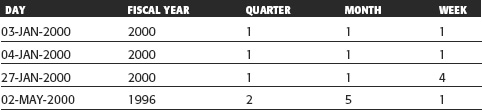
As indicated by the data, the table key, day_id, references the day of the invoice in the fact table. These dates are then associated with the appropriate year, month, quarter, and week. What dates are loaded into this table are again dependent on the time periods over which the enterprise wishes to conduct analysis.
At this point, it should be noted that this time data could mean several things depending on the rules of the enterprise. The table can be used to store organizationally defined time periods. Because many businesses operate on a fiscal year basis, the column for year is called just that: fiscal_year. This allows analysts to work within the bounds of their companies' standard time frames without too much confusion. If the year stored was only a calendar year, confusion could occur when interpreting the data and trends as there would be a mismatch between the time IDs in the dimension table and the time periods expected on company reports. A column for calendar year could be added if both year values are needed for analysis. Other extensions could be made to the model to categorize days into other classifications such as work days, weekends, or holidays.
Using this construct, it is possible to summarize the detailed data in CUSTOMER_SALES by the time element day. It could be summarized by fiscal year so that annual trends could be observed or by month so that the trends within a year could be observed or seasonal trends could be analyzed (e.g., compare gross sales for June, July, and August, for 1995 through 2000). Likewise, summary data by quarter or week could also be constructed. This would be done by selecting data associated with time ID values that have a particular year, month, or week (the actual mechanics of this will vary according to the DSS tool being used). This model is very flexible because one time dimension table could be used to produce many different summaries.
Note that this may or may not provide fast query retrieval, depending on many factors such as the DBMS and amount of data. If performance becomes an issue, then separate tables could be constructed to hold data summarized by the various time periods. For example, a highly summarized table containing this sales data by year could be built simply by substituting a TIME_BY_DAY dimension with a TIME_BY_YEAR dimension. Then a different time dimension table would be required that simply contained the list of years available. (If this was done, then the quantity, gross_sales, and product_cost fields would represent the sum of those values over a year's worth of invoices.) Depending on the needs of the enterprise, a weekly, monthly, or yearly data mart may be used in lieu of the daily data mart, in order to improve performance and save space.
Transaction-Oriented Sales Data Mart
Is a data mart with a granularity level of individual transactions an acceptable data mart design? The data warehouse stores the individual transaction data, so is it necessary to bring these transactions into a data mart because it can be viewed from the data warehouse? With the drill-through capabilities that exist to map back to the original transactions in the warehouse, is it necessary to store these transactions at the data mart level also? Perhaps a particular department just wants to have access to its own invoice transactions and be able to slice and dice these transactions easily by various dimensions.
Suppose we modified the previous data mart design to maintain the data at a lower level of granularity, namely at a transaction level. Figure 12.2 provides an example of this model. The model from Figure 12.1 has been modified by changing the key to invoice_id and invoice_item_id; the foreign keys to the dimension tables in this design are not part of the key to the fact table. (This will be the only fact table in Volume 1 and Volume 2 that does not have all of the foreign keys as part of the key to the fact table.)
Figure 12.2 Transaction-oriented sales data mart.

On the surface it looks as if it is just a finer granularity for sales analysis. There is the added advantage of being able to view invoices at a summary level and then drill down until one gets to the individual transaction. Complications can occur when showing a star schema at a transaction level. Because the transaction needs to be kept intact and some of the relationships for the transaction may involve complex relationships, some information may not be able to be stored correctly.
For example, as shown in the invoices data model, there may be more than one salesperson for the invoice and each received a different percentage for the invoice. This is recorded in the data warehouse design of Figure 11.2, allowing many SALES_REPS for the CUSTOMER INVOICES table. This structure is not supported by a star schema because a star schema is defined by one-to-many relationships from the dimension to the fact table. The truth is that there can be many SALES_REPS for each CUSTOMER_INVOICES instance. Figure 12.2 has simplified the constraint of many salespeople by showing a single salesperson; however, it is not completely accurate.
The previous model, Figure 12.1, took care of this by allocating each salesperson's percentage to each salesperson and transforming the amount in the fact table's measures appropriately. This could be done because the fact instances represent summarized amounts. On a transaction basis, though, this is harder to do. Each transaction could be split into multiple transactions to accommodate the various salespersons. This could double or triple the number of transactions, a number that already may be quite large. If this is done it also may be confusing because the same transaction is stored multiple times. For instance, when counts of transactions are queried, the results may be misleading.
This example shows a key consideration when designing the data warehouse and data marts. The data warehouse is designed to capture the atomic transactions and their history. This may mean capturing data in non-star schema data structures because more complex relationships may be required, such as many-to-many relationships or recursive relationships.
The data mart is designed to capture data in a very easy-to-query and performance-oriented fashion. The star schema format is an example of a data structure that best meets these needs because it is very easy to slice and dice the information in this simple structure; due to its simple data structure, it can be more easily performance optimized.
Thus, the remainder of the universal data mart designs presented in the rest of this book will not be based on granularity of transactions. They will be based on measures that relate to the combination of the dimensions shown for the fact table.
Variations on the Sales Analysis Data Mart
There may be several variations on the star schema design represented in Figure 12.1. Depending on the business questions that need to be answered, the star schema design may vary.
Variation 1: Sales Rep Performance Data Mart
An example of a sales analysis data mart that may have very specific goals is one to measure salesperson performance. Take, for example, the need to analyze the performance of sales reps on a monthly basis. This may be done by the previously mentioned regional sales manager or, in other enterprises, by a human resources manager. These managers may need to evaluate the performance of the sales reps that report to them or develop and monitor sales incentive plans. They generally do not care what products are being sold, nor do they care about customer demographics. Their concern is sales performance and perhaps how much is sold to various customers to determine how diverse the sales rep's market is. To answer these needs, the table SALES_REP_SALES (see Figure 12.3) was designed. This table provides presummarized data by sales rep, customer, and address, by month. For example, suppose the questions that are needed are the following:
- What was the sales volume for a specific sales rep over the last 12 months?
- Which customer bought the highest volume through a particular sales rep for a specific month?
- What was the distribution of sales across a sales rep's customers?
- How much does each sales rep sell across each of his or her assigned states?
- Within each state, which city had the greatest volume for a sales rep?
Figure 12.3 Sales rep performance.

To answer these questions, the model in Figure 12.3 may be the best sales analysis star schema for this application. This star schema may be in lieu of the star schema in Figure 12.1, or it may be in addition to the star schema in Figure 12.1. It may be in addition to the previous star schema because a more summarized version of the star schema may be needed for quicker access. Another reason is that different departments may have different needs regarding access to the data, so there may be several different data mart designs to meet each department's needs. They all, however, should extract data from the same company-wide data warehouse, so that one consistent, integrated source of decision support data can feed many data mart designs.
Notice that there is no longer a PRODUCT dimension table because the table CUSTOMER_REP_SALES is a summarization of data about the performance of the sales reps, regardless of the individual products. Customer demographics are also deemed unimportant, and the CUSTOMER_DEMOGRAPHICS dimension has also been dropped. This table then represents a slightly higher level of summarization than the previous ones because two of the dimensions have been eliminated. The measures quantity and product cost have also been dropped because their values are dependent on product and cannot be summarized correctly in this context.
In this star schema, there is a slight variation in the time dimension table. It is now summarized by month. When the sales manager was interviewed by the IS department, it became clear that daily information was not required to answer the questions posed; however, a monthly view of the data would be most useful. Therefore, the fact table has a column (month_id) that contains the ID to uniquely identify a specific month within the enterprise's fiscal year. This is matched in the time dimension table.
Because the data is to be summarized only by month, the time dimension needs only the columns month, quarter, and fiscal_year. The column week is no longer needed as it makes no sense in a monthly summary view of the data. Another point to note is that summarizing data to the monthly level also represents another higher level of summarization.
Thus, this table can provide the DSS analyst or department manager with another very flexible means of viewing the data.
Variation 2: Product Analysis Data Mart
Suppose a product analyst for ABC Corporation needs information to assess product performance. The information will be used to make strategic decisions on product offerings for various geographic areas. Interviews with the analyst determine that specific customer, customer address, or customer demographic information is unimportant for this type of analysis. It is also determined that monthly summaries will provide an appropriate level of granularity.
Figure 12.4 shows a schema containing PRODUCT_SALES as the central fact table. This is considered more highly summarized because it contains fewer dimensions than the previously discussed tables and because records are summarized by month. Thus, this table can be used to hold presummarized data for product sales by geographic area by month. While previous tables also included customer and sales rep information, this one does not (as the analysis indicated it was not required). Thus, the columns sales_rep_id, customer_id, and address_id are not included in this table. The only dimensions tables needed in this schema are GEOGRAPHIC_BOUNDARIES, PRODUCTS, and TIME_BY_MONTH.
Figure 12.4 Product analysis star schema.
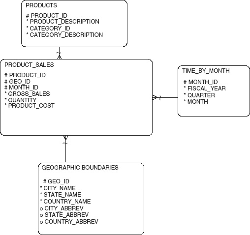
The measures in this table are again quantity, gross_sales, and product_cost. Data in this table could be created by summing all the information in CUSTOMER_INVOICES by product_id, city_name (from the ADDRESSES dimension), month, and year. The cities selected would be referenced by a new column, geo_id. As in the previous examples, this data could also be taken directly from the main warehouse by selecting and summing data from the data warehouse CUSTOMER_INVOICES table for the products of interest. An additional restriction on the data extracted would need to be made through a join to CUSTOMER_ADDRESSES with a summarization based on the city name via the column geo_id.
Geographic Boundaries Dimension
What is this geo_id? In the case of this warehouse, these IDs are tied to city names, so the data can be summed to the level of city-related data. The table GEOGRAPHIC_BOUNDARIES contains a hierarchy of geographic areas- namely, cities, states, and countries. By using this dimension, an analyst could gather data for all the cities within a selected state or country. Additionally, data could be selected for multiple states or countries.
Thus, for each product for a city, all the sales dollars and quantities for that product would be added up to give a grand total by product and city. Once compiled, this data could be very useful for product analysts and other executives who need a quick, high-level view of how their products are performing with respect to the various geographic areas. Even getting a view of total sales by product would be quick using this table because there are far fewer rows to sum.
Questions that could be answered from this data include the following:
- What was the sales revenue from a specific product over the last 12 months?
- What was the highest volume of a product for a specific month?
- Which product had the greatest revenue across all sales?
- Within that product, which geographic region had the greatest revenue?
- What was the profitability for each product or product category in a certain country for a specific year?
- Which country has generated the greatest average annual revenue by product?
This chapter presented details of the design of sample star schemas built to support sales analysis. The movement of data from the enterprise data warehouse to a data mart was discussed. The resulting design contained various levels of granularity to assist in answering the questions posed. The models presented could be effectively used to support DSS, OLAP, and multidimensional analysis.
It should again be noted that what has been presented is one of many possible designs that could result from building departmental warehouses based on the enterprise warehouse. The structure of a schema will be influenced greatly by the questions it is designed to answer. With a thorough end-user interview process, the resulting design should provide the departmental analyst with useful information. When this is not the case, more questions must be asked and another design developed. Again, this is why building a data warehouse or data mart must be an iterative process.
As may be obvious by the discussion so far, even though getting the data into the enterprise data warehouse may have been difficult, once in place, the warehouse provides an excellent basis for developing departmental data marts (star schemas). All the major transformation and integration work has already been done and documented. To state again, this is why a properly designed data warehouse can be of such incredible benefit to executives and analysts in an enterprise. It allows them to get data extracts more easily for viewing trends in ways that were not possible before without a substantial amount of time and effort on the part of the IS staff. With the data prearranged as described, the amount of time and system resources needed to produce various data marts can be reduced. The accuracy of data is also increased because there is an integrated source (from the data warehouse data model) allowing for consistent decision support information that may be useful in many departmental data warehouses.
Please refer to Appendix C for a listing of tables and columns for these star schema designs. SQL scripts to build tables and columns derived from these data mart designs can be found on the full-blown CD-ROM, which is licensed separately.
*The Data Warehouse Toolkit. Ralph Kimball. John Wiley & Sons. 2000.