
The concept of type is very important when describing data in a VHDL model. The type of a data object defines the set of values that the object can assume, as well as the set of operations that can be performed on those values. A scalar type consists of single, indivisible values. In this chapter we look at the basic scalar types provided by VHDL and see how they can be used to define data objects that model the internal state of a module.
An object is a named item in a VHDL model that has a value of a specified type. There are four classes of objects: constants, variables, signals and files. In this chapter, we look at constants and variables; signals are described fully in Chapter 5, and files in Chapter 16. Constants and variables are objects in which data can be stored for use in a model. The difference between them is that the value of a constant cannot be changed after it is created, whereas a variable’s value can be changed as many times as necessary using variable assignment statements.
Both constants and variables need to be declared before they can be used in a model. A declaration simply introduces the name of the object, defines its type and may give it an initial value. The syntax rule for a constant declaration is
   constant_declaration  ⇐
      constant identifier {, ... } : subtype_indication [ := expression ];
The identifiers listed are the names of the constants being defined (one per name), and the subtype indication specifies the type of all of the constants. We look at ways of specifying the type in detail in subsequent sections of this chapter. The optional part shown in the syntax rule is an expression that specifies the value that each constant assumes. This part can only be omitted in certain cases that we discuss in Chapter 7. Until then, we always include it in examples. Here are some examples of constant declarations:
   constant number_of_bytes : integer := 4;
   constant number_of_bits : integer := 8 * number_of_bytes;
   constant e : real := 2.718281828;
   constant prop_delay : time := 3 ns;
   constant size_limit, count_limit : integer := 255;
The reason for using a constant is to have a name and an explicitly defined type for a value, rather than just writing the value as a literal. This makes the model more intelligible to the reader, since the name and type convey much more information about the intended use of the object than the literal value alone. Furthermore, if we need to change the value as the model evolves, we only need to update the declaration. This is much easier and more reliable than trying to find and update all instances of a literal value throughout a model. It is good practice to use constants rather than writing literal values within a model.
The form of a variable declaration is similar to a constant declaration. The syntax rule is
   variable_declaration ⇐
      variable identifier {, ... } : subtype_indication [ := expression ];
Here also the initialization expression is optional. If we omit it, the default initial value assumed by the variable when it is created depends on the type. For scalar types, the default initial value is the leftmost value of the type. For example, for integers it is the smallest representable integer. Some examples of variable declarations are
   variable index : integer := 0;
   variable sum, average, largest : real;
   variable start, finish : time := 0 ns;
If we include more than one identifier in a variable declaration, it is the same as having separate declarations for each identifier. For example, the last declaration above is the same as the two declarations
   variable start : time := 0 ns;
   variable finish : time := 0 ns;
This is not normally significant unless the initialization expression is such that it potentially produces different values on two successive evaluations. The only time this may occur is if the initialization expression contains a call to a function with side effects (see Chapter 6).
Constant and variable declarations can appear in a number of places in a VHDL model, including in the declaration parts of processes. In this case, the declared object can be used only within the process. One restriction on where a variable declaration may occur is that it may not be placed so that the variable would be accessible to more than one process. This is to prevent the strange effects that might otherwise occur if the processes were to modify the variable in indeterminate order. The exception to this rule is if a variable is declared specially as a shared variable. We discuss shared variables in the full edition of this book. We will leave discussion of shared variables until Chapter 19.
Example 2.1. Constants and variables in an architecture
The following outline of an architecture body shows how constant and variable declarations may be included in a VHDL model. It includes declarations of a constant pi and a variable counter.
   entity ent is
   end entity ent;
   architecture sample of ent is
    constant pi : real := 3.14159;
   begin
    process is
      variable counter : integer;
    begin
      -- ...        -- statements using pi and counter
    end process;
   end architecture sample;
Once a variable has been declared, its value can be modified by an assignment statement. The syntax of a variable assignment statement is given by the rule
variable_assignment_statement ⇐ [ label : ] name := expression;
The optional label provides a means of identifying the assignment statement. We will discuss reasons for labeling statements in Chapter 20. Until then, we will simply omit the label in our examples. The name in a variable assignment statement identifies the variable to be changed, and the expression is evaluated to produce the new value. The type of this value must match the type of the variable. The full details of how an expression is formed are covered in the rest of this chapter. For now, just think of expressions as the usual combinations of identifiers and literals with operators. Here are some examples of assignment statements:
   program_counter := 0;
   index := index + 1;
The first assignment sets the value of the variable program_counter to zero, overwriting any previous value. The second example increments the value of index by one.
It is important to note the difference between a variable assignment statement, shown here, and a signal assignment statement, introduced in Chapter 1. A variable assignment immediately overwrites the variable with a new value. A signal assignment, on the other hand, schedules a new value to be applied to a signal at some later time. We will return to signal assignments in Chapter 5. Because of the significant difference between the two kinds of assignment, VHDL uses distinct symbols: “:=” for variable assignment and “<=” for signal assignment.
The notion of type is very important in VHDL. We say that VHDL is a strongly typed language, meaning that every object may only assume values of its nominated type. Furthermore, the definition of each operation includes the types of values to which the operation may be applied. The aim of strong typing is to allow detection of errors at an early stage of the design process, namely, when a model is analyzed.
In this section, we show how a new type is declared. We then show how to define different scalar types. A scalar type is one whose values are indivisible. In Chapter 4 we will show how to declare types whose values are composed of collections of element values.
We introduce new types into a VHDL model by using type declarations. The declaration names a type and specifies which values may be stored in objects of the type. The syntax rule for a type declaration is
type_declaration ⇐ type identifier is type_definition;
One important point to note is that if two types are declared separately with identical type definitions, they are nevertheless distinct and incompatible types. For example, if we have two type declarations:
   type apples is range 0 to 100;
   type oranges is range 0 to 100;
we may not assign a value of type apples to a variable of type oranges, since they are of different types.
An important use of types is to specify the allowed values for ports of an entity. In the examples in Chapter 1, we saw the type name bit used to specify that ports may take only the values ‘0’ and ‘1’. If we define our own types for ports, the type names must be declared in a package, so that they are visible in the entity declaration. We will describe packages in more detail in Chapter 7; we introduce them here to enable us to write entity declarations using types of our own devising. For example, suppose we wish to define an adder entity that adds small integers in the range 0 to 255. We write a package containing the type declaration, as follows:
   package int_types is
    type small_int is range 0 to 255;
   end package int_types;
This defines a package named int_types, which provides the type named small_int. The package is a separate design unit and is analyzed before any entity declaration that needs to use the type it provides. We can use the type by preceding an entity declaration with a use clause, for example:
   use work.int_types.all;

   entity small_adder is
    port ( a, b : in small_int; s : out small_int );
   end entity small_adder;
When we discuss packages in Chapter 7, we will explain the precise meaning of use clauses such as this. For now, we treat it as “magic” needed to declare types for use in entity declarations.
In VHDL, integer types have values that are whole numbers. An example of an integer type is the predefined type integer, which includes all the whole numbers representable on a particular host computer. The language standard requires that the type integer include at least the numbers –2,147,483,647 to +2,147,483,647 (–231 + 1 to +231 – 1), but VHDL implementations may extend the range.
We can define a new integer type using a range-constraint type definition. The simplified syntax rule for an integer type definition is
   integer_type_definition ⇐
      range simple_expression ( to | downto ) simple_expression
which defines the set of integers between (and including) the values given by the two expressions. The expressions must evaluate to integer values. If we use the keyword to, we are defining an ascending range, in which values are ordered from the smallest on the left to the largest on the right. On the other hand, using the keyword downto defines a descending range, in which values are ordered left to right from largest to smallest. The reasons for distinguishing between ascending and descending ranges will become clear later.
An an example, here are two integer type declarations:
   type day_of_month is range 0 to 31;
   type year is range 0 to 2100;
These two types are quite distinct, even though they include some values in common. Thus if we declare variables of these types:
   variable today : day_of_month := 9;
   variable start_year : year := 1987;
it would be illegal to make the assignment
start_year := today;
Even though the number 9 is a member of the type year, in context it is treated as being of type day_of_month, which is incompatible with type year. This type rule helps us to avoid inadvertently mixing numbers that represent different kinds of things.
If we wish to use an arithmetic expression to specify the bounds of the range, the values used in the expression must be locally static; that is, they must be known when the model is analyzed. For example, we can use constant values in an expression as part of a range definition:
   constant number_of_bits : integer := 32;
   type bit_index is range 0 to number_of_bits - 1;
The operations that can be performed on values of integer types include the familiar arithmetic operations:
+ | addition, or identity |
– | subtraction, or negation |
* | multiplication |
/ | division |
mod | modulo |
rem | remainder |
abs | absolute value |
** | exponentiation |
The result of an operation is an integer of the same type as the operand or operands. For the binary operators (those that take two operands), the operands must be of the same type. The right operand of the exponentiation operator must be a non-negative integer.
The identity and negation operators are unary, meaning that they only take a single, right operand. The result of the identity operator is its operand unchanged, while the negation operator produces zero minus the operand. So, for example, the following all produce the same result:
A + (-B) A - (+B) A - B
The division operator produces an integer that is the result of dividing, with any fractional part truncated toward zero. The remainder operator is defined such that the relation
A = (A / B) * B + (A rem B)is satisfied. The result of Arem B is the remainder left over from division of A by B. It has the same sign as A and has absolute value less than the absolute value of B. For example:
   5 rem 3  = 2      (–5) rem 3  = –2
   5 rem (–3) = 2   (–5) rem (-3) = –2
Note that in these expressions, the parentheses are required by the grammar of VHDL. The two operators, rem and negation, may not be written side by side. The modulo operator conforms to the mathematical definition satisfying the relation
A = B * N + (A mod B) -- for some integer NThe result of Amod B has the same sign as B and has absolute value less than the absolute value of B. For example:
   5 mod 3    = 2     (–5) mod 3    = 1
   5 mod (–3) = –1    (–5) mod (–3) = –2
In addition to these operations, VHDL defines operations to find the larger (maximum) and the smaller (minimum) of two integers. For example
maximum(3, 20) = 20 minimum(3, 20) = 3
While we could use an if statement for this purpose, such as the following:
   if A > B then
    greater := A;
   else
    greater := B;
   end if;
using the maximum or minimum operation is much more convenient:
greater := maximum(A, B);
When a variable is declared to be of an integer type, the default initial value is the leftmost value in the range of the type. For ascending ranges, this will be the least value, and for descending ranges, it will be the greatest value. If we have these declarations:
   type set_index_range is range 21 downto 11;
   type mode_pos_range is range 5 to 7;
   variable set_index : set_index_range;
   variable mode_pos : mode_pos_range;
the initial value of set_index is 21, and that of mode_pos is 5. The initial value of a variable of type integer is –2,147,483,647 or less, since this type is predefined as an ascending range that must include –2,147,483,647.
Floating-point types in VHDL are used to represent real numbers. Mathematically speaking, there is an infinite number of real numbers within any interval, so it is not possible to represent real numbers exactly on a computer. Hence floating-point types are only an approximation to real numbers. The term “floating point” refers to the fact that they are represented using a mantissa part and an exponent part. This is similar to the way in which we represent numbers in scientific notation.
Floating-point types in VHDL conform to IEEE Standard 754 or 854 for floating-point computation and are represented using at least 64 bits. This gives approximately 15 decimal digits of precision, and a range of approximately –1.8E+308 to +1.8E+308. An implementation may choose to use a larger representation, providing correspondingly greater precision or range. There is a predefined floating-point type called real, which includes the greatest range allowed by the implementation’s floating-point representation. In most implementations, this will be the range of the IEEE 64-bit double-precision representation.
We define a new floating-point type using a range-constraint type definition. The simplified syntax rule for a floating-point type definition is
   floating_type_definition ⇐
     range simple_expression ( to | downto ) simple_expression
This is similar to the way in which an integer type is declared, except that the bounds must evaluate to floating-point numbers. Some examples of floating-point type declarations are
   type input_level is range –10.0 to +10.0;
   type probability is range 0.0 to 1.0;
The operations that can be performed on floating-point values include the arithmetic operations addition and identity (“+”), subtraction and negation (“-”), multiplication (“*”), division (“/”), absolute value (abs), exponentiation (“**”), maximum, and minimum. The result of an operation is of the same floating-point type as the operand or operands. For the binary operators (those that take two operands), the operands must be of the same type. The exception is that the right operand of the exponentiation operator must be an integer. The identity and negation operators are unary (meaning that they only take a single, right operand).
Variables that are declared to be of a floating-point type have a default initial value that is the leftmost value in the range of the type. So if we declare a variable to be of the type input_level shown above:
variable input_A : input_level;its initial value is –10.0.
VHDL-87, -93, and -2002
The maximum and minimum operations are not predefined in these versions of VHDL.
VHDL-87 and VHDL-93
In VHDL-87 and VHDL-93, the precision of floating-point types is only guaranteed to be at least six decimal digits, and the range at least –1.0E+38 to +1.0E+38. This corresponds to IEEE 32-bit single-precision representation. Implementations are allowed to use larger representations. The predefined type real is only guaranteed to have at least six digits precision and a range of at least –1.0E+38 to +1.0E+38, regardless of the size of the representation chosen by the implementation.
The remaining numeric types in VHDL are physical types. They are used to represent real-world physical quantities, such as length, mass, time and current. The definition of a physical type includes the primary unit of measure and may also include some secondary units, which are integral multiples of the primary unit. The simplified syntax rule for a physical type definition is
   physical_type_definition ⇐
     range simple_expression ( to | downto ) simple_expression
        units
           identifier ;
           { identifier = physical_literal ; }
        end units [ identifier ]
   physical_literal ⇐ [ decimal_literal | based_literal ] unit_name
A physical type definition is like an integer type definition, but with the units definition part added. The primary unit (the first identifier after the units keyword) is the smallest unit that is represented. We may then define a number of secondary units, as we shall see in a moment. The range specifies the multiples of the primary unit that are included in the type. If the identifier is included at the end of the units definition part, it must repeat the name of the type being defined.
To illustrate, here is a declaration of a physical type representing electrical resistance:
   type resistance is range 0 to 1E9
    units
      ohm;
   end units resistance;
Literal values of this type are written as a numeric literal followed by the unit name, for example:
5 ohm 22 ohm 471_000 ohm
Notice that we must include a space before the unit name. Also, if the number is the literal 1, it can be omitted, leaving just the unit name. So the following two literals represent the same value:
ohm 1 ohm
Note that values such as -5 ohm and 1E16 ohm are not included in the type resistance, since the values -5 and 1E16 lie outside of the range of the type.
Now that we have seen how to write physical literals, we can look at how to specify secondary units in a physical type declaration. We do this by indicating how many primary units comprise a secondary unit. Our declaration for the resistance type can now be extended:
   type resistance is range 0 to 1E9
    units
      ohm;
      kohm = 1000 ohm;
      Mohm = 1000 kohm;
    end units resistance;
Notice that once one secondary unit is defined, it can be used to specify further secondary units. Of course, the secondary units do not have to be powers of 10 times the primary unit; however, the multiplier must be an integer. For example, a physical type for length might be declared as
   type length is range 0 to 1E9
    units
       um;                  -- primary unit: micron
       mm = 1000 um;        -- metric units
       m = 1000 mm;
       inch = 25400 um;     -- imperial units
       foot = 12 inch;
    end units length;
We can write physical literals of this type using the secondary units, for example:
23 mm 2 foot 9 inch
When we write physical literals, we can write non-integral multiples of primary or secondary units. If the value we write is not an exact multiple of the primary unit, it is rounded down to the nearest multiple. For example, we might write the following literals of type length, each of which represents the same value:
0.1 inch 2.54 mm 2.540528 mm
The last of these is rounded down to 2540 um, since the primary unit for length is um. If we write the physical literal 6.8 um, it is rounded down to the value 6 um.
Many of the arithmetic operators can be applied to physical types, but with some restrictions. The addition, subtraction, identity, negation, abs, mod, rem, maximum, and minimum operations can be applied to values of physical types, in which case they yield results that are of the same type as the operand or operands. In the case of mod and rem, the operations are based on the number of primary units in each of the operand values, for example:
   20 mm rem    6 mm =    2 mm
   1  m  rem  300 mm =  100 mm
A value of a physical type can be multiplied by a number of type integer or real to yield a value of the same physical type, for example:
5 mm * 6 = 30 mm
A value of a physical type can be divided by a number of type integer or real to yield a value of the same physical type. Furthermore, two values of the same physical type can be divided to yield an integer, for example:
   18 kohm / 2.0    = 9 kohm
   33 kohm / 22 ohm = 1500
Also, the abs operator may be applied to a value of a physical type to yield a value of the same type, for example:
   abs 2 foot    = 2 foot
   abs (-2 foot) = 2 foot
The restrictions make sense when we consider that physical types represent actual physical quantities, and arithmetic should be done so as to produce results of the correct dimensions. It doesn’t make sense to multiply two lengths together to yield a length; the result should logically be an area. So VHDL does not allow direct multiplication of two physical types. Instead, we must convert the values to abstract integers to do the calculation, then convert the result back to the final physical type. (See the discussion of the ‘pos and ‘val attributes in Section 2.4.)
A variable that is declared to be of a physical type has a default initial value that is the leftmost value in the range of the type. For example, the default initial values for the types declared above are 0 ohm for resistance and 0 um for length.
VHDL-87, -93, and -2002
The maximum and minimum operations are not predefined in these versions of VHDL. Moreover, the mod and rem operations are not applicable to values of physical types in these versions.
VHDL-87
A physical type definition in VHDL-87 may not repeat the type name after the keywords end units.
The predefined physical type time is very important in VHDL, as it is used extensively to specify delays. Its definition is
   type time is range implementation defined
     units
       fs;
       ps = 1000 fs;
       ns = 1000 ps;
       us = 1000 ns;
       ms = 1000 us;
       sec = 1000 ms;
       min = 60 sec;
       hr = 60 min;
     end units;
Example 2.2. Waveform generation
We can use the mod operator on values of type time to simplify generation of a periodic waveform. For example, the following process creates a triangle wave on the real signal triangle_wave. The constant t_period_wave defines the period of the output wave, t_offset defines the offset within the triangle wave, and t_period_sample defines how many points are in the waveform. The value now defines the current time as simulation progresses.
   signal triangle_wave : real;
   ...
   wave_proc : process is
    variable phase : time;
   begin
    phase := (now + t_offset) mod t_period_wave;
    if phase <= t_period_wave/2 then
      triangle_wave <= 4.0 * real(phase/t_period_wave) - 1.0;
    else
      triangle_wave <= 3.0 - 4.0 * real(phase/t_period_wave);
    end if;
    wait for tperiod_sample;
   end process wave_proc;
By default, the primary unit fs is the resolution limit used when a model is simulated. Time values smaller than the resolution limit are rounded down to zero units. A simulator may allow us to select a secondary unit of time as the resolution limit. In this case, the unit of all physical literals of type time in the model must not be less than the resolution limit. When the model is executed, the resolution limit is used to determine the precision with which time values are represented. The reason for allowing reduced precision in this way is to allow a greater range of time values to be represented. This may allow a model to be simulated for a longer period of simulation time.
Often when writing models of hardware at an abstract level, it is useful to use a set of names for the encoded values of some signals, rather than committing to a bit-level encoding straightaway. VHDL enumeration types allow us to do this. For example, suppose we are modeling a processor, and we want to define names for the function codes for the arithmetic unit. A suitable type declaration is
   type alu_function is
    (disable, pass, add, subtract, multiply, divide);
Such a type is called an enumeration, because the literal values used are enumerated in a list. The syntax rule for enumeration type definitions in general is
enumeration_type_definition ⇐ ( ( identifier | character_literal ) { , ... } )
There must be at least one value in the type, and each value may be either an identifier, as in the above example, or a character literal. An example of this latter case is
type octal_digit is ('0', '1', '2', '3', '4', '5', '6', '7'),
Given the above two type declarations, we could declare variables:
   variable alu_op : alu_function;
   variable last_digit : octal_digit := '0';
and make assignments to them:
   alu_op := subtract;
   last_digit := '7';
Different enumeration types may include the same identifier as a literal (called overloading), so the context of use must make it clear which type is meant. To illustrate this, consider the following declarations:
   type logic_level is (unknown, low, undriven, high);
   variable control : logic_level;
   type water_level is (dangerously_low, low, ok);
   variable water_sensor : water_level;
Here, the literal low is overloaded, since it is a member of both types. However, the assignments
   control := low;
   water_sensor := low;
are both acceptable, since the types of the variables are sufficient to determine which low is being referred to.
When a variable of an enumeration type is declared, the default initial value is the leftmost element in the enumeration list. So unknown is the default initial value for type logic_level, and dangerously_low is that for type water_level.
There are three predefined enumeration types defined as
   type severity_level is
    (note, warning, error, failure);
   type file_open_status is
    (open_ok, status_error, name_error, mode_error);
   type file_open_kind is
    (read_mode, write_mode, append_mode);
The type severity_level is used in assertion statements, which we will discuss in Chapter 3, and the types file_open_status and file_open_kind are used for file operations, which we will discuss in Chapter 16. For the remainder of this section, we look at the other predefined enumeration types and the operations applicable to them.
In Chapter 1 we saw how to write literal character values. These values are members of the predefined enumeration type character, which includes all of the characters in the ISO 8859 Latin-1 8-bit character set. The type definition is shown below. Note that this type is an example of an enumeration type containing a mixture of identifiers and character literals as elements.
   type character is (
     nul,    soh,    stx,    etx,    eot,    enq,    ack,    bel,
     bs,     ht,     lf,     vt,     ff,     cr,     so,    si,
     dle,    dc1,    dc2,    dc3,    dc4,    nak,    syn,    etb,
     can,    em,    sub,    esc,    fsp,    gsp,    rsp,    usp,
     ' ',    '!',    '"',    '#',    '$',    '%',    '&',    ''',
     '(',    ')',    '*',    '+',    ',',    '-',    '.',    '/',
     '0',    '1',    '2',    '3',    '4',    '5',    '6',    '7',
     '8',    '9',    ':',    ';',    '<',    '=',    '>',    '?',
     '@',    'A',    'B',    'C',    'D',    'E',    'F',    'G',
     'H',    'I',    'J',    'K',    'L',    'M',    'N',    'O',
     'P',    'Q',    'R',    'S',    'T',    'U',    'V',    'W',
     'X',    'Y',    'Z',    '[',    '',    ']',    '∧',    '_',
     '`',    'a',    'b',    'c',    'd',    'e',    'f',    'g',
     'h',    'i',    'j',    'k',    'l',    'm',    'n',    'o',
     'p',    'q',    'r',    's',    't',    'u',    'v',    'w',
     'x',    'y',    'z',    '{',    '|',    '}',    '~',    del,
     c128,   c129,   c130,   c131,   c132,   c133,   c134,   c135,
     c136,   c137,   c138,   c139,   c140,   c141,   c142,   c143,
     c144,   c145,   c146,   c147,   c148,   c149,   c150,   c151,
     c152,   c153,   c154,   c155,   c156,   c157,   c158,   c159,
     ' ',    'i',    '¢',    '£',    '¤',    '¥',    '¦',    '§',
     '..;',   '©',    'a',    '≪',   '¬',    '-',    '®',    '-',
     '°',    '±',    '2',    '3',    ''',    'μ',    '¶',    '·',
     '¸',    '1",    '○',    '≫',   '¼',    '½',    '¾',    '¿',
     'À',    'Á',    'Â',    'Ã',    'Ä',    'Å',    'Æ',    'Ç',
     'È',    'É',    'Ê',    'Ë',    'Ì',    'Í',    'Î',    'Ï',
     'Đ',   'Ñ',    'Ò',    'Ó',    'Ô',    'Õ',    'Ö',    '×',
     '⊘',   'Ù',    'Ú',    'Û',    'Ü',    'Ý',    'þ',    'ß',
     'à',    'á',    'â',    'ã',    'ä',    'å',    'æ',    'Ç',
     'è',    'é',    'ê',    'ë',    'ì',    'í',    'î',    'ï',
     'đ',   'ñ',    'ò',    'ó',    'ô',    'õ',    'ö',    '÷',
     '⊘',   'ù',    'ú',    'û',    'ü',    'ý',    'þ',    'ÿ'),
The first 128 characters in this enumeration are the ASCII characters, which form a subset of the Latin-1 character set. The identifiers from nul to usp and del are the non-printable ASCII control characters. Characters c128 to c159 do not have any standard names, so VHDL just gives them nondescript names based on their position in the character set. The character at position 160 is a non-breaking space character, distinct from the ordinary space character, and the character at position 173 is a soft hyphen.
To illustrate the use of the character type, we declare variables as follows:
variable cmd_char, terminator : character;and then make the assignments
   cmd_char := 'P'
   terminator := cr;
One of the most important predefined enumeration types in VHDL is the type boolean, defined as
type boolean is (false, true);
This type is used to represent condition values, which can control execution of a behavioral model. There are a number of operators that we can apply to values of different types to yield Boolean values, namely, the relational and logical operators. The relational operators equality (“=”) and inequality (“/=”) can be applied to operands of any type (except files), including the composite types that we will see later in this chapter. The operands must both be of the same type, and the result is a Boolean value. For example, the expressions
123 = 123 'A' = 'A' 7 ns = 7 ns
all yield the value true, and the expressions
123 = 456 'A' = 'z' 7 ns = 2 us
yield the value false.
The relational operators that test ordering are the less-than (“<”), less-than-or-equal-to (“<=”), greater-than (“>”) and greater-than-or-equal-to (“>=”) operators. These can only be applied to values of types that are ordered, including all of the scalar types described in this chapter. As with the equality and inequality operators, the operands must be of the same type, and the result is a Boolean value. For example, the expressions
123 < 456 789 ps <= 789 ps '1' > '0'
all result in true, and the expressions
96 >= 102 2 us < 4 ns 'X' < 'X'
all result in false.
The logical operators and, or, nand, nor, xor, xnor and not take operands that are Boolean values and produce Boolean results. Table 2.1 shows the results produced by the binary logical operators. The result of the unary not operator is true if the operand is false, and false if the operand is true. The operators and, or, nand and nor are called “short-circuit” operators, as they only evaluate the right operand if the left operand does not determine the result. For example, if the left operand of the and operator is false, we know that the result is false, so we do not need to consider the other operand. This is useful where the left operand is a test that guards against the right operand causing an error. Consider the expression
Table 2.1. The truth table for binary logical operators
|
|
|
|
|
|
|
|
|---|---|---|---|---|---|---|---|
|
|
|
|
|
|
|
|
|
|
|
|
|
|
|
|
|
|
|
|
|
|
|
|
|
|
|
|
|
|
|
|
(b /= 0) and (a/b > 1)If b were zero and we evaluated the right-hand operand, we would cause an error due to dividing by zero. However, because and is a short-circuit operator, if b were zero, the left-hand operand would evaluate to false, so the right-hand operand would not be evaluated. For the nand operator, the right-hand operand is similarly not evaluated if the left-hand is false. For or and nor, the right-hand operand is not evaluated if the left-hand is true.
Since VHDL is used to model digital systems, it is useful to have a data type to represent bit values. The predefined enumeration type bit serves this purpose. It is defined as
type bit is ('0', '1'),
Notice that the characters ‘0’ and ‘1’ are overloaded, since they are members of both bit and character. Where ‘0’ or ‘1’ occurs in a model, the context is used to determine which type is being used.
The logical operators that we mentioned for Boolean values can also be applied to values of type bit, and they produce results of type bit. The value ‘0’ corresponds to false, and ‘1’ corresponds to true. So, for example:
'0' and '1' = '0', '1' xor '1' = '0'
The operands must still be of the same type as each other. Thus it is not legal to write
'0' and trueThe difference between the types boolean and bit is that boolean values are used to model abstract conditions, whereas bit values are used to model hardware logic levels. Thus, ‘0’ represents a low logic level and ‘1’ represents a high logic level. The logical operators, when applied to bit values, are defined in terms of positive logic, with ‘0’ representing the negated state and ‘1’ representing the asserted state. If we need to deal with negative logic, we need to take care when writing logical expressions to get the correct logic sense. For example, if write_enable_n, select_reg_n and write_reg_n are negative logic bit variables, we perform the assignment
write_reg_n := not ( not write_enable_n and not select_reg_n );
The variable write_reg_n is asserted (‘0’) only if write_enable_n is asserted and select_reg_n is asserted. Otherwise it is negated (‘1’).
Since VHDL is designed for modeling digital hardware, it is necessary to include types to represent digitally encoded values. The predefined type bit shown above can be used for this in more abstract models, where we are not concerned about the details of electrical signals. However, as we refine our models to include more detail, we need to take account of the electrical properties when representing signals. There are many ways we can define data types to do this, but the IEEE has standardized one way in a package called std_logic_1164. The full details of the package are included in Appendix A. One of the types defined in this package is an enumeration type called std_ulogic, defined as
  type std_ulogic is ('U',        -- Uninitialized
                      'X',        -- Forcing Unknown
                      '0',        -- Forcing zero
                      '1',        -- Forcing one
                      'Z',        -- High Impedance
                      'W',        -- Weak Unknown
                      'L',        -- Weak zero
                      'H',        -- Weak one
                      '-'),       -- Don't care
This type can be used to represent signals driven by active drivers (forcing strength), resistive drivers such as pull-ups and pull-downs (weak strength) or three-state drivers including a high-impedance state. Each kind of driver may drive a “zero,” “one” or “ unknown” value. An “unknown” value is driven by a model when it is unable to determine whether the signal should be “zero” or “one.” For example, the output of an and gate is unknown when its inputs are driven by high-impedance drivers. In addition to these values, the leftmost value in the type represents an “uninitialized” value. If we declare signals of std_ulogic type, by default they take on ‘U’ as their initial value. If a model tries to operate on this value instead of a real logic value, we have detected a design error in that the system being modeled does not start up properly. The final value in std_ulogic is a “don’t care” value. This is sometimes used by logic synthesis tools and may also be used when defining test vectors, to denote that the value of a signal to be compared with a test vector is not important.
Even though the type std_ulogic and the other types defined in the std_logic_1164 package are not actually built into the VHDL language, we can write models as though they were, with a little bit of preparation. For now, we describe some “magic” to include at the beginning of a model that uses the package; we explain the details in Chapter 7. If we include the line
library ieee; use ieee.std_logic_1164.all;
preceding each entity or architecture body that uses the package, we can write models as though the types were built into the language.
With this preparation in hand, we can now create constants, variables and signals of type std_ulogic. As well as assigning values of the type, we can also use the logical operators and, or, not and so on. Each of these operates on std_ulogic values and returns a std_ulogic result of ‘U’, ‘X’, ‘0’ or ‘1’. The operators are “optimistic,” in that if they can determine a ‘0’ or ‘1’ result despite inputs being unknown, they do so. Otherwise they return ‘X’ or ‘U’. For example ‘0’ and ‘Z’ returns ‘0’, since one input to an and gate being ‘0’ always causes the output to be ‘0’, regardless of the other input.
One important point to note about comparing std_ulogic values using the “=” and “/=” operations is that it is not the logic levels that are compared, but the enumeration literals. Thus, the expression ‘0’ = ‘L’ yields false, even though both values represent low logic levels. If we want to compare logic levels without taking account of drive strength, we should use the matching operators “?=” and “?/=”. These operators perform logical equivalence and unequivalence comparisons, respectively. If both operands are ‘0’, ‘1’, ‘L’, or ‘H’, the operations yield a ‘0’ or ‘1’ result. For example:
   '1' ?= 'H' = '1'     '1' ?/= 'H' = '0'
   '0' ?= 'H' = '0'     '0' ?/= 'H' = '1'
The “?=” and “?/=” operators yield ‘X’ when either operand is ‘X’, ‘Z’, or ‘W’. However, if either operand is ‘U’, the result is ‘U’. The final exception is for don’t care (‘-’) operands. For these, “?=” always yeilds ‘1’ and “?/=” always yields ‘0’. Some examples are:
   'Z' ?= 'H'     = 'X'     'W' ?/= 'H'    = 'X'
   '0' ?= 'U'     = 'U'     '0' ?/= 'U'    = 'U'
   '1' ?= '-'     = '1'     '-' ?/= '-'    = '0'
We note briefly here, for completeness, that VHDL also defines the matching operators “?<”, “?<=”, “?>” and “?=>” for comparing std_ulogic values. They treat a logic low level (‘0’ or ‘L’) as being less than a logic high level (‘1’ or ‘H’), yield ‘X’ for comparison with a non-logic-level value other than ‘U’, and yield ‘U’ for comparison with ‘U’. Comparison with ‘–’ is not allowed. We also note that all of the matching operators are defined for operands of type bit, yielding ‘0’ or ‘1’ where an ordinary comparison would yield false or true, respectively. We will return to the way in which these operators are used in later chapters.
We mentioned above that Boolean values are used as condition values to control execution in VHDL models. We have seen this in if statements in previous examples, where Boolean conditions control whether groups of statements are executed or not. When we are modeling digital systems, we often use signals and variables of type bit or std_ulogic to represent logical conditions. It would seem reasonable to want to use such values in conditions controlling execution. VHDL allows us to do this, as it implicitly converts bit and std_ulogic values to boolean values when they occur as conditions. For example, if we have control signals declared as
signal cs1, ncs2, cs3 : std_ulogic;then we can write an if statement as follows:
   if cs1 and not cs2 and cs3 then
    ...
   end if;
The logical and and not operators applied to the signals yield a result of type std_ulogic. However, VHDL implicitly converts this to boolean, treating ‘1’ and ‘H’ as true, and all other values as false. Had we declared the signals to be of type bit, the implicit conversion would also occur, with ‘1’ treated as true and ‘0’ as false. Implicit conversion occurs in this way in any place where a Boolean condition is required. Another example of such a place that we have seen is a wait statement, for example:
wait until clk;If clk is of type std_ulogic, the wait statement suspends until clk changes to ‘1’ or ‘H’.
The way in which VHDL does the conversion is by applying the predefined operator “??” to the result of the condition. This operator takes a bit or std_ulogic value and yields a boolean result. We could, if we wanted to, make the conversion explicit, for example:
   if ?? (cs1 and not cs2 and cs3) then
     ...
   end if;
Note that, if the condition is more involved than just a signal or variable name, we must enclose it in parentheses, as shown here. Normally, we would not need to write the conversion operation in a condition explicitly. However, we describe it here to show how the conversion mechanism works. If we were to define our own data type representing logic levels, we could also define a version of the condition operator that VHDL would use to perform implicit conversion. We describe the way in which we define multiple versions of an operation in Section 6.5.
One final point to note is that implicit conversions don’t allow us to write a condition that mixes bit or std_ulogic operands with boolean operands for logical operators. For example, the following is illegal:
if cs1 and cs3 and alu_op = pass then ... -- illegal
The result of the “=” comparison is of type boolean, which cannot be mixed with the std_ulogic operand for the and operator. The conversion is only applied to the overall condition. We would have to write the condition as:
if cs1 = '1' and cs3 = '1' and alu_op = pass then ...
In the preceding sections we have looked at the scalar types provided in VHDL. Figure 2.1 illustrates the relationships between these types, the predefined scalar types and the types we look at in later chapters.
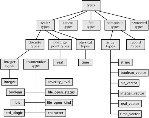
The scalar types are all those composed of individual values that are ordered. Integer and floating-point types are ordered on the number line. Physical types are ordered by the number of primary units in each value. Enumeration types are ordered by their declaration. The discrete types are those that represent discrete sets of values and comprise the integer types and enumeration types. Floating-point and physical types are not discrete, as they approximate a continuum of values.
In Section 2.2 we saw how to declare a type, which defines a set of values. Often a model contains objects that should only take on a restricted range of the complete set of values. We can represent such objects by declaring a subtype, which defines a restricted set of values from a base type. The condition that determines which values are in the subtype is called a constraint. Using a subtype declaration makes clear our intention about which values are valid and makes it possible to check that invalid values are not used. The simplified syntax rules for a subtype declaration are
   subtype_declaration ⇐ subtype identifier is subtype_indication;
   subtype_indication ⇐
     type_mark [ range simple_expression ( to | downto ) simple_expression ]
We will look at more advanced forms of subtype indications in later chapters. The subtype declaration defines the identifier as a subtype of the base type specified by the type mark, with the range constraint restricting the values for the subtype. The constraint is optional, which means that it is possible to have a subtype that includes all of the values of the base type.
Here is an example of a declaration that defines a subtype of integer:
subtype small_int is integer range –128 to 127;
Values of small_int are constrained to be within the range -128 to 127. If we declare some variables:
   variable deviation : small_int;
   variable adjustment : integer;
we can use them in calculations:
deviation := deviation + adjustment;
Note that in this case, we can mix the subtype and base type values in the addition to produce a value of type integer, but the result must be within the range -128 to 127 for the assignment to succeed. If it is not, an error will be signaled when the variable is assigned. All of the operations that are applicable to the base type can also be used on values of a subtype. The operations produce values of the base type rather than the subtype. However, the assignment operation will not assign a value to a variable of a subtype if the value does not meet the constraint.
Another point to note is that if a base type is a range of one direction (ascending or descending), and a subtype is specified with a range constraint of the opposite direction, it is the subtype specification that counts. For example, the predefined type integer is an ascending range. If we declare a subtype as
subtype bit_index is integer range 31 downto 0;
this subtype is a descending range.
The VHDL standard includes two predefined integer subtypes, defined as
   subtype natural is integer range 0 to highest_integer;
   subtype positive is integer range 1 to highest_integer;
Where the logic of a design indicates that a number should not be negative, it is good style to use one of these subtypes rather than the base type integer. In this way, we can detect any design errors that incorrectly cause negative numbers to be produced. There is also a predefined subtype of the physical type time, defined as
subtype delay_length is time range 0 fs to highest_time;
This subtype should be used wherever a non-negative time delay is required.
Sometimes it is not clear from the context what the type of a particular value is. In the case of overloaded enumeration literals, it may be necessary to specify explicitly which type is meant. We can do this using type qualification, which consists of writing the type name followed by a single quote character, then an expression enclosed in parentheses. For example, given the enumeration types
   type logic_level is (unknown, low, undriven, high);
   type system_state is (unknown, ready, busy);
we can distinguish between the common literal values by writing
logic_level'(unknown) system_state'(unknown)
Type qualification can also be used to narrow a value down to a particular subtype of a base type. For example, if we define a subtype of logic_level
subtype valid_level is logic_level range low to high;
we can explicitly specify a value of either the type or the subtype
logic_level'(high) valid_level'(high)
Of course, it is an error if the expression being qualified is not of the type specified.
VHDL-87, -93, and -2002
In these earlier versions of VHDL, if a type qualification specified a subtype, the value qualified had to be of that specific subtype. It was not sufficient for it just to be of the base type of the specified subtype. In VHDL-2008, the value is converted to be of the subtype. While there is no distinction in the case of scalar types, when we come to composite types, the distinction can be significant.
When we introduced the arithmetic operators in previous sections, we stated that the operands must be of the same type. This precludes mixing integer and floating-point values in arithmetic expressions. Where we need to do mixed arithmetic, we can use type conversions to convert between integer and floating-point values. The form of a type conversion is the name of the type we want to convert to, followed by a value in parentheses. For example, to convert between the types integer and real, we could write
real(123) integer(3.6)
Converting an integer to a floating-point value is simply a change in representation, although some loss of precision may occur. Converting from a floating-point value to an integer involves rounding to the nearest integer. Numeric type conversions are not the only conversion allowed. In general, we can convert between any closely related types. Other examples of closely related types are certain array types, discussed in Chapter 4.
One thing to watch out for is the distinction between type qualification and type conversion. The former simply states the type of a value, whereas the latter changes the value, possibly to a different type. One way to remember this distinction is to think of “quote for qualification.”
A type defines a set of values and a set of applicable operations. There is also a predefined set of attributes that are used to give information about the values included in the type. Attributes are written by following the type name with a quote mark ( ‘) and the attribute name. The value of an attribute can be used in calculations in a model. We now look at some of the attributes defined for the types we have discussed in this chapter.
First, there are a number of attributes that are applicable to all scalar types and provide information about the range of values in the type. If we let T stand for any scalar type or subtype, x stand for a value of that type and s stand for a string value, the attributes are
   T'left           first (leftmost) value in T
   T'right          last (rightmost) value in T
   T'low            least value in T
   T'high           greatest value in T
   T'ascending      true if T is an ascending range, false otherwise
   T'image(x)       a string representing the value of x
   T'value(s)       the value in T that is represented by s
The string produced by the ‘image attribute is a correctly formed literal according to the rules shown in Chapter 1. The strings allowed in the ‘value attribute must follow those rules and may include leading or trailing spaces. These two attributes are useful for input and output in a model, as we will see when we come to that topic.
To illustrate the attributes listed above, recall the following declarations from previous examples:
   type resistance is range 0 to 1E9
    units
      ohm;
      kohm = 1000 ohm;
      Mohm = 1000 kohm;
    end units resistance;
   type set_index_range is range 21 downto 11;
   type logic_level is (unknown, low, undriven, high);
For these types:
   resistance'left = 0 ohm
   resistance'right = 1E9 ohm
   resistance'low = 0 ohm
   resistance'high = 1E9 ohm
   resistance'ascending = true
   resistance'image(2 kohm) = "2000 ohm'
   resistance'value("5 Mohm") = 5_000_000 ohm

   set_index_range'left = 21
   set_index_range'right = 11
   set_index_range'low = 11
   set_index_range'high = 21
   set_index_range'ascending = false
   set_index_range'image(14) = "14"
   set_index_range'value("20") = 20

   logic_level'left = unknown
   logic_level'right = high
   logic_level'low = unknown
   logic_level'high = high
   logic_level'ascending = true
   logic_level'image(undriven) = "undriven"
   logic_level'value("Low") = low
Next, there are attributes that are applicable to just discrete and physical types. For any such type T, a value x of that type and an integer n, the attributes are
   T'pos(x)      position number of x in T
   T'val(n)      value in T at position n
   T'succ(x)     value in T at position one greater than that of x
   T'pred(x)     value in T at position one less than that of x
   T'leftof(x)   value in T at position one to the left of x
   T'rightof(x)  value in T at position one to the right of x
For enumeration types, the position numbers start at zero for the first element listed and increase by one for each element to the right. So, for the type logic_level shown above, some attribute values are
   logic_level'pos(unknown) = 0
   logic_level'val(3) = high
   logic_level'succ(unknown) = low
   logic_level'pred(undriven) = low
For integer types, the position number is the same as the integer value, but the type of the position number is a special anonymous type called universal integer. This is the same type as that of integer literals and, where necessary, is implicitly converted to any other declared integer type. For physical types, the position number is the integer number of base units in the physical value. For example:
time'pos(4 ns) = 4_000_000
since the base unit is fs.
We can use the ‘pos and ‘val attributes in combination to perform mixed-dimensional arithmetic with physical types, producing a result of the correct dimensionality. Suppose we define physical types to represent length and area, as follows:
   type length is range integer'low to integer'high
     units
       mm;
     end units length;

   type area is range integer'low to integer'high
     units
       square_mm;
     end units area;
and variables of these types:
   variable L1, L2 : length;
   variable A : area;
The restrictions on multiplying values of physical types prevents us from writing something like
A := L1 * L2; -- this is incorrectTo achieve the correct result, we can convert the length values to abstract integers using the ‘pos attribute, then convert the result of the multiplication to an area value using ‘val, as follows:
A := area'val( length'pos(L1) * length'pos(L2) );
Note that in this example, we do not need to include a scale factor in the multiplication, since the base unit of area is the square of the base unit of length.
For ascending ranges, T‘succ(x) and T‘rightof(x) produce the same value, and T‘pred(x) and T‘leftof(x) produce the same value. For descending ranges, T‘pred(x) and T‘rightof(x) produce the same value, and T‘succ(x) and T‘leftof(x) produce the same value. For all ranges, T‘succ(T‘high), T‘pred(T‘low), T‘rightof(T‘right) and T‘leftof(T‘left) cause an error to occur.
The last attribute we introduce here is T‘base. For any subtype T, this attribute produces the base type of T. The only context in which this attribute may be used is as the prefix of another attribute. For example, if we have the declarations
   type opcode is
     (nop, load, store, add, subtract, negate, branch, halt);
   subtype arith_op is opcode range add to negate;
then
   arith_op'base'left = nop
   arith_op'base'succ(negate) = branch
In Section 2.1 we showed how the value resulting from evaluation of an expression can be assigned to a variable. In this section, we summarize the rules governing expressions. We can think of an expression as being a formula that specifies how to compute a value. As such, it consists of primary values combined with operators and other operations. The precise syntax rules for writing expressions are shown in Appendix B. The primary values that can be used in expressions include
We have seen examples of these in this chapter and in Chapter 1. For reference, all of the predefined operators and the types they can be applied to are summarized in Table 2.2. We will discuss array operators in Chapter 4. The operators in this table are grouped by precedence, with “**”, abs, and the unary logical reduction operators having highest precedence and the binary logical operators lowest. In addition, the condition operator “??” can only be applied to a primary value at the outermost level of an expression. The precedence rules mean that if an expression contains a combination of operators, those with highest precedence are applied first. Parentheses can be used to alter the order of evaluation, or for clarity.
Table 2.2. VHDL operators in order of precedence, from most binding to least binding
Operator | Operation | Left operand type | Right operand type | Result type |
|---|---|---|---|---|
| exponentiation | integer or floating-point | integer | same as left operand |
| absolute value | numeric | same as operand | |
| logical negation |
| same as operand | |
| logical and reductionlogical or reductionnegated logical and reductionnegated logical or reductionexclusive or reductionnegated exclusive or reduction | 1-D array of | element type of operand | |
* | multiplication | integer or floating-pointphysical | same as left operand | same as operandssame as left operandsame as right operand |
/ | division | integer or floating-pointphysicalphysical | same as left operandinteger or realsame as left operand | same as operandssame as left operanduniversal integer |
| moduloremainder | integer or physical | same as left operand | same as operands |
+- | identitynegation | numeric | same as operand | |
+- | additionsubtraction | numeric | same as left operand | same as operands |
& | concatenation | 1-D array1-D arrayelement type of right operandelement type of result | same as left operandelement type of left operand1-D arrayelement type of result | same as operandssame as left operandsame as right operand1-D array |
| shift-left logicalshift-right logicalrotate leftrotate right |
| integer | same as left operand |
| shift-left arithmeticshift-right arithmetic |
| integer | same as left operand |
=/= | equalityinequality | any except file orprotected type | same as left operand |
|
<<=>>= | less thanless than or equal togreater thangreater than or equal to | scalar or 1-D array of any discrete type | same as left operand |
|
?=?/= | matching equalitymatching inequality |
| same as left operand |
|
?<?<=?>?>= | matching less thanmatching less than or equal tomatching greater thanmatching greater than or equal to |
| same as left operand |
|
| logical andlogical ornegated logical andnegated logical orexclusive ornegated exclusive or |
| same as left operand | same as operands |
?? | condition conversion |
|
|
In Section 2.2, we described the maximum and minimum operations for numeric types. These are examples of function operations that can form primary values in expressions. In fact, these operations are defined for all scalar types, as are the relational operators “<”, “<=”, “>”, and “>=”. For numeric types, the maximum and minimum operations compare the numeric values to determine the result. For enumeration types, the operations compare the position numbers. Thus, enumeration values declared earlier in the list of an enumeration type declaration are considered to be less than those declared later in the list. For example, in the character type, ‘A’ < ‘Z’, and the minimum of ‘c’ and ‘q’ is ‘c’.
Another function operation that can be applied to any scalar value is the to_string operation. It yields a character-string representation of the value that can be used in any place where we can use a string literal. For example:
   to_string(123)     = "123"
   to_string(456.78)  = "4.5678e+2"
   to_string(warning) = "warning"
For floating-point types, to_string represents the value using exponential notation, with the number of digits depending on the particular VHDL tool being used. There are, however, two alternate forms of to_string for floating-point values that give us more control over the formatting. First, we can specify that the value be represented with a given number of post-decimal digits rather than in exponential form. For example:
   to_string(456.78, 4) = "456.7800"
   to_string(456.78, 1) = "456.8"
Second, we can provide a format specification string of the same form as that used in the C printf function. For example:
   to_string(456.78, "%10.3f")  = "  456.780"
   to_string(456.78, "%-12.3E") = "4.568E+02   "
For physical types, to_string represents the value using the primary unit of the type. For example, given the declaration of type resistance on page 39:
to_string(2.2 kohm) = "2200 ohm"
The exception is the physical type time, for which to_string represents the value as a multiple of the resolution limit. So, for example, if the resolution limit for a simulation is set to ns:
to_string(29.5 us) = "29500 ns"
There is also an alternate form of to_string for time that allows us to control the unit used to represent the value. For example, even if the resolution limit is set to ns, we can represent a time value in microseconds as follows:
to_string(29500 ns, us) = "29.5 us"
The final predefined function operations on scalar types are the rising_edge and falling_edge operations, which can be applied to signals of type boolean, bit, or std_ulogic. These allow us to describe edge-triggered behavior in a natural manner. For example, we can write a process describing a D-flipflop as follows:
   signal clk, d, q : bit;
   ...
   dff : process is
   begin
     if rising_edge(clk) then
       q <= d;
     end if;
     wait on clk;
   end process dff;
For a boolean signal s, rising_edge(s) is true when s changes from false to true and false at other times (including when s changes from true to false and when s is not changing). Similarly, falling_edge(s) is true when s changes from true to false and false at other times. For a bit signal s, rising_edge(s) is true when s changes from ‘0’ to ‘1’ and false at other times; and falling_edge(s) is true when s changes from ‘1’ to ‘0’, and false at other times. Finally, for a std_ulogic signal s, rising_edge(s) is true when s changes from ‘0’ or ‘L’ to ‘1’ or ‘H’ and false at other times (including changes from or to ‘U’, ‘X’, ‘W’, ‘Z’, or ‘–’); and falling_edge(s) is true when s changes from ‘1’ or ‘H’ to ‘0’ or ‘L’ and false at other times.
VHDL-87, -93, and -2002
The unary logical operators (and, or, nand, nor, xor and xnor), the matching relational operators (“?=”, “?/=”, “?<”,“?<=”, “?>”, and “?>=”), the condition conversion operator (“??”), and the function operations maximum, minimum, to_string, rising_edge, and falling_edge are not provided in earlier versions of VHDL. Also, the mod and rem operators are not applicable to physical types in earlier versions.
[ | |
[ | |
[ | |
[ | |
[ signal a, b, c : std_ulogic; type state_type is (idle, req, ack); signal state : state_type; indicate whether each of the following expressions is legal as a Boolean condition, and if not, correct it:
| |
[ subtype pulse_range is time range 1 ms to 100 ms; subtype word_index is integer range 31 downto 0; what are the values of | |
[ type state is (off, standby, active1, active2); what are the values of state'pos(standby) state'val(2) state'succ(active2) state'pred(active1) state'leftof(off) state'rightof(off) | |
[ 2 * 3 + 6 / 4 3 + -4
"cat" & character'('0') true and x and not y or z
B"101110" sll 3 (B"100010" sra 2) & X"2C" | |
9. | [ |
10. | [ |
11. | [ |
12. | [ clock_gen : process is begin clk <= '1' wait for 10 ns; clk <= '0' wait for 10 ns; end process clock_gen; Use this as the basis for experiments to determine how your simulator behaves with different settings for the resolution limit. Try setting the resolution limit to 1 ns (the default for many simulators), 1 ps and 1 μs. |
13. | [ |