
10 Arrays
Init, Use, Destroy. Three procedure calls, six possible sequences, five of them wrong. I am quietly impressed that any nontrivial applications ever work.—Thomas L. Holaday
Because there’s no built-in array data type, there’s really no direct way to store or work with true arrays in Transact-SQL. There are a couple of alternatives that are fairly array-like, but since they really aren’t arrays in the 3GL sense of the word, they’re less than ideal.
The two most obvious ways to simulate an array in Transact-SQL are setting up a table that mimics an array (with columns simulating dimensions) and using a single column to store multiple values (with special indexing routines to flatten or compose the array elements). The first approach has the advantage of being more relational and extensible. Adding a dimension is as simple as adding a column. The second approach has the advantage of simplicity and intuitiveness. Having a column that stores multiple values is not far removed from having one that can store an array—it’s largely a question of semantics and syntax.
Note that arrays, by their very nature, violate the basic rules of normalization. For a table to be even first normal form compliant, it must be free of repeating values. Repeating values can take the form of multiple columns used to store instances of the same type of value or multiple values within a single column. These repeating values must be removed if a table is to be considered normalized. Storing arrays—even “virtual” arrays like the ones discussed in this chapter—is a form of denormalization that you should undertake only in special circumstances.
Storing arrays as large character strings is not a new concept. In fact, in the 1980s, the Advanced Revelation DBMS garnered quite a following through its support of “multivalued” columns—essentially string fields with multiple values and special routines to manipulate them. Even today, many DBMSs that support array columns store them internally as simple buffers and provide SQL extensions that insulate the developer from having to know or deal with this. Here’s a sample query that demonstrates the multivalued column approach in Transact-SQL:
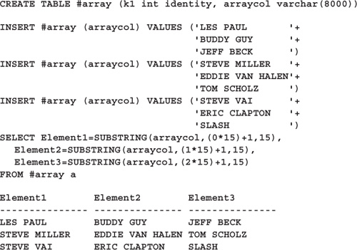
This technique stores multiple values in the work table’s arraycol column. These values emulate a single-dimensional array, which is the easiest type to work with using this approach. Multidimensional arrays are feasible as well, but they’re exponentially more complex to deal with. Rather than building multidimensional arrays into a single row, another way to accomplish the same thing is to spread the dimensions of the array over the entire table, with each record representing just one row in that array.
Note the use of varchar(8000) to define the array column. With the advent of SQL Server’s large character data types, we can now store a reasonably sized array using this approach. In the case of an array whose elements are fifteen bytes long, we can store up to 533 items in each array column, in each row. That’s plenty for most applications.
Also note that virtually any type of data can be stored in this type of virtual array, not just strings. Of course, anything stored in a character column must be converted to a string first, but that’s a minor concern. The only prerequisite is that each item must be uniformly sized, regardless of its original data type.
The INSERT statements used to populate the table are intentionally split over multiple lines to mimic filling an array. Though it’s unnecessary, you should consider doing this as well if you decide to use this approach. It’s more readable and also helps with keeping each element sized appropriately—an essential for the technique to work correctly.
Note the use of the expression (n*s)+1 to calculate each array element’s index. Here, n represents the element number (assuming a base of zero) you wish to access, and s represents the element size. Though it would be easier to code
SUBSTRING(arraycol,1,15)
using the expression establishes the relationship between the element you seek and the string stored in the varchar column. It makes accessing any element as trivial as supplying its array index.
This technique does not require that the number of elements be uniform between rows in the table. Here’s an example that shows how to implement “jagged” or unevenly sized arrays:
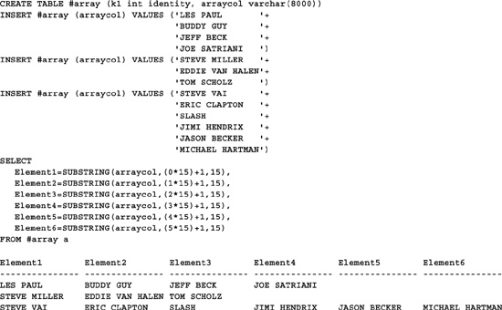
The only thing that’s really different here is the data. Since SUBSTRING() returns an empty string when passed an invalid starting point, we don’t need special handling for arrays with fewer than six elements.
The example above is limited to arrays with six or fewer elements. What if we want to support arrays of sixty elements? What if we need arrays with hundreds of elements? Are we forced to include a separate column in the result set for each one? The technique would be rather limited if we had to set up a separate result set column for every element. That would get cumbersome in a hurry. Here’s some code that demonstrates how to handle arrays of any size without coding static result set columns for each element:
DECLARE @arrayvar varchar(8000)
DECLARE @i int, @l int
DECLARE c CURSOR FOR SELECT arraycol FROM #array
OPEN c
FETCH c INTO @arrayvar
WHILE (@@FETCH_STATUS=0) BEGIN
SET @i=0
SET @l=DATALENGTH(@arrayvar)/15
WHILE (@i<@l) BEGIN
SELECT 'Guitarist'=SUBSTRING(@arrayvar,(@i*15)+1,15)
SET @i=@i+1
END
FETCH c INTO @arrayvar
END
CLOSE c
DEALLOCATE c
Guitarist
---------------
LES PAUL
Guitarist
---------------
BUDDY GUY
Guitarist
---------------
JEFF BECK
Guitarist
---------------
JOE SATRIANI
Guitarist
---------------
STEVE MILLER
Guitarist
---------------
EDDIE VAN HALEN
Guitarist
---------------
TOM SCHOLZ
Guitarist
---------------
STEVE VAI
Guitarist
---------------
ERIC CLAPTON
Guitarist
---------------
SLASH
Guitarist
---------------
JIMI HENDRIX
Guitarist
---------------
JASON BECKER
Guitarist
---------------
MICHAEL HARTMAN
This code opens a cursor on the work table, then iterates through the array in each row. It uses the DATALENGTH() function to determine the length of each array and a loop to SELECT each element from the array using the indexing expression introduced in the previous query.
Though this technique is flexible in that it allows us to process as many array elements as we want with a minimum of code, it suffers from one fundamental flaw: It returns multiple result sets. Many front ends don’t know how to handle multiple result sets and will balk at query output such as this. There are a couple of ways around this. Here’s one approach:
CREATE TABLE #results (Guitarist varchar(15))
DECLARE @arrayvar varchar(8000)
DECLARE @i int, @l int
DECLARE c CURSOR FOR SELECT arraycol FROM #array
OPEN c
FETCH c INTO @arrayvar
WHILE (@@FETCH_STATUS=0) BEGIN
SET @i=0
SET @l=DATALENGTH(@arrayvar)/15
WHILE (@i<@l) BEGIN
INSERT #results SELECT SUBSTRING(@arrayvar,(@i*15)+1,15)
SET @i=@i+1
END
FETCH c INTO @arrayvar
END
CLOSE c
DEALLOCATE c
SELECT * FROM #results
DROP TABLE #results
Guitarist
---------------
LES PAUL
BUDDY GUY
JEFF BECK
JOE SATRIANI
STEVE MILLER
EDDIE VAN HALEN
TOM SCHOLZ
STEVE VAI
ERIC CLAPTON
SLASH
JIMI HENDRIX
JASON BECKER
MICHAEL HARTMAN
Here, we use a temporary table to store each array element as it’s processed by the query. Once processing completes, the contents of the table are returned as a single result set and the temporary table is dropped. A variation on this would be to move the code to a stored procedure and return a pointer to the cursor via an output parameter. Then the caller could process the array at its convenience.
Another, though slightly more limited, way to process the array is to generate a SELECT statement as the array is processed and execute it afterward. Here’s an example:
DECLARE @arrayvar varchar(8000), @select_stmnt varchar(8000)
DECLARE @k int, @i int, @l int, @c int
DECLARE c CURSOR FOR SELECT * FROM #array
SET @select_stmnt=’SELECT '
SET @c=0
OPEN c
FETCH c INTO @k, @arrayvar
WHILE (@@FETCH_STATUS=0) BEGIN
SET @i=0
SET @l=DATALENGTH(@arrayvar)/15
WHILE (@i<@l) BEGIN
SELECT @select_stmnt=@select_stmnt+'Guitarist'+CAST(@c as
varchar)+'='+QUOTENAME(RTRIM(SUBSTRING(@arrayvar,(@i*15)+1,15)),'"')+','
SET @i=@i+1
SET @c=@c+1
END
FETCH c INTO @k, @arrayvar
END
CLOSE c
DEALLOCATE c
SELECT @select_stmnt=LEFT(@select_stmnt,DATALENGTH(@select_stmnt)-1)
EXEC(@select_stmnt)
(Results abridged)
Guitarist0 Guitarist1 Guitarist2 Guitarist3 Guitarist4 Guitarist5
---------- ------------------ --------------- ----------------- -------------------- ---------------
LES PAUL BUDDY GUY JEFF BECK JOE SATRIANI STEVE MILLER EDDIE VAN HALEN
Note the use of the QUOTENAME() function to surround each array value with quotes so that it can be returned by the SELECT statement. The default quote delimiters are '[' and ']' but, as the example shows, you can specify others.
This routine is more limited than the temporary table solution because it’s restricted by the maximum size of varchar. That is, since the SELECT statement that we build is stored in a variable of type varchar, it can’t exceed 8000 bytes. While the other techniques allot 8000 bytes for each row’s array, this one limits the sum length of the arrays in all records to just 8000 bytes. Given that this string must also store a column name for each element (most front ends have trouble processing unnamed columns), this is a significant limitation.
Nevertheless, the fact that this approach builds SQL that it then executes is interesting in and of itself. You can probably think of other applications for this technique such as variably sized cross-tabs, run and sequence flattening, and so on.
One inherent weakness of storing arrays as strings is revealed when we attempt to make modifications to element values. Unless you’re making the most basic kind of change, updating either a single value or an entire dimension is not a straightforward process. Clearing the array in a given row is simple—we just do something like this:
UPDATE #array SET arraycol = '' WHERE k1=1
If you think of the array in each record as a row in a larger array (which spans the entire table), you can think of this as clearing a single row.
What if we wanted to clear just the second element in each record’s array? We’d need something like this:
UPDATE #array
SET arraycol =
LEFT(arraycol,1*15)+SPACE(1*15)+RIGHT(arraycol,DATALENGTH(arraycol)-(2*15))
(Results abridged)

This involves a few somewhat abstruse computations that depend on the element size to work correctly. As with the earlier queries, this code multiplies an array index by the element size in order to access the array. Though it’s certainly more compact to use SPACE(15) rather than SPACE(1*15), using the expression is more flexible in that it’s easily reusable with other elements.
Note that we could use this technique to set the value of a particular dimension rather than simply clearing it. For example, to fill the third element in each row’s array with a specific value, we would use code like this:
UPDATE #array
SET arraycol =
LEFT(arraycol,(2*15))+'MUDDY WATERS '+RIGHT(arraycol,DATALENGTH(arraycol)-(3*15))
To limit the change to a particular record, include a WHERE clause that restricts the UPDATE, like this:
UPDATE #array
SET arraycol =
LEFT(arraycol,(3*15))+'MUDDY WATERS '+
RIGHT(arraycol,CASE WHEN (DATALENGTH(arraycol)-(4*15))<0 THEN 0 ELSE
DATALENGTH(arraycol)-(4*15) END)
WHERE k1=2
As you can see, things can get pretty convoluted considering all we want to do is change an array element. Naturally, things would be much simpler if Transact-SQL supported arrays directly.
Implementing a virtual array using a simple table is also a viable alternative to native array support. This technique uses one or more columns as array indexes. If the array is single-dimensional, there’s just one index column. If it’s multidimensional, there may be several. Here’s an example:
CREATE TABLE #array (k1 int identity (0,1), guitarist varchar(15))
INSERT #array (guitarist) VALUES('LES PAUL'),
INSERT #array (guitarist) VALUES('BUDDY GUY'),
INSERT #array (guitarist) VALUES('JEFF BECK'),
INSERT #array (guitarist) VALUES('JOE SATRIANI'),
INSERT #array (guitarist) VALUES(’STEVE MILLER'),
INSERT #array (guitarist) VALUES('EDDIE VAN HALEN'),
INSERT #array (guitarist) VALUES(’TOM SCHOLZ'),
INSERT #array (guitarist) VALUES(’STEVE VAI'),
INSERT #array (guitarist) VALUES('ERIC CLAPTON'),
INSERT #array (guitarist) VALUES(’SLASH'),
INSERT #array (guitarist) VALUES('JIMI HENDRIX'),
INSERT #array (guitarist) VALUES('JASON BECKER'),
INSERT #array (guitarist) VALUES('MICHAEL HARTMAN'),
-- To set the third element in the array
UPDATE #array
SET guitarist='JOHN GMUENDER'
WHERE k1=2
SELECT guitarist
FROM #array
guitarist
---------------
LES PAUL
BUDDY GUY
JOHN GMUENDER
JOE SATRIANI
STEVE MILLER
EDDIE VAN HALEN
TOM SCHOLZ
STEVE VAI
ERIC CLAPTON
SLASH
JIMI HENDRIX
JASON BECKER
MICHAEL HARTMAN
This code illustrates a simple way to emulate a single-dimensional array using a table. Note the use of a seed value for the identity column in order to construct a zero-based array, as we did in the string array examples. Transact-SQL requires that you also specify an increment value whenever you specify a seed value, so we specified an increment of one.
This code changes the value of the third element (which has an index value of two). Removing the WHERE clause would allow the entire virtual array to be set or cleared.
Unlike the varchar array technique, sorting a virtual table array is as simple as supplying an ORDER BY clause. Deleting elements is simple, too—all you need is a DELETE statement qualified by a WHERE clause. Inserting a new element (as opposed to appending one) is more difficult since we’re using an identity column as the array index. However, it’s still doable—either via SET IDENTITY_INSERT or by changing the index column to a nonidentity type.
Adding a dimension is as straightforward as adding a column. Here’s an example:
CREATE TABLE #array (band int, single int, title varchar(50))
INSERT #array VALUES(0,0,'LITTLE BIT O'' LOVE'),
INSERT #array VALUES(0,1,'FIRE AND WATER'),
INSERT #array VALUES(0,2,’THE FARMER HAD A DAUGHTER'),
INSERT #array VALUES(0,3,'ALL RIGHT NOW'),
INSERT #array VALUES(1,0,'BAD COMPANY'),
INSERT #array VALUES(1,1,’SHOOTING STAR'),
INSERT #array VALUES(1,2,'FEEL LIKE MAKIN'' LOVE'),
INSERT #array VALUES(1,3,'ROCK AND ROLL FANTASY'),
INSERT #array VALUES(2,0,’SATISFACTION GUARANTEED'),
INSERT #array VALUES(2,1,'RADIOACTIVE'),
INSERT #array VALUES(2,2,'MONEY CAN'’T BUY'),
INSERT #array VALUES(2,3,’TOGETHER'),
INSERT #array VALUES(3,0,'GOOD MORNING LITTLE SCHOOLGIRL'),
INSERT #array VALUES(3,1,'HOOCHIE-COOCHIE MAN'),
INSERT #array VALUES(3,2,'MUDDY WATER BLUES'),
INSERT #array VALUES(3,3,’THE HUNTER'),
-- To set the third element in the fourth row of the array
UPDATE #array
SET title='BORN UNDER A BAD SIGN'
WHERE band=3 AND single=2
SELECT title
FROM #array
title
--------------------------------------------------
LITTLE BIT O' LOVE
FIRE AND WATER
THE FARMER HAD A DAUGHTER
ALL RIGHT NOW
BAD COMPANY
SHOOTING STAR
FEEL LIKE MAKIN' LOVE
ROCK AND ROLL FANTASY
SATISFACTION GUARANTEED
RADIOACTIVE
MONEY CAN’T BUY
TOGETHER
GOOD MORNING LITTLE SCHOOLGIRL
HOOCHIE-COOCHIE MAN
BORN UNDER A BAD SIGN
THE HUNTER
This code sets up a two-dimensional array, then changes the third element in its fourth row. Because its indexes are simple integer columns, the SQL necessary to manipulate the array is much more intuitive. For example, clearing a given dimension in the array is trivial:
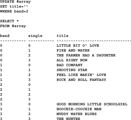
This code uses a simple UPDATE statement qualified by a WHERE clause to clear the array’s third dimension.
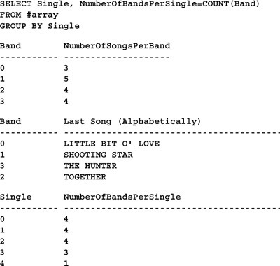
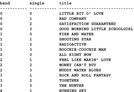
Another nifty feature of this approach is that row and column totals are easy to produce using basic aggregate functions and the GROUP BY clause. Here’s a query that performs a variety of aggregations using the array’s indexes as grouping columns:
CREATE TABLE #array (band int, single int, title varchar(50))
INSERT #array VALUES(0,0,'LITTLE BIT O'' LOVE'),
INSERT #array VALUES(0,1,'FIRE AND WATER'),
INSERT #array VALUES(0,2,'ALL RIGHT NOW'),
INSERT #array VALUES(1,0,'BAD COMPANY'),
INSERT #array VALUES(1,1,’SHOOTING STAR'),
INSERT #array VALUES(1,2,'FEEL LIKE MAKIN'' LOVE'),
INSERT #array VALUES(1,3,'ROCK AND ROLL FANTASY'),
INSERT #array VALUES(1,4,'BURNING SKY'),
INSERT #array VALUES(2,0,’SATISFACTION GUARANTEED'),
INSERT #array VALUES(2,1,'RADIOACTIVE'),
INSERT #array VALUES(2,2,'MONEY CAN'’T BUY'),
INSERT #array VALUES(2,3,’TOGETHER'),
INSERT #array VALUES(3,0,'GOOD MORNING LITTLE SCHOOLGIRL'),
INSERT #array VALUES(3,1,'HOOCHIE-COOCHIE MAN'),
INSERT #array VALUES(3,2,'MUDDY WATER BLUES'),
INSERT #array VALUES(3,3,’THE HUNTER'),
SELECT Band, NumberOfSongsPerBand=COUNT(single)
FROM #array
GROUP BY Band
SELECT Band, "Last Song (Alphabetically)"=MAX(title)
FROM #array
GROUP BY Band
ORDER BY 2
Keep in mind that the index columns used with this approach can be data types other than integers since we access them via the WHERE clause. Datetime types, GUIDs, and bit types are popular indexes as well. Also, these indexes can be accessed via more complex expressions than the diminutive “=i” where i is an array index. The LIKE, BETWEEN, IN, and EXISTS predicates, as well as subqueries, can also be used to traverse the array.
Swapping array dimensions is also relatively trivial with this approach. For example, assume we have a two-dimensional array, and we want to swap its rows and columns. How would we do it? With the varchar array approach, this could get quite involved. However, it’s fairly straightforward using the table array approach and a feature of the UPDATE statement. Here’s the code:

Since Transact-SQL is processed left to right, we’re able to set @i to store the value of band so that we may swap band and single. The ability to set a local variable via UPDATE was originally intended as a performance enhancement to shorten the time locks were held. It was designed to combine the functionality of performing an UPDATE, then immediately SELECTing a value from the same table into a local variable for further processing. In our case, we’re using this feature, along with Transact-SQL’s left-to-right execution, to swap one column with another.
It’s possible that Transact-SQL’s ability to reuse variables set by an UPDATE within the UPDATE itself might change someday since it’s not specifically documented. As with all undocumented features, you should use it only when necessary and with due caution. It might not be supported in a future release, so be wary of becoming too dependent upon it.
Note that if you only want to swap the dimensions in the result set (rather than changing the array itself), that’s easy enough to do:
We get the same results as the previous query, but the array itself remains unmodified. A VIEW object is ideal in this situation if you need to swap an array’s dimensions on a regular basis.
There are a couple of nifty ways to ensure the veracity of the array index values you store. One is to create unique constraints on them. You can do this via PRIMARY KEY or UNIQUE KEY constraints on the appropriate columns. For example, we might modify the CREATE TABLE statement above like so:
CREATE TABLE #array (band int, single int, title varchar(50)
PRIMARY KEY (band, single))
This ensures that no duplicate indexes are allowed into the table, which is what you want. It also creates an index over the array indexes—which will probably benefit performance.
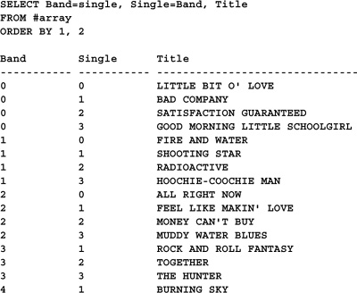
Many of the techniques that were used to reshape or flatten the varchar array work with table arrays as well. The most flexible of those presented is the technique that reshapes the array by populating a temporary table with values. However, table arrays give us another option that requires far less code and is much easier to follow:

This technique uses an aggregate to “hide” the selection of the title column for each band so that it can use GROUP BY to flatten the result set. It groups on the single column because single provides the type of unique identifier we need to coalesce the array elements. To understand this, it’s instructive to view what the result set would look like without the MAX()/ GROUP BY combo:
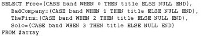

As the query traverses the table, it can fill only one column of our flattened array (actually just a simple cross-tab) at a time. Each column’s CASE expression establishes that. This means that for each row in the initial result set, every column will be NULL except one. This is where the MAX()/GROUP BY duo comes to the rescue. Grouping on single allows us to coalesce the values in each column so that these extraneous NULLs are removed. Using MAX() allows us to select each column while grouping (all nongrouping columns in the SELECT list must either be aggregates or constants when GROUP BY is present). Note that MIN() would have worked equally well. All we really need is an aggregate that can return the title column—the aggregate merely serves to support the use of GROUP BY—which is the opposite of how we usually think of the aggregate–GROUP BY relationship. Since MIN() and MAX() are the only two aggregates capable of returning character fields, we’re limited to using one of them.
It’s sometimes desirable to compare two arrays or two subsets of the same array with one another. This can be tricky because comparing arrays involves ordering the elements, whereas comparing plain sets does not. Here’s a modification of the previous code sample that checks elements of the table array against one another for equality:
CREATE TABLE #array (band int, single int, title varchar(30))
INSERT #array VALUES(0,0,'LITTLE BIT O'' LOVE'),
INSERT #array VALUES(0,1,'FIRE AND WATER'),
INSERT #array VALUES(0,2,'ALL RIGHT NOW'),
INSERT #array VALUES(0,3,’THE HUNTER'),
INSERT #array VALUES(1,0,'BAD COMPANY'),
INSERT #array VALUES(1,1,’SHOOTING STAR'),
INSERT #array VALUES(1,2,'FEEL LIKE MAKIN'' LOVE'),
INSERT #array VALUES(1,3,'ROCK AND ROLL FANTASY'),
INSERT #array VALUES(1,4,'BURNING SKY'),
INSERT #array VALUES(2,0,’SATISFACTION GUARANTEED'),
INSERT #array VALUES(2,1,'RADIOACTIVE'),
INSERT #array VALUES(2,2,'MONEY CAN'’T BUY'),
INSERT #array VALUES(2,3,’TOGETHER'),
INSERT #array VALUES(3,0,'GOOD MORNING LITTLE SCHOOLGIRL'),
INSERT #array VALUES(3,1,'HOOCHIE-COOCHIE MAN'),
INSERT #array VALUES(3,2,'MUDDY WATER BLUES'),
INSERT #array VALUES(3,3,’THE HUNTER'),
SELECT * FROM
(SELECT Free=MAX(CASE band WHEN 0 THEN title ELSE NULL END),
BadCompany=MAX(CASE band WHEN 1 THEN title ELSE NULL END),
TheFirm=MAX(CASE band WHEN 2 THEN title ELSE NULL END),
Solo=MAX(CASE band WHEN 3 THEN title ELSE NULL END)
FROM #array
GROUP BY single) a
WHERE Free=BadCompany
OR Free=TheFirm
OR Free=Solo
OR BadCompany=TheFirm
OR BadCompany=Solo
OR TheFirm=Solo
Free BadCompany TheFirm Solo
------------------ ------------------------------------------ --------------------- -----------------
THE HUNTER ROCK AND ROLL FANTASY TOGETHER THE HUNTER
This technique turns the earlier array flattening query into a derived table, which it then qualifies with a WHERE clause. (As mentioned in Chapter 7, you can think of a derived table as an implicit or inline VIEW.) It then returns all rows where the title of one band’s single is identical to that of another.
One problem with this approach is that it returns data we don’t need. The entries in the middle two columns are extraneous—all we really care about is that bands zero and three have singles with the same title. This could mean that one plagiarized the other, that the songwriters for one of the bands weren’t terribly original, or, perhaps, that the same lead singer sang for both.
Efficiency is another problem with this technique. The derived table selects every row in the #array table before handing it back to the outer query to pare down. Though the query optimizer will look at combining the two queries into one, the way that CASE is used here would probably confuse it. It would likely be more efficient to filter the rows returned as they’re selected rather than afterward. Here’s a code refinement that does that:
SELECT
Free=MAX(CASE a.band WHEN 0 THEN a.title ELSE NULL END),
BadCompany=MAX(CASE a.band WHEN 1 THEN a.title ELSE NULL END),
TheFirm=MAX(CASE a.band WHEN 2 THEN a.title ELSE NULL END),
Solo=MAX(CASE a.band WHEN 3 THEN a.title ELSE NULL END)
FROM #array a LEFT JOIN #array b ON (a.title=b.title)
WHERE NOT (a.band=b.band AND a.single=b.single)
GROUP BY a.single
Free BadCompany TheFirm Solo
------------------ --------------------- --------------------- -----------------
THE HUNTER NULL NULL THE HUNTER
The technique joins the array table with itself to locate duplicate elements. The query’s WHERE clause ensures that it doesn’t make the mistake of matching an element with itself. Since this approach filters the rows it returns as it processes them, it should be more efficient than the derived table approach. However, the introduction of a self-join may cancel out any performance gains achieved. Whether this technique is more efficient than the first one in a particular situation depends on the exact circumstances and data involved.
Note that this approach has the side effect of removing the extraneous values from the middle columns. Doing that with the derived table approach would be much more involved since it would basically amount to encoding the search criteria in two places: in the WHERE clause as well as in the SELECT list (via CASE expressions).
Since Transact-SQL doesn’t directly support arrays, they must be simulated using other constructs. The two most popular means of emulating arrays are to store them as large character fields and to set up table columns that mimic array dimensions. Using large strings for arrays is practical for single-dimensional constructs, but the table column approach is better for multidimensional arrays. Whatever type of faux array you elect to use, keep in mind that storing repeating values in a table row is a form a denormalization. Be sure that’s what you intend before you begin redesigning your database.
In this chapter, you learned to manipulate both types of pseudoarrays. You learned to add elements, to delete them, and to add and clear whole dimensions. You learned how to flatten simulated arrays into cross-tabs and to return array elements as result sets.