
6 The Mighty SELECT Statement
The fantasy element that explains the appeal of dungeon-clearing games to many programmers is neither the fire-breathing monsters nor the milky-skinned, semi-clad sirens; it is the experience of carrying out a task from start to finish without user requirements changing.—Thomas L. Holaday
As I said in Chapter 1, the SELECT statement is the workhorse of the Transact-SQL language. It does everything from assign variables to return result sets to create tables. Across all versions of SQL, SELECT is the Ginsu knife of the language. There was even a time when it was used to clear certain server error conditions in Sybase’s version of SQL Server (using a function called LCT_ADMIN()).
While it’s handy to be able to perform 75% of your work using a single tool, that tool has to be complex in order to offer all that functionality. A tool with so many features can be a bit unwieldy—you have to be careful lest you take off a finger.
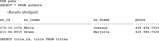
As was also pointed out in Chapter 1, SELECT statements need not be complex. Here are a few simple ones to prime the discussion:
In addition to garden-variety fields, you can specify functions, computations, and derived fields in the column list of a SELECT statement (commonly referred to as its “SELECT list”). Here are some examples:

You can include parameter-less functions like PI() and functions that require parameters like CAST(). You can use expressions that reference fields and expressions that don’t. You can perform basic computations in the SELECT list and can include subqueries that return single values. Here’s an example:

A derived column consists of a subquery that returns a single value. This subquery can be related to the outer query (correlated) or unrelated, but it must return a result set that is exactly one column by one row in size. We’ll cover correlated subqueries in more detail in a moment.
I’ve built the query using a derived field for illustration purposes only. It would be better written using a join, like so:
SELECT pub_name, COUNT(t.title_id) AS NumPublished
FROM publishers p LEFT JOIN titles t ON (p.pub_id = t.pub_id)
GROUP BY pub_name
This is frequently the case with subqueries—very often they can be restated as joins. These joins are sometimes more efficient because they avoid executing the secondary query for every row in the main table.
Prior to SQL Server 7.0, restricting the number of rows returned by a query required the use of the SET ROWCOUNT command. SET ROWCOUNT is still available, but there’s now a better way. SELECT TOP n [PERCENT] [WITH TIES] where n is the number or percentage of rows you wish to return is an efficient way to truncate query results. Here’s an example:

As you would expect, including the optional PERCENT keyword limits the rows returned to a percentage of the total number of rows.
Add the WITH TIES clause if you want to include ties—duplicate values—in the result set. Unless you’re merely trimming the result set to a particular size, TOP n logically implies ORDER BY. Although ORDER BY is optional with basic TOP n, the WITH TIES option requires it so that ties can be logically resolved. Here’s an example:

Even though TOP 4 is specified, five rows are returned because there’s a tie at position four. Note that this special tie handling works only for ties that occur at the end of the result set. That is, using the TOP 4 example, a tie at positions two and three will not cause more than four rows to be returned—only a tie at position four has this effect. This is counterintuitive and means that the following queries return the same result set as the TOP 4 query:
SELECT TOP 5 t.title, SUM(s.qty) AS TotalSales
FROM sales s JOIN titles t ON (s.title_id=t.title_id)
GROUP BY t.title
ORDER BY TotalSales DESC
and
SELECT TOP 5 WITH TIES t.title, SUM(s.qty) AS TotalSales
FROM sales s JOIN titles t ON (s.title_id=t.title_id)
GROUP BY t.title
ORDER BY TotalSales DESC
Another deficiency in TOP n is the fact that it can’t return grouped top segments in conjunction with a query’s GROUP BY clause. This means that a query like the one below can’t be modified to return the top store in each state using TOP n:

Though the syntax is supported, it doesn’t do what we might like:

As you can see, this query returns just one row. “TOP n” refers to the result set, not the rows in the original table or the groups into which they’ve been categorized. See the “Derived Tables” section below for an alternative to TOP n that returns grouped top subsets.
Besides direct references to tables and views, you can also construct logical tables on the fly in the FROM clause of a SELECT statement. These are called derived tables. A derived table is a subquery that’s used in place of a table or view. It can be queried and joined just like any other table or view. Here’s a very basic example:

The derived table in this query is constructed via the SELECT * FROM authors syntax. Any valid query could be inserted here and can contain derived tables of its own. Notice the inclusion of a table alias. This is a requirement of Transact-SQL derived tables—you must include it regardless of whether the query references other objects.
Since Transact-SQL supports nontabular SELECT statements, you can also use derived tables to construct logical tables from scratch without referencing any other database objects. Here’s an example:
SELECT *
FROM
(SELECT ’flyweight’ AS WeightClass, 0 AS LowBound, 112 AS HighBound
UNION ALL
SELECT ’bantamweight’ AS WeightClass, 113 AS LowerBound, 118 AS HighBound
UNION ALL
SELECT ’featherweight’ AS WeightClass, 119 AS LowerBound, 126 AS HighBound
UNION ALL
SELECT ’lightweight’ AS WeightClass, 127 AS LowerBound, 135 AS HighBound
UNION ALL
SELECT ’welterweight’ AS WeightClass, 136 AS LowerBound, 147 AS HighBound
UNION ALL
SELECT ’middleweight’ AS WeightClass, 148 AS LowerBound, 160 AS HighBound
UNION ALL
SELECT ’light heavyweight’ AS WeightClass, 161 AS LowerBound, 175 AS HighBound
UNION ALL
SELECT ’heavyweight’ AS WeightClass, 195 AS LowerBound, 1000 AS HighBound) W
ORDER BY W.LowBound

Here, we “construct” a derived table containing three columns and eight rows. Each SELECT represents a single row in this virtual table. The rows in the table are glued together using a series of UNIONs.
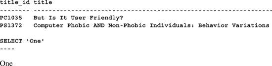
The table doesn’t actually exist anywhere—it’s a logical construct only. You can think of a derived table as a temporary VIEW object—it exists for the duration of the query then goes away quietly afterward. That a SELECT statement can be treated as a table is sensible given that, by definition, the result of a SQL query is itself a table—the result table. Here’s a query that joins a regular table with a derived table:
SELECT B.Name, B.Weight, W.WeightClass
FROM #boxers B,
(SELECT ’flyweight’ AS WeightClass, 0 AS LowBound, 112 AS HighBound
UNION ALL
SELECT ’bantamweight’ AS WeightClass, 113 AS LowerBound, 118 AS HighBound
UNION ALL
SELECT ’featherweight’ AS WeightClass, 119 AS LowerBound, 126 AS HighBound
UNION ALL
SELECT ’lightweight’ AS WeightClass, 127 AS LowerBound, 135 AS HighBound
UNION ALL
SELECT ’welterweight’ AS WeightClass, 136 AS LowerBound, 147 AS HighBound
UNION ALL
SELECT ’middleweight’ AS WeightClass, 148 AS LowerBound, 160 AS HighBound
UNION ALL
SELECT ’light heavyweight’ AS WeightClass, 161 AS LowerBound, 175 AS HighBound
UNION ALL
SELECT ’heavyweight’ AS WeightClass, 195 AS LowerBound, 1000 AS HighBound) W
WHERE B.Weight BETWEEN W.LowBound and W.HighBound
ORDER BY W.LowBound

This query first constructs a table containing a list of fictional boxers and each boxer’s fighting weight (our “regular” table). Next, it joins this table with the derived table introduced in the previous example to partition the list of boxers by weight class. Note that one of the boxers is omitted from the result because he doesn’t fall into any of the weight classes established by the derived table.
Of course, this query could have been greatly simplified using CASE statements, but the point of the exercise was to show the power of derived tables. Here, we “created” a multirow table via UNION and some simple SELECTs without requiring a real table.
This example illustrates some of the unique abilities of derived tables. Here’s an example that illustrates their necessity:

This query returns the store with the top sales in each state. As pointed out in the discussion of SELECT TOP n, it accomplishes what the TOP n extension is unable to—it returns a grouped top n result set.
In this case, a derived table is required in order to materialize the sales for each store without resorting to a VIEW object. Again, derived tables function much like inline views. Once each store’s sales have been aggregated from the sales table, the derived table is joined with itself using its state column to determine the number of other stores within each store’s home state that have fewer sales than it does. (Actually, we perform the inverse of this in order to give stores with more sales lower numbers, i.e., higher rankings.) This number is used to rank each store against the others in its state. The HAVING clause then uses this ranking to filter out all but the top store in each state. You could easily change the constant in the HAVING clause to include the top two stores, the top three, and so forth. The query is straightforward enough but was worth delving into in order to understand better the role derived tables play in real queries.
Of course, it would be more efficient to construct a static view to aggregate the sales for each store in advance. The query itself would be shorter and the optimizer would be more likely to be able to reuse the query plan it generates to service each aggregation:
CREATE VIEW SalesByState AS
SELECT s.stor_id, SUM(s.qty) AS TotalSales, t.state
FROM sales s JOIN stores t ON (s.stor_id=t.stor_id)
GROUP BY t.state, s.stor_id
SELECT s.state, st.stor_name,s.totalsales,Rank=COUNT(*)
FROM SalesByState s JOIN SalesByState t ON (s.state=t.state)
JOIN stores st ON (s.stor_id=st.stor_id)
WHERE s.totalsales <= t.totalsales
GROUP BY s.state,st.stor_name,s.totalsales
HAVING COUNT(*) <=1
ORDER BY s.state, rank
Nevertheless, there are situations where constructing a view in advance isn’t an option. If that’s the case, a derived table may be your best option.
Chapter 1 covers the different types of joins supported by Transact-SQL in some depth, so here I’ll focus on join nuances not covered there. Review Chapter 1 if you’re unsure of how joins work or need a refresher on join basics.
The ordering of the clauses in an inner join doesn’t affect the result set. If A=B, then certainly B=A. Inner join clauses are associative. That’s not true for outer joins. The order in which tables are joined directly affects which rows are included in the result set and which values they have. That’s why using the ANSI outer join syntax is so important—the legacy syntax can generate erroneous or ambiguous result sets because specifying join conditions in the WHERE clause precludes specifically ordering them.
To understand fully the effect join order has on OUTER JOINs, let’s explore the effect it has on the result set a query generates. Here’s a query that totals items in the Orders table of the Northwind sample database:
SELECT SUM(d.UnitPrice*d.Quantity) AS TotalOrdered
FROM Orders o LEFT OUTER JOIN [Order Details] d ON (o.OrderID+10=d.OrderID)
LEFT OUTER JOIN Products p ON (d.ProductID=p.ProductID)
TotalOrdered
---------------------
1339743.1900
I’ve intentionally introduced join condition failures into the query by incrementing o.OrderId by ten so that we can observe the effects of clause ordering and join failures on the result set. Now let’s reorder the tables in the FROM clause and compute the same aggregate:
SELECT SUM(d.UnitPrice * d.Quantity) AS TotalOrdered
FROM [Order Details] d LEFT OUTER JOIN Products p ON (d.ProductID=p.ProductID)
LEFT OUTER JOIN Orders o ON (o.OrderID+10=d.OrderID)
TotalOrdered
---------------------
1354458.5900
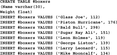
See the discrepancy? The total changes based on the order of the tables. Why? Because the first query introduces mismatches between the Orders and Order Details tables before the Unit-Price and Quantity columns are totaled; the second query does so afterward. In the case of the second query, we get a total of all items listed in the Order Details table regardless of whether there’s a match between it and the Orders table; in the first query, we don’t. To understand this better, consider the data on which the two totals are based:
I’ve included a WHERE clause to pare the result set down to just those rows affected by the intentional join mismatch. Since we increment OrderNo by ten and the order numbers are sequential, ten of the OrderNo values in Orders fail to find matches in the Order Details table and, consequently, have NULL UnitPrice and Quantity fields. Here’s a snapshot of the underlying data for the second query (again with a restrictive WHERE clause):
SELECT o.OrderDate, d.UnitPrice, d.Quantity
FROM [Order Details] d LEFT OUTER JOIN Products p ON (d.ProductID=p.ProductID)
LEFT OUTER JOIN Orders o ON (o.OrderID+10=d.OrderID)
WHERE o.OrderDate IS NULL
OR d.UnitPrice IS NULL

Notice that this set is much longer—nineteen rows longer, to be exact. Why? Because twenty-nine rows were omitted from the result set of the first query due to the join mismatch, though this wasn’t immediately obvious. For each broken order number link, a given number of Order Detail rows were omitted because there was a one-to-many relationship between the Orders and Order Details tables. This, of course, skewed the total reported by the query.
So the moral of the story is this: Be careful with outer join ordering, especially when the possibility of join mismatches exists.
By definition, a predicate is an expression that returns TRUE or NOT TRUE (I’m not using “FALSE” because of the issues related to three-valued logic—sometimes we don’t know whether an expression is FALSE, all we know is that it is not certainly TRUE).
Predicates are usually found in a query’s WHERE or HAVING clauses, though they can be located elsewhere (e.g., in CASE expressions). Predicates can be simple logical expressions or can be composed of functions that return TRUE or NOT TRUE. Though technically any function can be included in a predicate expression, Transact-SQL defines a number of predicate functions that are specifically geared toward filtering queries and result sets. The sections that follow detail each of them.
The BETWEEN predicate is probably the most often used of the Transact-SQL predicates. It indicates whether a given value falls between two other values, inclusively. Here’s an example:

BETWEEN works with scalar ranges, so it can handle dates, numerics, and other scalar data types. It combines what would normally require two terms in the WHERE clause: a greater-than-or-equal-to expression, followed by a less-than-or-equal-to expression. WHERE au_lname BETWEEN ‘S’ AND ‘ZZ’ is shorthand for WHERE au_lname >= ‘S’ AND au_lname <=’ZZ’.
In addition to simple constant arguments, BETWEEN accepts subquery, variable, and expression arguments. Here’s an example:

Since the primary purpose of the predicate is to determine whether a value lies within a given range, it’s common to see BETWEEN used to determine whether one event occurs between two others. Locating overlapping events is more difficult than it first appears and its elusiveness gives rise to many false solutions.
This is best explored by way of example. Let’s say we have a list of soldiers, and we need to determine which of them could have participated in the major military engagements of a given war. We’d need at least two tables—one listing the soldiers and their tours of duty and one listing each major engagement of the war with its beginning and ending dates. The idea then would be to return a result set that cross-references the soldier list with the engagement list, taking into account each time a soldier’s tour of duty began or ended during a major engagement, as well as when it encompassed a major engagement. Assume we start with these tables:
CREATE TABLE #engagements
(Engagement varchar(30),
EngagementStart smalldatetime,
EngagementEnd smalldatetime)
INSERT #engagements VALUES(’Gulf of Tonkin’,’19640802’,’19640804’)
INSERT #engagements VALUES(’Da Nang’,’19650301’,’19650331’)
INSERT #engagements VALUES(’Tet Offensive’,’19680131’,’19680930’)
INSERT #engagements VALUES(’Bombing of Cambodia’,’19690301’,’19700331’)
INSERT #engagements VALUES(’Invasion of Cambodia’,’19700401’,’19700430’)
INSERT #engagements VALUES(’Fall of Saigon’,’19750430’,’19750430’)
CREATE TABLE #soldier_tours
(Soldier varchar(30),
TourStartsmalldatetime,
TourEnd smalldatetime)
INSERT #soldier_tours VALUES(’Henderson, Robert Lee’,’19700126’,’19700615’)
INSERT #soldier_tours VALUES(’Henderson, Kayle Dean’,’19690110’,’19690706’)
INSERT #soldier_tours VALUES(’Henderson, Isaac Lee’,’19680529’,’19680722’)
INSERT #soldier_tours VALUES(’Henderson, James D.’,’19660509’,’19670201’)
INSERT #soldier_tours VALUES(’Henderson, Robert Knapp’,’19700218’,’19700619’)
INSERT #soldier_tours VALUES(’Henderson, Rufus Q.’,’19670909’,’19680320’)
INSERT #soldier_tours VALUES(’Henderson, Robert Michael’,’19680107’,’19680131’)
INSERT #soldier_tours VALUES(’Henderson, Stephen Carl’,’19690102’,’19690914’)
INSERT #soldier_tours VALUES(’Henderson, Tommy Ray’,’19700713’,’19710303’)
INSERT #soldier_tours VALUES(’Henderson, Greg Neal’,’19701022’,’19710410’)
INSERT #soldier_tours VALUES(’Henderson, Charles E.’,’19661001’,’19750430’)
Here’s a preliminary solution:
SELECT Soldier+’ served during the ’+Engagement
FROM #soldier_tours, #engagements
WHERE (TourStart BETWEEN EngagementStart AND EngagementEnd)
OR (TourEnd BETWEEN EngagementStart AND EngagementEnd)
OR (EngagementStart BETWEEN TourStart AND TourEnd)
--------------------------------------------------------------------------------
Henderson, Isaac Lee served during the Tet Offensive
Henderson, Rufus Q. served during the Tet Offensive
Henderson, Robert Michael served during the Tet Offensive
Henderson, Charles E. served during the Tet Offensive
Henderson, Robert Lee served during the Bombing of Cambodia
Henderson, Kayle Dean served during the Bombing of Cambodia
Henderson, Robert Knapp served during the Bombing of Cambodia
Henderson, Stephen Carl served during the Bombing of Cambodia
Henderson, Charles E. served during the Bombing of Cambodia
Henderson, Robert Lee served during the Invasion of Cambodia
Henderson, Robert Knapp served during the Invasion of Cambodia
Henderson, Charles E. served during the Invasion of Cambodia
Henderson, Charles E. served during the Fall of Saigon
Once the tables are created and populated, the query includes rows in the result set using three separate BETWEEN predicates: A soldier’s tour began during an engagement, his tour ended during an engagement, or an engagement started during his tour. Why do we need this last check? Why do we care whether an engagement started during a soldier’s tour—this would be the same as asking whether a soldier’s tour ended during the engagement, wouldn’t it? No, not quite. Without the third predicate expression, we aren’t allowing for the possibility that an engagement could begin and end within a tour of duty.
Though this query works, there is a better solution. It requires considering the inverse of the problem. Rather than determining when tours of duty and major engagements overlap one another, let’s determine when they don’t. For a tour of duty and a major engagement not to coincide, one of two things must be true: Either the tour of duty ended before the engagement started, or it began after the engagement ended. Knowing this, we can greatly simplify the query and remove the BETWEEN predicates altogether, like so:
SELECT Soldier+’ served during the ’+Engagement
FROM #soldier_tours, #engagements
WHERE NOT ((TourEnd < EngagementStart) OR (TourStart > EngagementEnd))
--------------------------------------------------------------------------------
Henderson, Isaac Lee served during the Tet Offensive
Henderson, Rufus Q. served during the Tet Offensive
Henderson, Robert Michael served during the Tet Offensive
Henderson, Charles E. served during the Tet Offensive
Henderson, Robert Lee served during the Bombing of Cambodia
Henderson, Kayle Dean served during the Bombing of Cambodia
Henderson, Robert Knapp served during the Bombing of Cambodia
Henderson, Stephen Carl served during the Bombing of Cambodia
Henderson, Charles E. served during the Bombing of Cambodia
Henderson, Robert Lee served during the Invasion of Cambodia
Henderson, Robert Knapp served during the Invasion of Cambodia
Henderson, Charles E. served during the Invasion of Cambodia
Henderson, Charles E. served during the Fall of Saigon
LIKE tests a value for a match against a string pattern:
SELECT au_lname, au_fname
FROM authors
WHERE au_lname LIKE ’Green’
au_lname au_fname
---------------------------------------- --------------------
Green Marjorie
ANSI SQL specifies two pattern wildcard characters: the % (percent) character and the _ (underscore) character; % matches any number of characters, while _ matches exactly one. Here’s an example:
SELECT au_lname, au_fname
FROM authors
WHERE au_lname LIKE ’G%’
au_lname au_fname
---------------------------------------- --------------------
Green Marjorie
Greene Morningstar
Gringlesby Burt
Beyond those supported by ANSI SQL, Transact-SQL also supports regular expression wildcards. These wildcards allow you to test a character for membership within a set of characters. Here’s an example:
SELECT au_lname, au_fname
FROM authors
WHERE au_lname LIKE ’Str[ai]%’
au_lname au_fname
---------------------------------------- --------------------
Straight Dean
Stringer Dirk
In the example above, [ai] is a regular expression wildcard that matches any string with either a or i in the fourth position. To exclude strings using a regular expression, prefix its characters with a caret, like so:
SELECT au_lname, au_fname
FROM authors
WHERE au_lname LIKE ’Gr[^e]%’
au_lname au_fname
---------------------------------------- --------------------
Gringlesby Burt
Here, we request authors whose last names begin with “Gr” and contain a character other than e in the third position.
There are some subtle differences between the _ and % wildcards. The _ wildcard requires at least one character; % requires none. The difference this makes is best explained by example. First, consider this query:
SELECT au_lname, au_fname
FROM authors
WHERE au_lname LIKE ’Green%’
au_lname au_fname
---------------------------------------- --------------------
Green Marjorie
Greene Morningstar
Now consider this one:
SELECT au_lname, au_fname
FROM authors
WHERE au_lname LIKE ’Green_’
au_lname au_fname
---------------------------------------- --------------------
Greene Morningstar
See the difference? Since _ requires at least one character, “Green_” doesn’t match “Green.”
Another point worth mentioning is that it’s possible for a string to survive an equality test but fail a LIKE test. This is counterintuitive since LIKE would seem to be less restrictive than a plain equality test. The reason this is possible is that ANSI SQL padding rules require that two strings compared for equality be padded to the same length prior to the comparison. That’s not true for LIKE. If one term is padded with blanks and the other isn’t, the comparison will probably fail. Here’s an example:
SELECT au_lname, au_fname
FROM authors
WHERE au_lname = ’Green ’
au_lname au_fname
---------------------------------------- --------------------
Green Marjorie
SELECT au_lname, au_fname
FROM authors
WHERE au_lname LIKE ’Green ’
au_lname au_fname
---------------------------------------- --------------------
Notice that the second query doesn’t return any rows due to the padding of the string constant, even though the equality test works fine.
EXISTS is a predicate function that takes a subquery as its lone parameter. It works very simply—if the subquery returns a result set—any result set—EXISTS returns True; otherwise it returns False.
Though EXISTS isn’t defined to require parentheses per se, it does. This is necessary to avoid confusing the Transact-SQL query parser.
The subquery passed to EXISTS is usually a correlated subquery. By correlated, I mean that it references a column in the outer query in its WHERE or HAVING clause—it’s joined at the hip with it. Of course, this isn’t true when EXISTS is used with control-of-flow language statements such as IF and WHILE—it applies only to SELECT statements.
As a rule, you should use SELECT * in the subqueries you pass EXISTS. This allows the optimizer to select the column to use and should generally perform better.
Here’s an example of a simple EXISTS predicate:
SELECT title
FROM titles t
WHERE EXISTS(SELECT * FROM sales s WHERE s.title_id=t.title_id)
title
--------------------------------------------------------------------------------
But Is It User Friendly?
Computer Phobic AND Non-Phobic Individuals: Behavior Variations
Cooking with Computers: Surreptitious Balance Sheets
Emotional Security: A New Algorithm
This query returns all titles for which sales exist in the sales table. Of course, this could also be written as an inner join, but more on that later.
Prefixing EXISTS with NOT negates the expression. Here’s an example:
SELECT title
FROM titles t
WHERE NOT EXISTS(SELECT * FROM sales s WHERE s.title_id=t.title_id)
title
--------------------------------------------------------------------------------
Net Etiquette
This makes sense because there are no rows in the sales table for the Net Etiquette title.
NULLs affect EXISTS in some interesting ways. Let’s explore what happens when we introduce a NULL into the sales table:
SELECT title
FROM titles t
WHERE EXISTS(SELECT * FROM
(SELECT * FROM sales -- Not actually needed–for illustration only
UNION ALL
SELECT NULL, NULL, NULL, 90, NULL, NULL) s
WHERE s.title_id=t.title_id AND s.qty>>75)
title
--------------------------------------------------------------------------------
The query uses a UNION to introduce a row consisting mostly of NULL values into the sales table on the fly. Every field except qty is set to NULL. Even though the underlying columns in the sales table don’t allow NULLs, the subquery references the result of the sales-NULL values union (ensconced in a derived table), not the table itself. Using UNION to add a “virtual” row in this manner saves us from having to modify sales in order to explore the effects of NULLs on EXISTS.
Even though we’ve introduced a row containing a qty with a value greater than 75, the result set is empty because that row’s NULL title_id doesn’t correlate with any in the titles table. Because the value of title_id isn’t known in the NULL row, you might think that it would correlate with every row in titles, but that’s not the case. Even if titles contained a NULL title_id, the two still wouldn’t correlate since one NULL never equals another (this can be changed with the SET ANSI NULLS command—see Chapter 3, “Missing Values,” for details). This may seem a bit odd or counterintuitive, but it’s the way SQL was intended to work.
Negating the EXISTS expression produces some odd effects as well. Here’s an example:
SELECT title
FROM titles t
WHERE NOT EXISTS(SELECT * FROM (SELECT * FROM sales
UNION ALL
SELECT NULL, NULL, NULL, NULL, NULL, NULL) s
WHERE s.title_id=t.title_id)
title
--------------------------------------------------------------------------------
Net Etiquette
Since the server can’t know whether the title_id for Net Etiquette matches the NULL introduced by the union, you might think that no result would be returned. With NULLs in the mix, we can’t positively know that Net Etiquette’s title_id doesn’t exist; nevertheless, the query returns Net Etiquette anyway. The apparent discrepancy here comes about because of the way in which the expression is evaluated. First, SQL Server determines whether the value exists, then negates the expression with NOT. We are evaluating the negation of a positive predicate, not a negative predicate. The expression is NOT EXISTS (note the space between the keywords), not NOTEXISTS(). So, when the query gets to the title_id for Net Etiquette, it begins by determining whether it can establish for certain that the title_id exists in the UNIONed table. It can’t, of course, because the ID isn’t there. Therefore, the EXISTS check returns False, which satisfies the NOT negation, so the row is included in the result set, even though the fact that it does not exist in the subquery table has not been nor can be established.
Converting an IN predicate to EXISTS has a few peculiarities of its own. For example, the first EXISTS query could be rewritten to use IN like this:
SELECT title
FROM titles t
WHERE t.title_id IN (SELECT title_id FROM sales)
(Results abridged)
title
--------------------------------------------------------------------------------
But Is It User Friendly?
Computer Phobic AND Non-Phobic Individuals: Behavior Variations
Cooking with Computers: Surreptitious Balance Sheets
Emotional Security: A New Algorithm
And here’s the inverse:
SELECT title
FROM titles t
WHERE t.title_id NOT IN (SELECT title_id FROM sales)
title
--------------------------------------------------------------------------------
Net Etiquette
But look at what happens when NULLs figure into the equation:
SELECT title
FROM titles t
WHERE t.title_id NOT IN (SELECT title_id FROM sales UNION SELECT NULL)
title
--------------------------------------------------------------------------------
The IN predicate provides a shorthand method of comparing a scalar value with a series of values. In this case, the subquery provides the series. Per ANSI/ISO SQL guidelines, an expression that compares a value for equality to NULL always returns NULL, so the Net Etiquette row fails the test. The other rows fail the test because they can be positively identified as being in the list and are therefore excluded by the NOT.
This behavior is different from the NOT EXISTS behavior we observed earlier and is the chief reason that converting between EXISTS and IN can be tricky when NULLs are involved.
Note that Transact-SQL’s SET ANSI_NULLS command can be used to alter this behavior. When ANSI_NULLS behavior is disabled, equality comparisons to NULL are allowed, and NULL values equal one another. Since IN is shorthand for an equality comparison, it’s directly affected by this setting. Here’s an example:
SET ANSI_NULLS OFF
SELECT title
FROM titles t
WHERE t.title_id NOT IN (SELECT title_id FROM sales UNION SELECT NULL)
GO
SET ANSI_NULLS ON -- Be sure to re-enable ANSI_NULLS
title
--------------------------------------------------------------------------------
Net Etiquette
Now that Net Etiquette’s title_id can be safely compared to the NULL produced by the UNION, the IN predicate can ascertain whether it exists in the list. Since it doesn’t, Net Etiquette makes it into the result set.
As I said earlier, many correlated subqueries used with EXISTS can be restated as simple inner joins. Not only are these joins easier to read, they will also tend to be faster. Furthermore, using a join instead of EXISTS allows the query to reference fields from both tables. Here’s the earlier EXISTS query flattened into a join:
SELECT DISTINCT title
FROM titles t JOIN sales s ON (t.title_id = s.title_id)
(Results abridged)
title
--------------------------------------------------------------------------------
But Is It User Friendly?
Computer Phobic AND Non-Phobic Individuals: Behavior Variations
Cooking with Computers: Surreptitious Balance Sheets
Emotional Security: A New Algorithm
We’re forced to use DISTINCT here because there’s a one-to-many relationship between titles and sales.
Another common use of EXISTS is to check a result set for rows. The optimizer knows that finding even a single row satisfies the expression, so this is often quite fast. Here’s an example:
IF EXISTS(SELECT * FROM myworktable) DELETE myworktable
Since the query isn’t qualified by a WHERE or HAVING clause, we’re effectively checking the table for rows. This is much quicker than something like IF (SELECT COUNT(*) FROM myworktable)>0 and provides a speedy means of determining whether a table is empty without having to inspect system objects.
EXISTS, like all predicates, can do more than just restrict the rows returned by a query. EXISTS can also be used in the SELECT list within CASE expressions and in the FROM clause via derived table definitions. Here’s an example:
SELECT CASE WHEN EXISTS(SELECT * FROM titleauthor where au_id=a.au_id) THEN
’True’ ELSE ’False’ END
FROM authors a
-----
True
True
True
True
True
True
True
False
True
True
True
True
True
False
True
True
True
True
False
True
False
True
True
Since predicates don’t return values that you can use directly, your options here are more limited than they should be. That is, you can’t simply SELECT the result of a predicate—it must be accessed instead via an expression or function that can handle logical values—i.e., CASE. CASE translates the logical value returned by the predicate into something the query can return.
As mentioned earlier, the IN predicate provides a shorthand method of comparing a value to each member of a list. You can think of it as a series of equality comparisons between the left-side value and each of the values in the list, joined by OR. Though ANSI SQL-92 allows row values to be used with IN, Transact-SQL does not—you can specify scalar values only. The series of values searched by IN can be specified as a comma-delimited list or returned by a subquery. Here are a couple of simple examples that use IN:
SELECT title
FROM titles WHERE title_id IN (SELECT title_id FROM sales)
(Results abridged.)
title
--------------------------------------------------------------------------------
But Is It User Friendly?
Computer Phobic AND Non-Phobic Individuals: Behavior Variations
Cooking with Computers: Surreptitious Balance Sheets
Emotional Security: A New Algorithm
SELECT title
FROM titles WHERE title_id NOT IN (SELECT title_id FROM sales)
title
--------------------------------------------------------------------------------
Net Etiquette
Note that the individual values specified aren’t limited to constants—you can use expressions and subqueries, too. Here’s an example:
SELECT title
FROM titles WHERE title_id IN ((SELECT title_id FROM sales WHERE qty>=75),
(SELECT title_id FROM sales WHERE qty=5),
’PC’+REPLICATE(’8’,4))
title
--------------------------------------------------------------------------------
Is Anger the Enemy?
Secrets of Silicon Valley
The Busy Executive’s Database Guide
Though it’s natural to order the terms in the value list alphabetically or numerically, it’s preferable to order them instead based on frequency of occurrence since the predicate will return as soon as a single match is found. One way to do this with a subquery is to sort the subquery result set with ORDER BY. Here’s an example:
SELECT title
FROM titles WHERE title_id IN (SELECT title_id FROM
(SELECT TOP 999999 title_id, COUNT(*) AS NumOccur FROM sales GROUP BY
title_id ORDER BY NumOccur DESC) s)
title
--------------------------------------------------------------------------------
Is Anger the Enemy?
The Busy Executive’s Database Guide
The Gourmet Microwave
Cooking with Computers: Surreptitious Balance Sheets
This query uses a derived table in order to sort the sales table before handing it to the subquery. We need a derived table because we need two values—the title_id column and a count of the number of times it occurs, but only the EXISTS predicate permits a subquery to return more than one column. We sort in descending order so that title_ids with a higher degree of frequency appear first. The TOP n extension is required since ORDER BY isn’t allowed in subqueries, derived tables, or views without it.

Note
It’s likely that using IN without ordering the sales table would be more efficient in this particular example because the tables are so small. The point of the example is to show that specifically ordering a subquery result set considered by IN is sometimes more efficient than leaving it in its natural order. A sizable amount of data has to be considered before you overcome the obvious overhead associated with grouping and sorting the table.
Since a SELECT without an ORDER BY isn’t guaranteed to produce rows in a particular order, a valid point that we can’t trust the order of the rows in the subquery could be made. The fact that the derived table is ordered doesn’t mean the subquery will be. In practice, it appears that this works as we want. To verify it, we can extract the subquery and run it separately from the main query, like so:

Though highly unlikely, it’s still possible that the query optimizer could choose a different sort order for the subquery than the one returned by the derived table, but this is the best we can do.
The ANY and ALL predicates work exclusively with subqueries. ANY (and its synonym SOME) works similarly to IN. Here’s a query expressed first using IN, then using ANY:
SELECT title
FROM titles WHERE title_id IN (SELECT title_id FROM sales)
(Results abridged)
title
--------------------------------------------------------------------------------
But Is It User Friendly?
Computer Phobic AND Non-Phobic Individuals: Behavior Variations
Cooking with Computers: Surreptitious Balance Sheets
Emotional Security: A New Algorithm
SELECT title
FROM titles WHERE title_id=ANY(SELECT title_id FROM sales)
(Results abridged)
title
--------------------------------------------------------------------------------
But Is It User Friendly?
Computer Phobic AND Non-Phobic Individuals: Behavior Variations
Cooking with Computers: Surreptitious Balance Sheets
Emotional Security: A New Algorithm
Since IN and =ANY are functionally equivalent, you might tend to think that NOT IN and <>ANY are equivalent as well, but that’s not the case. Instead, <>ALL is the equivalent of NOT IN. If you think about it, this makes perfect sense. <>ANY will always return True as long as more than one value is returned by the subquery. When two or more distinct values are returned by the subquery, there will always be one that doesn’t match the scalar value. By contrast, <>ALL works just like NOT IN. It returns True only when the scalar value is not equal to each and every one of the values returned by the subquery.
This brings up the interesting point that ALL is more often used with the not equal operator (<>) than with the equal operator (=). Testing a scalar value to see whether it matches every value in a list has a very limited use. The test will fail unless all the values are identical. If they’re identical, why perform the test?
You’ve already been introduced to the subquery (or subselect) elsewhere in this book, particularly in the sections on predicates earlier in this chapter, but it’s still instructive to delve into them a bit deeper. Subqueries are a potent tool in the Transact-SQL arsenal; they allow us to accomplish tasks that otherwise would be very difficult if not impossible. They provide a means of basing one query on another—of nesting queries—that can be both logical and speedy.
Many joins can be restated as subqueries, though this can be difficult (or even impossible) when the subquery is not used with IN or EXISTS or when it performs aggregation. As a rule, a join will be more efficient than a subquery, but this is not always the case.
Subqueries aren’t limited to restricting the rows in a result set. They can be used any place in a SQL statement where an expression is valid. They can be used to provide column values, within CASE expressions, and within derived tables. (A column whose value is derived from a subquery is called a derived column, as we discussed earlier.) They’re not limited to SELECT statements, either. Subqueries can be used with UPDATE, INSERT, and DELETE, as well.
The most common use of the subquery is in the SELECT statement’s WHERE clause. Here’s an example:
SELECT SUM(qty) AS TotalSales
FROM sales
WHERE title_id=(SELECT MAX(title_id) FROM titles)
TotalSales
-----------
20
Here, we return the total sales for the last title_id in the titles table. Note the use of MAX function to ensure that the subquery returns only one row. Subqueries used with the equality operators (=,<>,>= and <=) may return one value only. An equality subquery that returns more than one value doesn’t generate a syntax error, so be careful—you won’t know about it until runtime. One way to avoid returning more than one value is to use an aggregate function, as the previous example does. Another way is to use SELECT’s TOP n extension, like so:
SELECT SUM(qty) AS TotalSales
FROM sales
WHERE title_id=(SELECT TOP 1 title_id FROM titles ORDER BY title_id DESC)
TotalSales
-----------
20
Here, we use TOP 1 to ensure that only one row is returned by the subquery. Just to keep the result set in line with the previous one, we sort the subquery’s result set in descending order on the title_id column, then return the first (actually the last) one.
Make sure that subqueries used in equality comparisons return no more than one row. Code that doesn’t protect against multiple subquery values is a bug waiting to happen. It can crash merely because of minor data changes in the tables it references—not a good thing.
A correlated subquery is a subselect that is restricted by, and very often restricts, a table in the outer query. It usually references this table via the table’s alias as specified in the outer query.
In a sense, correlated subqueries behave like traditional looping constructs. For each row in the outer table, the subquery is reexecuted with a new set of parameters. On the other hand, a correlated subquery is much more efficient than the equivalent Transact-SQL looping code. It’s far more efficient to iterate through a table using a correlated subquery than with, say, a WHILE loop.
Here’s an example of a basic correlated subquery:
SELECT title
FROM titles t
WHERE (SELECT SUM(qty) AS TotalSales FROM sales WHERE title_id=t.title_id) > 30
title
--------------------------------------------------------------------------------
Is Anger the Enemy?
Onions, Leeks, and Garlic: Cooking Secrets of the Mediterranean
Secrets of Silicon Valley
The Busy Executive’s Database Guide
The Gourmet Microwave
You Can Combat Computer Stress!
In this query, the subquery is executed for each row in titles. As it’s executed each time, it’s qualified by the title_id column in the outer table. This means that the SUM it returns will correspond to the current title_id of the outer query. This total, in turn, is used to limit the titles returned to those with sales in excess of 30 units.
Of course, this query could easily be restated as a join, but the point of the exercise is to show the way in which subqueries and their hosts can be correlated.
Note that correlated subqueries need not be restricted to the WHERE clause. Here’s an example showing a correlated subquery in the SELECT list:

In this example, the subquery is restricted by the outer query, but it does not affect which rows are returned by the query. The outer query depends upon the subquery in the sense that it renders one of its column values but not to the degree that it affects which rows are included in the result set.
As covered in the section on predicates, a scalar value can be compared with the result set of a subquery using special predicate functions such as IN, EXISTS, ANY, and ALL. Here’s an example:
SELECT title
FROM titles t
WHERE title_id IN (SELECT s.title_id
FROM sales s
WHERE (t.ytd_sales+((SELECT SUM(s1.qty) FROM sales s1
WHERE s1.title_id=t.title_id)*t.price))
> 5000)
title
--------------------------------------------------------------------------------
You Can Combat Computer Stress!
The Gourmet Microwave
But Is It User Friendly?
Secrets of Silicon Valley
Fifty Years in Buckingham Palace Kitchens
In this example, subqueries reference two separate fields from the outer query—ytd_sales and price—in order to compute the total sales to date for each title. There are two subqueries here, one nested within the other, and both are correlated with the main query. The innermost subquery computes the total unit sales for a given title. It’s necessary because sales is likely to contain multiple rows per title since it lists individual purchases. The outer subquery takes this total, multiplies it by the book unit price, and adds the title’s year-to-date sales in order to produce a sales-to-date total for each title. Those titles with sales in excess of $5000 are then returned by the subquery and tested by the IN predicate.
As I’ve said, joins are often preferable to subqueries because they tend to run more efficiently. Here’s the previous query rewritten as a join:
SELECT t.title
FROM titles t JOIN sales s ON (t.title_id=s.title_id)
GROUP BY t.title_id, t.title, t.ytd_sales, t.price
HAVING (t.ytd_sales+(SUM(s.qty)*t.price)) > 5000
title
--------------------------------------------------------------------------------
You Can Combat Computer Stress!
The Gourmet Microwave
But Is It User Friendly?
Secrets of Silicon Valley
Fifty Years in Buckingham Palace Kitchens
Though joins are often preferable to subqueries, there are other times when a correlated subquery is the better solution. For example, consider the case of locating duplicate values among the rows in a table. Let’s say that you have a list of Web domains and name servers and you want to locate each domain with the same name servers as some other domain. A domain can have no more than two name servers, so your table has three columns (ignore for the moment that these are unnormalized, repeating values). You could code this using a correlated subquery or as a self-join, but the subquery solution is better. To understand why, let’s explore both methods. First, here’s the self-join approach:
CREATE TABLE #nameservers (domain varchar(30), ns1 varchar(15), ns2 varchar(15))
INSERT #nameservers VALUES (’foolsrus.com’,’24.99.0.9’,’24.99.0.8’)
INSERT #nameservers VALUES (’wewanturbuks.gov’,’127.0.0.2’,’127.0.0.3’)
INSERT #nameservers VALUES (’sayhitomom.edu’,’127.0.0.4’,’24.99.0.8’)
INSERT #nameservers VALUES (’knickstink.org’,’192.168.0.254’,’192.168.0.255’)
INSERT #nameservers VALUES (’nukemnut.com’,’24.99.0.6’,’24.99.0.7’)
INSERT #nameservers VALUES (’wedigdiablo.org’,’24.99.0.9’,’24.99.0.8’)
INSERT #nameservers VALUES (’gospamurself.edu’,’192.168.0.255’,’192.168.0.254’)
INSERT #nameservers VALUES (’ou812.com’,’100.10.0.100’,’100.10.0.101’)
INSERT #nameservers VALUES (’rothrulz.org’,’100.10.0.102’,’24.99.0.8’)

We join with a second instance of the name server table and set up the entirety of the conditions on which we’re joining in the ON clause of the JOIN. For each row in the first instance of the table, we scan the second instance for rows where a) the domain is different and b) the pair of name servers is the same. We’re careful to look for domains where the name servers have been reversed as well as those that match exactly.
Now, here’s the same query expressed using a subquery:

Why is this better than the self-join? Because the EXISTS predicate returns as soon as it finds a single match, regardless of how many matches there may be. The performance advantage of the subquery over the self-join will grow linearly as more duplicate name server pairs are added to the table.
As with the self-join, this approach includes rows where the name servers have been reversed. If we didn’t want to consider those rows duplicates, we could streamline the query even further, like this:
SELECT n.domain, n.ns1, n.ns2
FROM #nameservers n
WHERE EXISTS(SELECT a.ns1, a.ns2 FROM #nameservers a
WHERE ((a.ns1=n.ns1 AND a.ns2=n.ns2) OR (a.ns1=n.ns2 AND
a.ns2=n.ns1))
GROUP BY a.ns1, a.ns2
HAVING COUNT(*)>1)
ORDER BY 2,3,1
domain ns1 ns2
------------------------------ --------------- ---------------
foolsrus.com 24.99.0.9 24.99.0.8
wedigdiablo.org 24.99.0.9 24.99.0.8
This query groups its results on the ns1 and ns2 columns and returns only pairs with more than one occurrence. Every pair will have one occurrence—itself. Those with two or more are duplicates of at least one other pair.
An area in which correlated subqueries are indispensable is relational division. In his seminal treatise on relational database theory,1 Dr. E. F. Codd defined a relational algebra with eight basic operations: union, intersection, set difference, containment, selection, projection, join, and relational division. The last of these, relational division, is the means by which we satisfy such requests as: “Show me the students who have taken every chemistry course” or “List the customers who have purchased at least one of every item in the catalog.” In relational division, you divide a dividend table by a divisor table to produce a quotient table. As you might guess, the quotient is what we’re after—it’s the result table of the query.
This isn’t as abstruse as it might seem. Suppose we want to solve the latter of the two requests put forth above—to list the customers who have ordered at least one of every item in the sales catalog. Let’s say we begin with two tables: a table listing customer orders and a catalog table. To solve the problem, we can relationally divide the customer orders table by the catalog table to return a quotient of those customers who’ve purchased every catalog item. And, as in regular algebraic multiplication, we can multiply the divisor table by the quotient table (using a CROSS JOIN) to produce a subset of the dividend table.
This is best explored by way of example. Below is a sample query that performs a relational divide. It makes use of the customers, orders, and items tables first introduced in Chapter 1. If you still have those tables (they should have been constructed in the GG_TS database), you’ll only need to add three rows to orders before proceeding:
INSERT orders
VALUES(105,’19991111’,3,1001,123.45)
INSERT orders
VALUES(106,’19991127’,3,1002,678.90)
INSERT orders
VALUES(107,’19990101’,1,1003,86753.09)
See Chapter 1 if you need the full table definitions and the rest of the data.
Once the tables and data are in place, the following query will relationally divide the customers and orders tables to produce a quotient of the customers who’ve ordered at least one of every item.
SELECT c.LastName,c.FirstName
FROM customers c
WHERE NOT EXISTS (SELECT *
FROM items i
WHERE NOT EXISTS
(SELECT *
FROM items t JOIN orders o ON (t.ItemNumber=o.ItemNumber)
WHERE t.ItemNumber=i.ItemNumber AND
o.CustomerNumber=c.CustomerNumber))
LastName FirstName
------------------------------ ------------------------------
Doe John
Citizen John
This may seem a bit obscure, but it’s not as bad as it first appears. Let’s examine the query, piece by piece. These kinds of queries are usually best explored from the inside out, so let’s start with the innermost subquery. It’s correlated with both the items table and the customers table. The number of times it’s executed is equal to the number of rows in the items table multiplied by the number of rows in the customers table. The items query iterates through the items table, using the subquery to find items that a) have the same item number as the current row in items and b) are included in orders made by the current customer in the customers table. Any rows meeting these criteria are discarded (via NOT EXISTS). This leaves only those rows that appear in the items table but not in the orders table. In other words, these are items that the customer has not yet ordered. The outer query—the SELECT of the customers table—then excludes any customer whose items subquery returns rows—that is, any customer with unordered items. The result is a quotient consisting of the customers who’ve ordered at least one of everything.
If we cheat a little and compare the count of the distinct items ordered by each customer with the total number of items, there are a number of other solutions to the problem. Here’s one of them:
SELECT c.LastName, c.FirstName
FROM customers c JOIN
(SELECT CustomerNumber, COUNT(DISTINCT ItemNumber) AS NumOfItems
FROM orders
GROUP BY CustomerNumber) o
ON (c.CustomerNumber=o.CustomerNumber)
WHERE o.NumOfItems=(SELECT COUNT(*) FROM items)
LastName FirstName
------------------------------ ------------------------------
Doe John
Citizen John
This approach joins the customers table with a derived table that returns each customer number and the number of distinct items ordered. This number is then compared via a subquery on the items table with the total number of items on file. Those customers with the same number of ordered items as exists in the items table are included in the list.
Here’s another rendition of the same query:
SELECT c.LastName, c.FirstName
FROM customers c
WHERE CustomerNumber IN (SELECT CustomerNumber FROM orders
GROUP BY CustomerNumber
HAVING COUNT(DISTINCT ItemNumber)=
(SELECT COUNT(*) FROM items))
LastName FirstName
------------------------------ ------------------------------
Doe John
Citizen John
This one uses a subquery to form a list of customers whose total number of distinct ordered items is equal to the number of items in the items table—those that have ordered at least one of every item. It makes clever use of GROUP BY to coalesce the customer numbers in orders to remove duplicates and enable the use of the COUNT() aggregate in the HAVING clause. Note that even though the subquery uses GROUP BY, it doesn’t compute any aggregate values. This is legal, both from an ANSI standpoint and, obviously, from a Transact-SQL perspective. The primary purpose of the GROUP BY is to allow the use of the COUNT() aggregate to filter the rows returned by the subquery. HAVING permits direct references to aggregate functions; WHERE doesn’t.
Here’s an approach that uses a simple join to get the job done:
SELECT c.LastName, c.FirstName
FROM customers c JOIN orders o ON (c.CustomerNumber=o.CustomerNumber)
JOIN items i ON (o.ItemNumber=i.ItemNumber)
GROUP BY c.LastName, c.FirstName
HAVING COUNT(DISTINCT o.ItemNumber)=(SELECT COUNT(*) FROM items)
LastName FirstName
------------------------------ ------------------------------
Citizen John
Doe John
This approach joins the customers and orders tables using their CustomerNumber columns, then pares the result set down to just those customers for whom the total number of distinct ordered items equals the number of rows in the items table. Again, this amounts to returning the customers who’ve ordered at least one of every item in the items table.
Aggregate functions summarize the data in a column into a single value. They can summarize all the data for a column or they can reflect a grouped total for that data. Aggregates that summarize based on grouping columns are known as vector aggregates.
SQL Server currently supports eight aggregate functions: COUNT(), SUM(), MIN(), MAX(), STDDEV() (standard deviation), STDDEVP() (population standard deviation), VAR() (variance), and VARP() (population variance). All of these except COUNT() automatically ignore NULL values. When passed a specific column name, COUNT() ignores NULLs as well. Here’s an example:
CREATE TABLE #testnull (c1 int null)
INSERT #testnull DEFAULT VALUES
INSERT #testnull DEFAULT VALUES
SELECT COUNT(*), COUNT(c1) FROM #testnull
----------- -----------
2 0
Warning: Null value eliminated from aggregate.
Each aggregate function can be passed two parameters: either the ALL or DISTINCT keyword specifying whether all values or only unique ones are to be considered (this parameter is optional and defaults to ALL) and the name of the column to aggregate. Here are some examples:
SELECT COUNT(DISTINCT title_id) AS TotalTitles
FROM sales
TotalTitles
-----------
17
SELECT stor_id, title_id, SUM(qty) AS TotalSold
FROM sales
GROUP BY stor_id, title_id
ORDER BY stor_id, title_id
(Results abridged)

In the first example, the DISTINCT keyword is included in order to yield a count of the unique title_ids within the table. Since the rows in the sales table are representative of individual sales, duplicate title_id values will definitely exist. Including the DISTINCT keyword ignores them for the purpose of counting the values in the column. Note that DISTINCT aggregates aren’t available when using the CUBE or ROLLUP operators.
The second example produces a vector aggregate using the stor_id and title_id columns. In other words, the SUM() reported in each row of the result set reflects the total for a specific stor_id/title_id combination. Since neither ALL nor DISTINCT was specified with the aggregate, all rows within each group are considered during the aggregation.
Thanks to subqueries, aggregate functions can appear almost anywhere in a SELECT statement and can also be used with INSERT, UPDATE, and DELETE. Here’s an example that shows aggregate functions being used in the WHERE clause of a SELECT to restrict the rows it returns:
SELECT t.title
FROM titles t
WHERE (SELECT COUNT(s.title_id) FROM sales s WHERE s.title_id=t.title_id)>1
title
--------------------------------------------------------------------------------
Is Anger the Enemy?
The Busy Executive’s Database Guide
The Gourmet Microwave
An aggregate can be referenced in the SELECT list of a query either directly via a column reference (as the earlier examples have shown) or indirectly via a subquery. Here’s an example of both types of references:
Here, COUNT(DISTINCT title_id) is a direct reference, while SELECT COUNT(*) is an indirect one. As with several of the other examples, the first aggregate returns a count of the number of unique titles referenced in the sales table. The second aggregate is embedded in a noncorrelated subquery. It returns the total number of titles in the titles table so that the query can compute the percentage of the total available titles that each store sells. Naturally, it would be more efficient to store this total in a local variable and reference the variable instead—I’ve used the subquery here for illustration only.
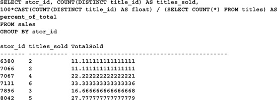
Aggregates can also appear in the HAVING clause of a query. When a query has a HAVING clause, it’s quite common for it to contain aggregates. Here’s an example:
SELECT stor_id, COUNT(DISTINCT title_id) AS titles_sold,
100*CAST(COUNT(DISTINCT title_id) AS float) / (SELECT COUNT(*) FROM titles) AS
percent_of_total
FROM sales
GROUP BY stor_id
HAVING COUNT(DISTINCT title_id) > 2

This is just a rehash of the previous query, with a HAVING clause appended to it. HAVING filters the result set in the same way that WHERE filters the SELECT itself. It’s common to reference an aggregate value in the HAVING clause since that value was not yet computed or available when WHERE was processed.
Closely related to the aggregate functions are the GROUP BY and HAVING clauses. GROUP BY divides a table into groups, and each group can have its own aggregate values. As I said earlier, HAVING limits the groups returned by GROUP BY.
With the exception of bit, text, ntext, and image columns, any column can participate in the GROUP BY clause. To create groups within groups, simply list more than one column. Here’s a simple GROUP BY example:

GROUP BY ALL generates all possible groups—even those that do not meet the query’s search criteria. Aggregate values in groups that fail the search criteria are returned as NULL. Here’s an example:
GROUP BY ALL is incompatible with the ROLLUP and CUBE operators and with remote tables. It’s also overridden by HAVING, as you might expect, in the same sense that a plain GROUP BY is overridden by it—HAVING filters what GROUP BY returns.
Notice the ORDER BY clause in the previous example. You can no longer assume that the groups returned by GROUP BY will be sorted in a particular order. This behavior differs from that of SQL Server 6.5 and earlier, so it’s something to watch out for. If you require a specific order, use ORDER BY to ensure it.
Though normally used in conjunction with aggregates, GROUP BY and HAVING don’t require them. Using GROUP BY without aggregates has the effect of removing duplicates from the data. It has the same effect as prefixing the grouping columns with DISTINCT in the SELECT list, and, in fact, SQL Server treats GROUP BY queries without aggregates and plain SELECTs with DISTINCT identically. This means that the same execution plan will be generated for these two queries:
SELECT s.title_id
FROM sales s
GROUP BY s.title_id
SELECT DISTINCT s.title_id
FROM sales s
(To view execution plans in Query Analyzer, press Ctrl-K or select Show Execution Plan from the Query menu before running your query.)
As we discovered in the earlier section on relational division, GROUP BY clauses without aggregate functions have a purpose beyond simulating SELECT DISTINCT queries. Including a GROUP BY clause, even one without aggregates, allows a result set to be filtered based on a direct reference to an aggregate. Unlike the WHERE clause, the HAVING clause can reference an aggregate without encapsulating it in a subquery. One of the relational division examples above uses this fact to qualify the rows returned by a subquery using an aggregate in its HAVING clause.
It’s pretty common to need to reshape vertically oriented data into horizontally oriented tables suitable for reports and user interfaces. These tables are known as pivot tables or cross-tabulations (cross-tabs) and are an essential feature of any OLAP (Online Analytical Processing), EIS (Executive Information System), or DSS (Decision Support System) application.
SQL Server includes a bevy of OLAP support tools that are outside the scope of this book. Install the OLAP Services from your SQL Server CD, and view the product documentation for more information.
That said, the task of reshaping vertical data is well within the scope of this book and is fairly straightforward in Transact-SQL. Let’s assume we start with this table of quarterly sales figures:
CREATE TABLE #crosstab (yr int, qtr int, sales money)
INSERT #crosstab VALUES (1999, 1, 44)
INSERT #crosstab VALUES (1999, 2, 50)
INSERT #crosstab VALUES (1999, 3, 52)
INSERT #crosstab VALUES (1999, 4, 49)
INSERT #crosstab VALUES (2000, 1, 50)
INSERT #crosstab VALUES (2000, 2, 51)
INSERT #crosstab VALUES (2000, 3, 48)
INSERT #crosstab VALUES (2000, 4, 45)
INSERT #crosstab VALUES (2001, 1, 46)
INSERT #crosstab VALUES (2001, 2, 53)
INSERT #crosstab VALUES (2001, 3, 54)
INSERT #crosstab VALUES (2001, 4, 47)
And let’s say that we want to produce a cross-tab consisting of six columns: the year, a column for each quarter, and the total sales for the year. Here’s a query to do the job:
SELECT
yr AS ’Year’,
SUM(CASE qtr WHEN 1 THEN sales ELSE NULL END) AS Q1,
SUM(CASE qtr WHEN 2 THEN sales ELSE NULL END) AS Q2,
SUM(CASE qtr WHEN 3 THEN sales ELSE NULL END) AS Q3,
SUM(CASE qtr WHEN 4 THEN sales ELSE NULL END) AS Q4,
SUM(sales) AS Total
FROM #crosstab
GROUP BY yr

Note that it isn’t necessary to total the Qn columns to produce the annual total. The query is already grouping on the yr column; all it has to do to summarize the annual sales is include a simple aggregate. There’s no need for a subquery, derived table, or any other exotic construct, unless, of course, there are sales records that fall outside quarters 1–4, which shouldn’t be possible.
The qtr column in the sample data made constructing the query fairly easy—almost too easy. In practice, it’s pretty rare for time series data to include a quarter column—it’s far more common to start with a date for each series member and compute the required temporal dimensions. Here’s an example that uses the Orders table in the Northwind database to do just that. It translates the OrderDate column for each order into the appropriate temporal boundary:

This query returns a count of the orders for each quarter as well as for each year. It uses the DATEPART() function to extract each date element as necessary. As the query iterates through the Orders table, the CASE functions evaluate each OrderDate to determine the quarter “bucket” into which it should go, then return either “1”—the order is counted against that particular quarter—or NULL—the order is ignored.
The GROUP BY clause’s CUBE and ROLLUP operators add summary rows to result sets. CUBE produces a multidimensional cube whose dimensions are defined by the columns specified in the GROUP BY clause. This cube is an explosion of the underlying table data and is presented using every possible combination of dimensions.
ROLLUP, by contrast, presents a hierarchical summation of the underlying data. Summary rows are added to the result set based on the hierarchy of grouped columns, from left to right.
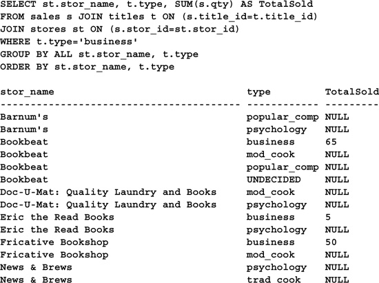
Here’s an example that uses the ROLLUP operator to generate subtotal and total rows:
SELECT CASE GROUPING(st.stor_name) WHEN 0 THEN st.stor_name ELSE ’ALL’ END AS Store,
CASE GROUPING(t.type) WHEN 0 THEN t.type ELSE ’ALL TYPES’ END AS Type,
SUM(s.qty) AS TotalSold
FROM sales s JOIN titles t ON (s.title_id=t.title_id)
JOIN stores st ON (s.stor_id=st.stor_id)
GROUP BY st.stor_name, t.type WITH ROLLUP

This query has several noteworthy features. First, note the extra rows that ROLLUP inserted into the result set. Since the query groups on the stor_name and type columns, ROLLUP produces summary rows first for each stor_name group (ALL TYPES), then for the entire result set.
The GROUPING() function is used to translate the label assigned to each grouping column. Normally, grouping columns are returned as NULLs. By making use of GROUPING(), the query is able to translate those NULLs to something more meaningful.
Here’s that same query again, this time using CUBE:
SELECT CASE GROUPING(st.stor_name) WHEN 0 THEN st.stor_name ELSE ’ALL’ END AS Store,
CASE GROUPING(t.type) WHEN 0 THEN t.type ELSE ’ALL TYPES’ END AS Type,
SUM(s.qty) AS TotalSold
FROM sales s JOIN titles t ON (s.title_id=t.title_id)
JOIN stores st ON (s.stor_id=st.stor_id)
GROUP BY st.stor_name, t.type WITH CUBE

Note the additional rows at the end of the result set. In addition to the summary rows generated by ROLLUP, CUBE creates subtotals for each type of book as well.
Without detailed knowledge of your data, it’s nearly impossible to know how many rows will be returned by CUBE. However, computing the upper limit of the number of possible rows is trivial. It’s the cross product of the number of unique values 11 for each grouping column. The “+1” is for the ALL summary record generated for each attribute. In this case, there are six distinct stores and six distinct book types in the sales table. This means that a maximum of forty-nine rows will be returned in the CUBEd result set (6+1 * 6+1). Here, there are fewer than forty-nine rows because not every store has sold every type of book.
On a related note, you’ll notice that CUBE doesn’t generate zero subtotals for book types that a particular store hasn’t sold. It might be useful to have these totals so that we can see what the store is and isn’t selling. Having the full cube creates a result set that is dimensioned more uniformly, making it easier to create reports and charts over it. Here’s a full-cube version of the last query:
SELECT
CASE GROUPING(st.stor_name) WHEN 0 THEN st.stor_name ELSE ’ALL’ END AS Store,
CASE GROUPING(s.type) WHEN 0 THEN s.type ELSE ’ALL TYPES’ END AS Type,
SUM(s.qty) AS TotalSold
FROM
(SELECT DISTINCT st.stor_id, t.type, 0 AS qty
FROM stores st CROSS JOIN titles t
UNION ALL
SELECT s.stor_id, t.type, s.qty FROM sales s JOIN titles t
ON s.title_id=t.title_id) s
JOIN stores st ON (s.stor_id=st.stor_id)
GROUP BY st.stor_name, s.type WITH CUBE


This query begins by creating a zero-value table of stores and book types by multiplying the stores in the stores table by the book types in the titles table using a CROSS JOIN. It then UNIONs this set with the sales table to produce a composite that includes the sales records for each store, as well as a zero value for each store–book type combo. This is then fed into the outer grouping query as a derived table. The outer query then groups and summarizes as necessary to produce the result set. Note that there are forty-nine rows in the final result set—exactly the number we predicted earlier.
There are a few caveats and limitations related to CUBE and ROLLUP of which you should be aware:
• Both operators are limited to ten dimensions.
• Both preclude the generation of DISTINCT aggregates.
• CUBE can produce huge result sets. These can take a long time to generate and can cause problems with application programs not designed to handle them.
As I said earlier, HAVING restricts the rows returned by GROUP BY similarly to the way that WHERE restricts those returned by SELECT. It is processed after the rows are collected from the underlying table(s) and is therefore less efficient for garden-variety row selection than WHERE. In fact, behind the scenes, SQL Server implicitly converts a HAVING that would be more efficiently stated as a WHERE automatically. This means that the execution plans generated for the following queries are identical:
SELECT title_id
FROM titles
WHERE type=’business’
GROUP BY title_id, type
SELECT title_id
FROM titles
GROUP BY title_id, type
HAVING type=’business’
In the second query, HAVING doesn’t do anything that WHERE couldn’t do, so SQL Server converts it to a WHERE during query execution so that the number of rows processed by GROUP BY is as small as possible.
The UNION operator allows you to combine the results of two queries into a single result set. We’ve used UNION throughout this chapter to combine the results of various queries. UNIONs aren’t complicated, but there are a few simple rules you should keep in mind when using them:
• Each query listed as a UNION term must have the same number of columns and must list them in the same order as the other queries.
• The columns returned by each SELECT must be assignment compatible or be explicitly converted to a data type that’s assignment compatible with their corresponding columns in the other SELECTs.
• Combining columns that are assignment compatible but of different types produces a column with the higher type precedence of the two (e.g., combining a smallint and a float results in a float result column).
• The column names returned by the UNION are derived from those of the first SELECT.
• UNION ALL is faster than UNION because it doesn’t remove duplicates before returning. Removing duplicates may force the server to sort the data, an expensive proposition, especially with large tables. If you aren’t concerned about duplicates, use UNION ALL instead of UNION.
Here’s an example of a simple UNION:
SELECT title_id, type
FROM titles
WHERE type=’business’
UNION ALL
SELECT title_id, type
FROM titles
WHERE type=’mod_cook’

This query UNIONs two separate segments of the titles table based on the type field. Since the query used UNION ALL, no sorting of the elements occurs.
As illustrated earlier in the chapter, one of the niftier features of UNION is the ability to use derived tables to create a virtual table on the fly during a query. This is handy for creating lookup tables and other types of tabular constructs that don’t merit permanent storage. Here’s an example:
SELECT title_id AS Title_ID, t.type AS Type, b.typecode AS TypeCode
FROM titles t JOIN
(SELECT ’business’ AS type, 0 AS typecode
UNION ALL
SELECT ’mod_cook’ AS type, 1 AS typecode
UNION ALL
SELECT ’popular_comp’ AS type, 2 AS typecode
UNION ALL
SELECT ’psychology’ AS type, 3 AS typecode
UNION ALL
SELECT ’trad_cook’ AS type, 4 AS typecode
UNION ALL

The query uses Transact-SQL’s ability to produce a result set without referencing a database object to construct a virtual table from a series of UNIONed SELECT statements. In this case, we use it to translate the type field in the titles table into a code. Of course, a CASE statement would be much more efficient here—we’ve taken the virtual table approach for purposes of illustration only.
The ORDER BY clause is used to sort the data in a result set. When possible, the query optimizer will use an index to service the sort request. When this is impossible or deemed suboptimal by the optimizer, a work table is constructed to perform the sort. With large tables, this can take a while and can run tempdb out of space if it’s not sized sufficiently large. This is why you shouldn’t order result sets unless you actually need a specific row order—doing so wastes server resources. On the other hand, if you need a fixed sort order, be sure to include an ORDER BY clause. You can no longer rely on clauses such as GROUP BY and UNION to produce useful row ordering. This represents a departure from previous releases of SQL Server (6.5 and earlier), so watch out for it. Queries that rely on a specific row ordering without using ORDER BY may not work as expected.
Columns can be referenced in an ORDER BY clause in one of three ways: by name, by column alias, or by result set column number. Here’s an example:

This query orders the result set using all three methods, which is probably not a good idea within a single query. As with a lot of multiflavored coding techniques, there’s nothing wrong with it syntactically, but doing something three different ways when one will do, needlessly obfuscates your code. Remember the law of parsimony (a.k.a. Ockham’s razor)—one should neither assume nor promote the existence of more elements than are logically necessary to solve a problem.
This doesn’t mean that you might not use each of these techniques at different times. The ability to reference result set columns by number is a nice shorthand way of doing so. (That said, ordering by column numbers has been deprecated in recent years, so it’s advisable to name your columns and sort using column aliases instead.) Being able to use column aliases alleviates the need to repeat complex expressions in the ORDER BY clause, and referencing table columns directly allows you to order by items not in the SELECT list.
You can also include subqueries and constants in the ORDER BY clause, though this is pretty rare. Subqueries contained in the ORDER BY clause can be correlated or stand-alone.
Each column in the ORDER BY list can be optionally followed by the DESC or ASC keyword in order to sort in descending or ascending (the default) order. Here’s an example:
SELECT st.stor_name AS Store, t.type AS Type, SUM(qty) AS Sales
FROM stores st JOIN sales s ON (st.stor_id=s.stor_id)
JOIN titles t ON (s.title_id=t.title_id)
GROUP BY st.stor_name, t.type
ORDER BY Store DESC, Type ASC

A few things to keep in mind regarding ORDER BY:
• You can’t use ORDER BY in views, derived tables, or subqueries without also using the TOP n extension (see the section on TOP n earlier in this chapter for more information). A technique for working around this is to include a TOP n clause that specifies more rows than exist in the underlying table(s).
• You can’t sort on text, ntext, or image columns.
• If your query is a SELECT DISTINCT or combines result sets via UNION, the columns listed in the ORDER BY clause must appear in the SELECT list.
• If the SELECT includes the UNION operator, the column names and aliases you can use are limited to those of the first table in the UNION.
In this chapter, you explored the ubiquitous, omnipotent Transact-SQL SELECT statement. Mastering it is essential to becoming an adroit Transact-SQL programmer. SELECT is powerful, but that power comes at a price: complexity. While SELECT statements can be very brief and concise, they are often extremely intricate in real applications.
1 Codd, E. F. 1970. “A Relational Model of Data for Large Shared Data Banks.” Communications of the ACM. New York: Association for Computing Machinery.