

At this point you should have some confidence loading binaries into IDA and letting IDA work its magic while you sip your favorite beverage. Once IDA’s initial analysis phase is complete, it is time for you to take control. One of the best ways for you to familiarize yourself with IDA’s displays is simply to browse around the various tabbed subwindows that IDA populates with data about your binary. The efficiency and effectiveness of your reverse engineering sessions will improve as your comfort level with IDA increases.
Before we dive into the major IDA subdisplays, it is useful to cover a few basic rules concerning IDA’s user interface:
- There is no undo in IDA.
If something unexpected happens to your database as a result of an inadvertent keypress, you are on your own to restore your displays to their previous states.
- Almost all actions have an associated menu item, hotkey, and toolbar button.
Remember, the IDA toolbar is highly configurable, as is the mapping of hotkeys to menu actions.
- IDA offers good, context-sensitive menu actions in response to right mouse clicks.
While these menus do not offer an exhaustive list of permissible actions at a given location, they do serve as good reminders for the most common actions you will be performing.
With these facts in mind, let’s begin our coverage of the principal IDA data displays.
In its default configuration, IDA creates seven (as of version 6.1) display windows during the initial loading-and-analysis phase for a new binary. Each of these display windows is accessible via a set of title tabs displayed immediately beneath the navigation band (shown previously in Figure 4-9). The three immediately visible windows are the IDA-View window, the Functions window, and the Output window. Whether or not they are open by default, all of the windows discussed in this chapter can be opened via the View ▸ Open Subviews menu. Keep this fact in mind, as it is fairly easy to inadvertently close the display windows.
The esc key is one of the more useful hotkeys in all of IDA. When the disassembly window is active, the esc key functions in a manner similar to a web browser’s back button and is therefore very useful in navigating the disassembly display (navigation is covered in detail in Chapter 6). Unfortunately, when any other window is active, the esc key serves to close the window. Occasionally, this is exactly what you want. At other times, you will immediately wish you had that closed window back.
Also known as the IDA-View window, the disassembly window will be your primary tool for manipulating and analyzing binaries. Accordingly, it is important that you become intimately familiar with the manner in which information is presented in the disassembly window.
Two display formats are available for the disassembly window: the default graph-based view and a text-oriented listing view. Most IDA users tend to prefer one view over the other, and the view that better suits your needs is often determined by how you prefer to visualize a program’s flow. If you prefer to use the text listing view as your default disassembly view, you can change the default by using the Options ▸ General dialog to turn off Use graph view by default on the Graph tab. Whenever the disassembly view is active, you can easily switch between graph and listing views at any time by using the spacebar.
Figure 5-1 shows a very simple function displayed in graph view. Graph views are somewhat reminiscent of program flowcharts in that a function is broken up into basic blocks[34] so you can visualize the function’s control flow from one block to another.
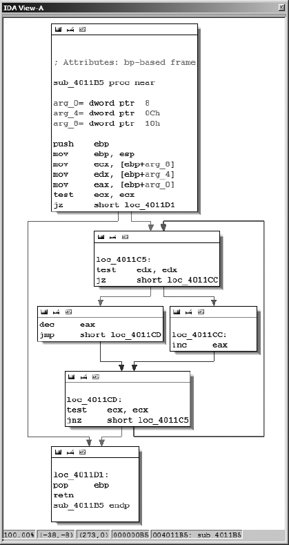
Onscreen, you’ll notice IDA uses different colored arrows to distinguish various types of flows[35] between the blocks of a function. Basic blocks that terminate with a conditional jump generate two possible flows depending on the condition being tested: the Yes edge arrow (yes, the branch is taken) is green by default, and the No edge arrow (no, the branch is not taken) is red by default. Basic blocks that terminate with only one potential successor block utilize a Normal edge (blue by default) to point to the next block to be executed.
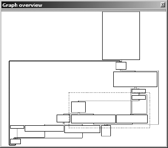
In graph mode, IDA displays one function at a time. For users with a wheel mouse, graph zooming is possible using the ctrl- wheel combination. Keyboard zoom control requires ctrl-+ to zoom in or ctrl- − to zoom out (using the + and − keys on the numeric keypad). Large or complex functions may cause the graph view to become extremely cluttered, making the graph difficult to navigate. In such cases, the Graph Overview window (see Figure 5-2) is available to provide some situational awareness. The overview window always displays the complete block structure of the graph along with a dashed frame that indicates the region of the graph currently being viewed in the disassembly window. The dashed frame can be dragged across the overview window to rapidly reposition the graph view to any desired location on the graph.
With the graph display, there are several ways that you can manipulate the view to suit your needs:
- Panning
First, in addition the using the Graph Overview window to rapidly reposition the graph, you can also reposition the graph by clicking and dragging the background of the graph view.
HEY, ISN’T SOMETHING MISSING HERE?
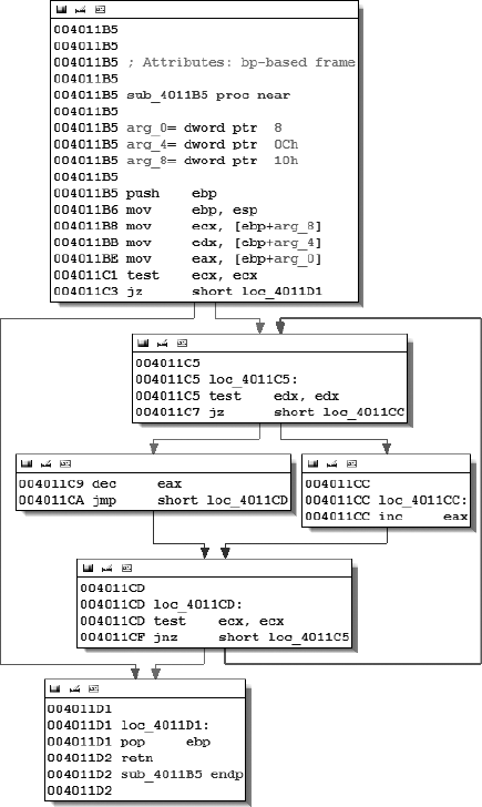
When using graph view, it may seem as if less information is available to you about each line of the disassembly. The reason for this is that IDA chooses to hide many of the more traditional pieces of information about each disassembled line (such as virtual address information) in order to minimize the amount of space required to display each basic block. You can choose to display additional information with each disassembly line by choosing among the available disassembly line parts accessible via the Disassembly tab from Options ▸ General. For example, to add virtual addresses to each disassembly line, we enable line prefixes, transforming the graph from Figure 5-1 into the graph shown in Figure 5-3.
- Rearranging blocks
Individual blocks within the graph can be dragged to new positions by clicking the title bar for the desired block and dragging it to a new position. Beware that IDA performs only minimal rerouting of any edges associated with a moved block. You can manually reroute edges by dragging vertices to new locations. New vertices can be introduced into an edge by double-clicking the desired location within an edge while holding the shift key. If at any point you find yourself wishing to revert to the default layout for your graph, you can do so by right-clicking the graph and choosing Layout Graph.
- Grouping and collapsing blocks
Blocks can be grouped, either individually or together with other blocks, and collapsed to reduce the clutter in the display. Collapsing blocks is a particularly useful technique for keeping track of blocks that you have already analyzed. You can collapse any block by right-clicking the block’s title bar and selecting Group Nodes.
- Creating additional disassembly windows
If you ever find yourself wanting to view graphs of two functions simultaneously, all you need to do is open another disassembly window using Views ▸ Open Subviews ▸ Disassembly. The first disassembly window opened is titled IDA View-A. Subsequent disassembly windows are titled IDA View-B, IDA View-C, and so on. Each disassembly is independent of the other, and it is perfectly acceptable to view a graph in one window while viewing a text listing in another or to view three different graphs in three different windows.
Keep in mind that your control over the view extends beyond just these examples. Additional IDA graphing capabilities are covered in Chapter 9, while more information on the manipulation of IDA’s graph view is available in the IDA help file.
The text-oriented disassembly window is the traditional display used for viewing and manipulating IDA-generated disassemblies. The text display presents the entire disassembly listing of a program (as opposed to a single function at a time in graph mode) and provides the only means for viewing the data regions of a binary. All of the information available in the graph display is available in the text display in one form or another.
Figure 5-4 shows the text view listing of the same function shown in Figure 5-1 and Figure 5-3. The disassembly is presented in linear fashion, with virtual addresses displayed by default. Virtual addresses are typically displayed in a [SECTION NAME]:[VIRTUAL ADDRESS] format such as .text:004011C1.
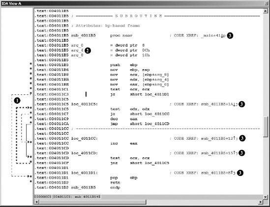
The left portion of the display, seen at ![]() , is called the arrows window and is used to depict nonlinear flow within a function. Solid arrows represent unconditional jumps, while dashed arrows represent conditional jumps. When a jump (conditional or unconditional) transfers control to an earlier address in the program, a heavy weighted line (solid or dashed) is used. Such reverse flow in a program often indicates the presence of a loop. In Figure 5-4, a loop arrow flows from address
, is called the arrows window and is used to depict nonlinear flow within a function. Solid arrows represent unconditional jumps, while dashed arrows represent conditional jumps. When a jump (conditional or unconditional) transfers control to an earlier address in the program, a heavy weighted line (solid or dashed) is used. Such reverse flow in a program often indicates the presence of a loop. In Figure 5-4, a loop arrow flows from address 004011CF to 004011C5.
The declarations at ![]() (also present in graph view) represent IDA’s best estimate concerning the layout of the function’s stack frame.[36] IDA computes the structure of a function’s stack frame by performing detailed analysis of the behavior of the stack pointer and any stack frame pointer used within a function. Stack displays are discussed further in Chapter 6.
(also present in graph view) represent IDA’s best estimate concerning the layout of the function’s stack frame.[36] IDA computes the structure of a function’s stack frame by performing detailed analysis of the behavior of the stack pointer and any stack frame pointer used within a function. Stack displays are discussed further in Chapter 6.
The comments (a semicolon introduces a comment) at ![]() are cross-references. In this case we see code cross-references (as opposed to data cross-references), which indicate that another program instruction transfers control to the location containing the cross-reference comment. Cross-references are the subject of Chapter 9.
are cross-references. In this case we see code cross-references (as opposed to data cross-references), which indicate that another program instruction transfers control to the location containing the cross-reference comment. Cross-references are the subject of Chapter 9.
For the remainder of the book we will primarily utilize the text display for examples. We’ll use the graph display only in cases where it may provide significantly more clarity. In Chapter 7 we will cover the specifics of manipulating the text display in order to clean up and annotate a disassembly.
The Functions window is used to list every function that IDA has recognized in the database. A Functions window entry might look like the following:
malloc .text 00BDC260 00000180 R . . . B . .
This particular line indicates that the malloc function can be found in the .text section of the binary at virtual address 00BDC260, is 384 bytes (hex 180) long, returns to the caller (R), and uses the EBP register (B) to reference its local variables. Flags used to describe a function (such as R and B above) are described in IDA’s built-in help file (or by right-clicking a function and choosing Properties. The flags are shown as editable checkboxes in the resulting Properties dialog).
As with other display windows, double-clicking an entry in the Functions window causes the disassembly window to jump to the location of the selected function.
The Output window at the bottom of the IDA workspace rounds out the default set of windows that are visible when a new file is opened. The Ouput window serves as IDA’s output console and is the place to look for information on tasks IDA is performing. When a binary is first opened, for example, messages are generated to indicate both what phase of analysis IDA is in at any given time and what actions IDA is carrying out to create the new database. As you work with a database, the Output window is used to output the status of various operations that you perform. The contents of the Output window can be copied to the system clipboard or cleared entirely by right-clicking anywhere in the window and selecting the appropriate operation. The Output window will often be the primary means by which you display output from any scripts and plug-ins that you develop for IDA.
[34] A basic block is a maximal sequence of instructions that executes, without branching, from beginning to end. Each basic block therefore has a single entry point (the first instruction in the block) and a single exit point (the last instruction in the block). The first instruction in a basic block is often the target of a branching instruction, while the last instruction in a basic block is often a branch instruction.
[35] IDA uses the term flow to indicate how execution can continue from a given instruction. A normal (also called ordinary) flow indicates default sequential execution of instructions. A jump flow indicates that the current instruction jumps (or may jump) to a nonsequential location. A call flow indicates that the current instruction calls a subroutine.
[36] A stack frame (or activation record) is a block of memory, allocated in a program’s runtime stack, that contains both the parameters passed into a function and the local variables declared within the function. Stack frames are allocated upon entry into a function and released as the function exits. Stack frames are discussed in more detail in Chapter 6.