In this chapter, a guide is presented on a quick start to programming the Arduino, including how to install the Arduino programming environment, connect the Arduino Uno board to a host computer, and understand the basic structure of an Arduino program. The Arduino has a vast capability, and programming can get rather sophisticated. Many books have been written on programming the Arduino, ranging in skill level from beginner’s guides for students to advanced applications for professional engineers. However, the description in this chapter is rather simple, with the intent to understand just enough about programming to get the Arduino working in LEGO-based designs. The Arduino programs, called sketches, used throughout this book are adapted from various manufacturers of sensors and devices, who provide sketches specifically for their products. It’s sufficient to simply learn the rudiments of Arduino programming so that these premade sketches can be put to use.
Installing the Arduino Integrated Development Environment (IDE)
The Arduino programming utility is called Integrated Development Environment (IDE), with options available for Windows, Mac OS, and Linux operating systems. Download of the IDE can be found at www.Arduino.cc/en/Main/Software, such as in the screenshot of Figure 3-1. Upgrades are released every few months to the IDE, as identified by the version number, such as version 1.8.12 seen in Figure 3-1. Most of these upgrade changes are rather minor, with no effect on high-level programming used throughout this book.
Figure 3-1
The download page for the Arduino IDE shows options for several host computer operating systems
Navigating the Arduino IDE
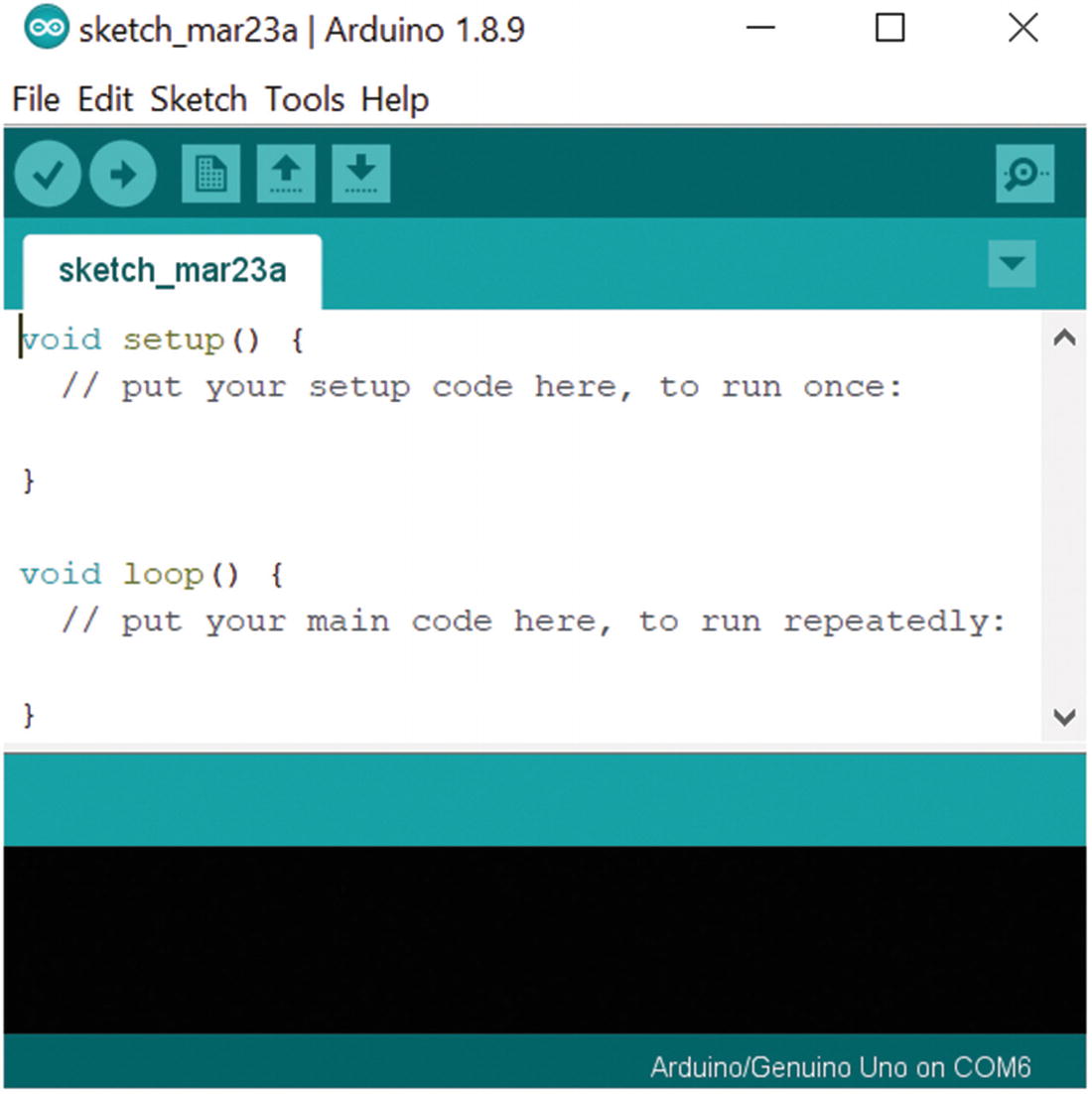
Opening the IDE will bring up a work area, as pictured in the screenshot of Figure 3-2. The large area in the center of the IDE is for the development of sketches with two sets of commands, as noted in the comments on the IDE screen: the setup for programming commands that run once and loop for commands that run in a continuous repetition. The IDE also includes utilities for saving and downloading sketches onto the Arduino board, as described in the following sections.
Figure 3-2
The IDE provides for the development of sketches and their download to the Arduino
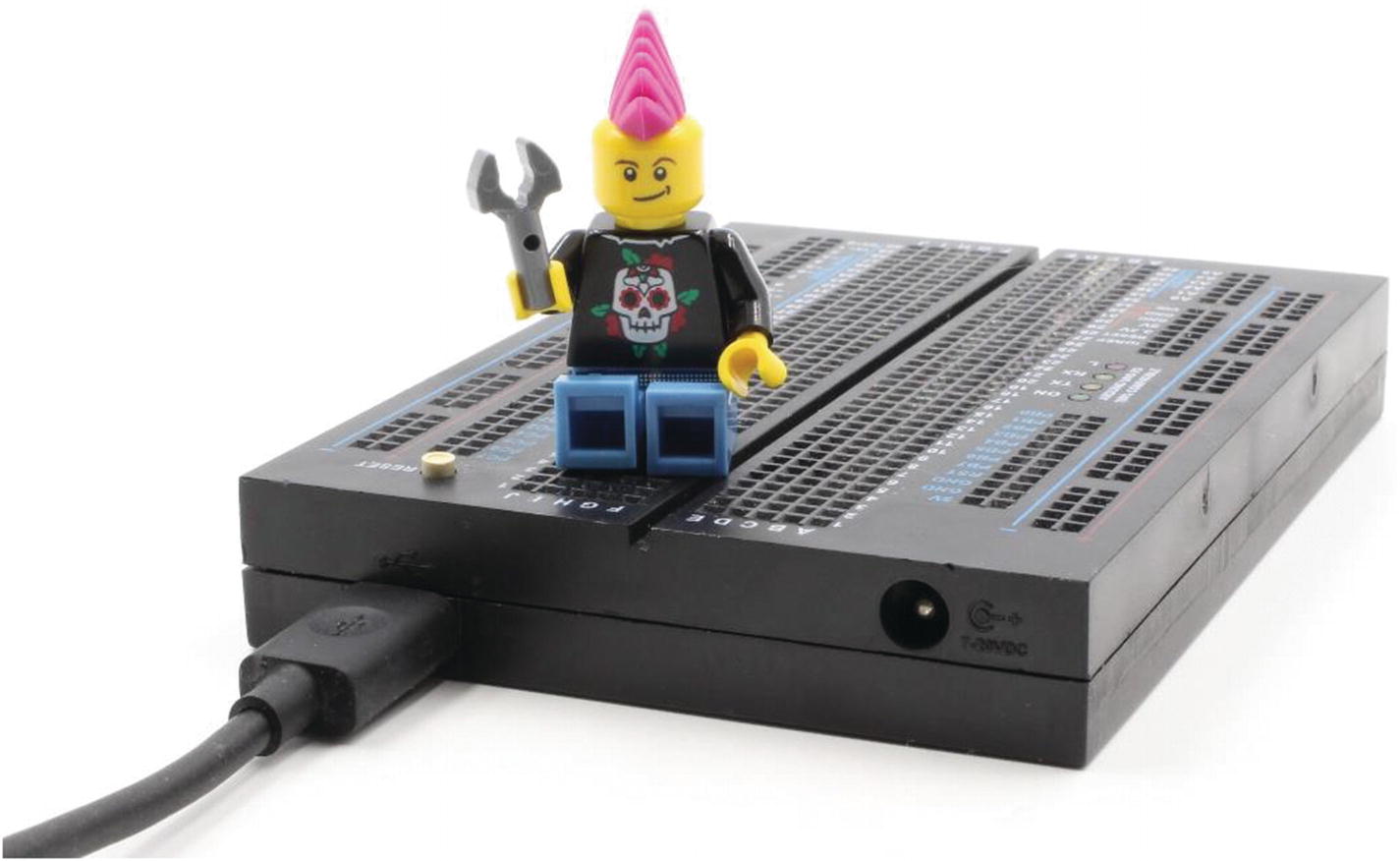
The first tab to consider from the toolbar is Tools, after connecting the Arduino board to the host computer by a USB cable. Figure 3-3 shows the micro-USB connection on the Arduino board, using a STEMTera board as an example.
Figure 3-3
Connection of the Arduino to a host computer is by a USB connection
Once the Arduino is physically connected, it should show up in the IDE under Tools ➤ Port, as pictured in Figure 3-4. The Arduino is recognized by the Arduino/Genuino Uno name following the assigned Port. A further diagnostic on a correct connection can be found under Tools ➤ Get Board Info, with a positive result being a pop-up screen showing addresses and serial number associated with the Arduino.
Figure 3-4
Connection to the Arduino can be confirmed by checking the Port connection
Running a First Sketch
Figure 3-5 shows a short program to introduce ideas in programming the Arduino with IDE. A line of code has been put into the setup section with the command:
Serial.begin(9600); //Start serial communication
Figure 3-5
A sketch for printing over a serial connection
Since this command is the setup section, it runs only once, serving here to initialize communication between the Arduino and the host computer. The 9600 indicates a baud rate, a speed at which communication takes place. The end of a command is indicated with a semicolon. The // indicates the start of a comment, which continues to the end of the current line.
The loop section runs over and over again, in this case printing “Hello!” every second over a serial communication link. Two commands accomplish this:
Serial.println("Hello!"); //Print to serial
delay(1000); //Pause for 1 second
Just as in the setup section, commands in the loop section end with a semicolon. The numeral in the delay command is in milliseconds, creating a pause in this example of 1 second.
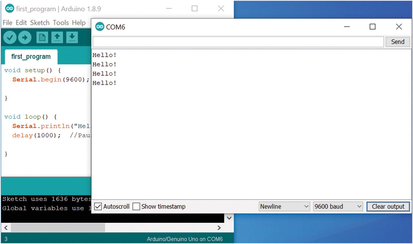
Once the program commands have been written, the sketch can be uploaded and executed by clicking the Upload icon (an arrow pointing right) on the toolbar. The results of this program can be viewed by going to the toolbar in the IDE to select Tools ➤ Serial Monitor, as shown in Figure 3-6. The word “Hello!” is printed every 1 second. An important feature in the Serial Monitor is the baud setting, which has to match the baud rate set in the sketch, 9600 in this case.
Figure 3-6
Opening the Serial Monitor should show “Hello!” printed every 1 second
More sophisticated programs will be used in the upcoming chapters of this book, adapted from various websites to be run in the IDE. A sketch can be copied from a website and then pasted inside the IDE. The Serial Monitor will be used in several of the projects of this book as a diagnostic, showing sensor readings as a check for proper operation.
Working with Libraries
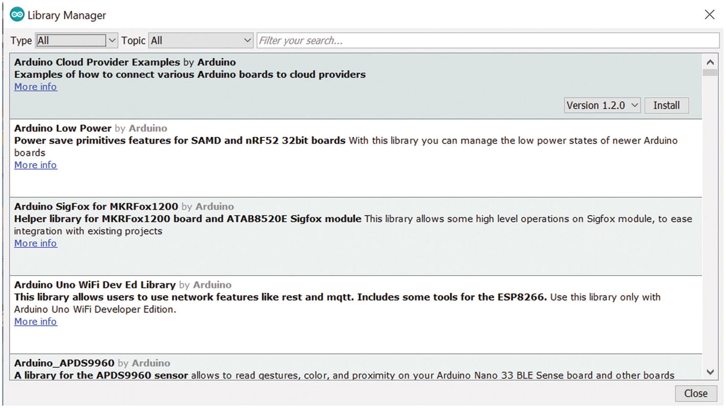
Many sensors and devices that connect to the Arduino have sets of commands written for them in the form of a Library. Arduino sketches often make use of these Libraries to work with external devices, calling up advanced functions with simple commands. Libraries can be found in the IDE by going to the toolbar to select Tools ➤ Manage Libraries, which brings up the screen shown in Figure 3-7. A particular Library of interest has to be installed into the IDE by clicking the Install link that appears in the Library listing. The Library for a particular sensor or device can be found by typing the device’s name into the search window near the top of the Library Manager.
Figure 3-7
Libraries are installed from the Library Manager
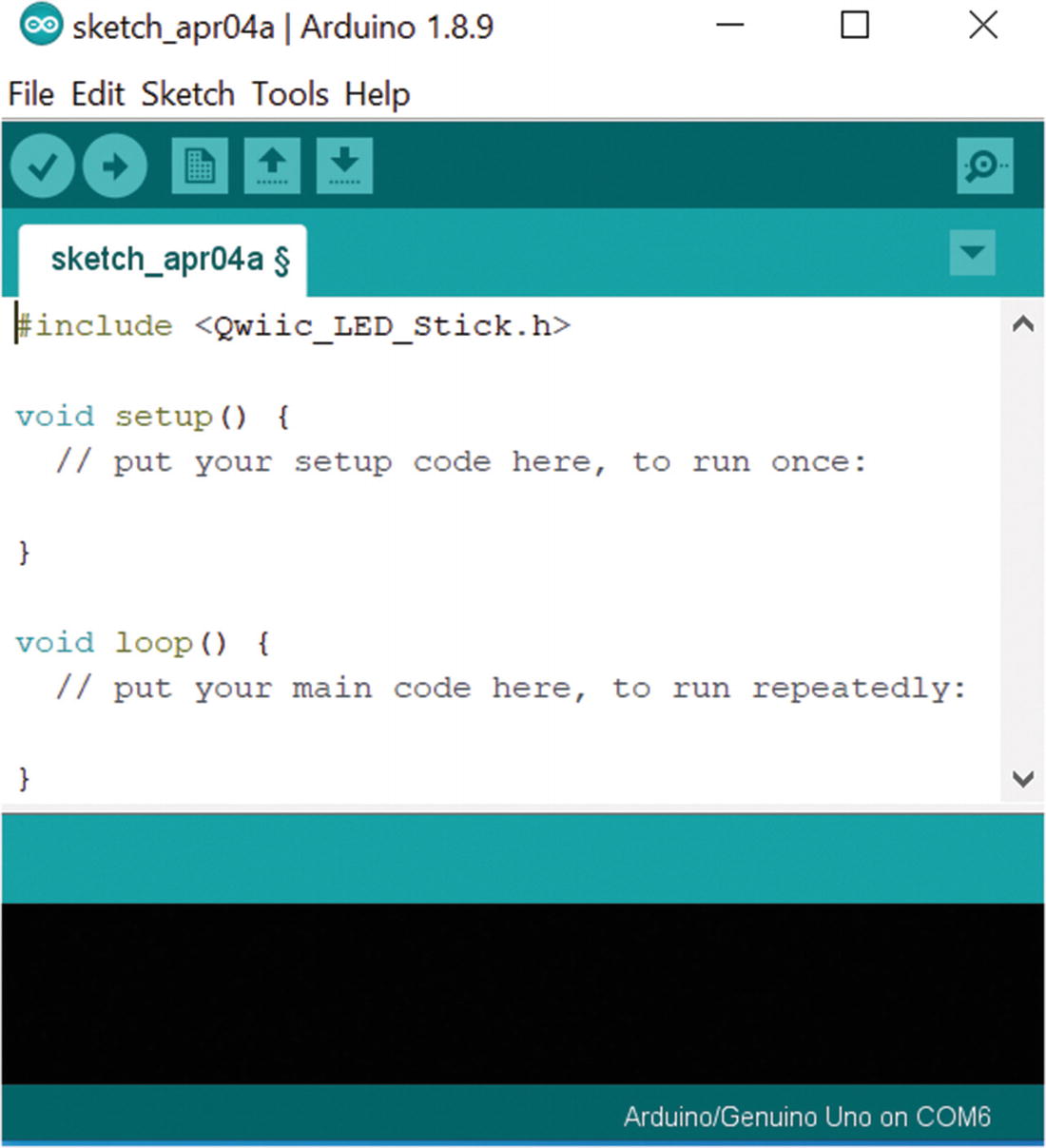
Once the Library is installed in the IDE, the Library gets called into the sketch by the command # include, such as in Figure 3-8, where the Library is being called that controls the Qwiic LED Stick used in Chapter 6. The # include command goes before the setup section of a sketch. A Library can be accessed in various places in a sketch to program sensor or device functions with a single line of code. Example commands, taking the Qwiic LED Stick of Chapter 6 as an example, are LEDStick.begin() or LEDStick.LEDoff().
Figure 3-8
A Library gets called into a sketch by the # include command
The details on how Libraries work or how to call subroutines aren’t critical to understand for the projects in this book. These details are handled within the sketches available for use from sensor manufacturers and experienced users. However, as described in this section, the Libraries need to be installed into the Arduino IDE for these copy-pasted sketches to function.
Working with Functions
A function in an Arduino sketch is a subroutine often used when a section of code is needed several times. It is analogous to a My Block in EV3 code. Using a function can cut down on program complexity if the same code is used repeatedly in a sketch. Figure 3-9 shows a sketch that adds two numbers. The two numbers to add are first defined at the beginning of the sketch, using int to declare these numbers as variables. The function, called simpleAddFunction in this example, is written at the bottom of the sketch, after the loop section of code. And in the loop itself, the function is called, with the values x and y passed to the function to return the sum. The variables defined in the function are called a and b as a placeholder for values that will be passed by the main section of the sketch—x and y are the values passed to the function in this example. This simple example, meant to show the structure and use of a function, isn’t really necessary for such a simple operation. However, as will be seen in the examples of this book, a function may be called multiple times, simplifying the sketch. Some projects make use of multiple functions, with each of the functions appearing after the sketch’s loop.
Figure 3-9
The function, named simpleAddFunction in this example, appears at the bottom of the sketch
Summary
This chapter gave a quick-start guide to programming the Arduino via the Integrated Development Environment (IDE). The IDE is installed on a host computer for connection to the Arduino Uno by a USB cable. Arduino programs are called sketches, featuring two main parts: a setup for executing commands once and a loop for infinite repetition of commands. If the program uses variables, they are declared before the setup section. A simple program was presented to demonstrate a connection to an Arduino. Building sophisticated programs is not described in this book, using instead sketches developed by sensor and device manufacturers that can be copied and pasted into the IDE. These premade sketches often involve the use of Libraries, so a primer was given on how to find and install a Library for a particular device. Sketches also often make use of functions for efficient programs, so an introduction was also given on functions.