Chapter 4. Block Diagram

The LabVIEW block diagram excels at conveying source code. A really good diagram is enlightening, even awe-inspiring, like a work of art. A careless diagram, however, can appear as jumbled as a bowl of spaghetti. Indeed, these two extremes are depicted by Meticulous VI and Spaghetti VI in Chapter 1, “The Significance of Style.” Somewhere in the middle between artwork and spaghetti is where most applications reside. Some developers have neat wiring practices but large, flat diagrams. Others have overly modular diagrams that disguise the architecture. Still others prefer variables over data flow. Many, many developers skimp on documentation to save time. Moreover, most diagrams are characterized by tradeoffs between good style and shortcuts deemed necessary to get the job done. The overall outcome is a compromise among attractive appearance, personal preferences, and functional performance.

Many developers wrongfully assume that attractive diagrams require a level of toil that is impractical for real-world applications that have tight deadlines. It seems faster and more productive to avoid getting caught up in diagram aesthetics. Indeed, it is possible to expend excessive time optimizing the appearance of a complex diagram, and most of us must plead guilty for doing this on occasion. However, it is always much more time consuming, in the long run, to debug and modify sloppy code. Per Theorem 1.1, applying good style significantly reduces time and effort throughout an application’s life cycle. Additionally, neat development practices need not be overly time consuming. If you know the style rules and how to implement them, you eliminate the toil.

This chapter presents style rules that ensure neat and organized diagrams that are practical to implement in real applications with tight deadlines. Combined with the rules in other chapters, they ensure readable and maintainable LabVIEW source code. Moreover, mastery of these style rules may lead to awe-inspiring LabVIEW diagrams.

4.1 Layout

This section covers rules for block diagram layout, including layout basics, and subVI modularization.

4.1.1 Layout Basics

The following rules pertain to the general layout of the block diagram.

The display resolution affects the visible area the developer has to work with and how the diagram appears when opened on a given target computer. It is beneficial to standardize on one display resolution so that the diagram window maintains a consistent appearance when opened on PCs with similar display capabilities. The higher the resolution setting, the smaller the diagram objects shrink relative to the screen size, and the more code fits on one screen. A fairly high resolution is recommended to maximize the viewable diagram area without straining your eyes. The LabVIEW development environment is designed for a minimum 1024×768 resolution. A resolution of 1280×1024 provides additional real estate while maintaining compatibility with mainstream PC display technology. Avoid resolutions much higher than 1280×1024 because higher resolutions are less universally supported, and the larger work area promotes larger diagrams and potentially less modularity. Also, depending on the monitor size, very high resolutions may strain your eyes. Although I have 20/20 vision, several years ago, I went through a phase where I wore tinted prescription glasses during LabVIEW development. An adjustment to the resolution setting, along with general improvements in display technology, eliminated this problem for me.

Today many computers support multiple monitors. It is particularly useful to utilize two monitors for LabVIEW development. This allows you to dedicate one monitor to the front panel and the other monitor to the block diagram, and have both windows simultaneously visible without having to navigate between them.

Do not color the diagrams. Leave the background of the diagram, and every subdiagram of every structure, default white. Data flow must be easy to visualize. A high density of objects is desired, without crowding objects too close and causing wires and objects to overlap. In general, try to limit the diagram size to one display screen. In some situations, it is difficult to work within this constraint, such as a complex diagram containing multiple parallel loops. In this case, organize the large diagram so that it may be viewed by scrolling in only one direction, or modularize the loops into subVIs to reduce space. Loop-subVIs are discussed in Chapter 8, “Design Patterns.” Avoid large diagrams that require both horizontal and vertical scrolling because this is cumbersome to navigate.

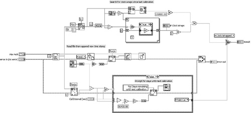
Figure 4-1 contains two functionally equivalent implementations of a VI that evaluates a calibration interval. The diagram of Figure 4-1A is overly dense and sloppy. As you can see, several of the functions and wires overlap, and the diagram appears confusing. In Figure 4-1B, the same VI is revised for improved readability. The functions are neatly spaced, the wiring is clear, a few comments and enumerations are included, and the error cluster propagates throughout the diagram. The implementation of Figure 4-1B is much more readable than Figure 4-1A. We revisit this example very shortly.

Figure 4-1A. The diagram for a VI that evaluates a calibration interval is overly dense and confusing.

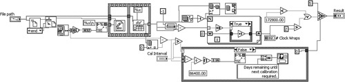
Figure 4-1B. A different implementation of the Calibration Interval VI contains appropriate spacing, clear wiring, and documentation.

4.1.2 SubVI Modularization

If your diagrams commonly extend beyond one window, maximized on a monitor with 1280×1024 resolution, your source code is not sufficiently modular. If the Navigation Window is integral to your development, you definitely need more subVIs!

• Strive for a modularity index greater than 3.0

Develop your applications as a multilayer hierarchy of subVIs using a combination of top-down and bottom-up design and development techniques. The VI Hierarchy is viewed by selecting View»VI Hierarchy. Deselect Include VI Lib, Include Globals, and Include typedef from the toolbar to remove these items from the window, and view only the hierarchy of user VIs that you provided. Common geometries include pyramid, diamond, and oval. Except for very simple applications, the VI Hierarchy should contain multiple rows of subVIs below the top-level VI. In Chapter 1, the modularity index was defined as the ratio of the number of user VIs to total nodes, multiplied by 100. These quantities are quickly referenced using the VI Metrics window, selected from Tools»Profile»VI Metrics. A modularity index of 3.0 or greater is recommended for a typical application.

• Develop high-level component VIs

• Replace collections of Property Nodes with Control References and subVIs

Depending on the design pattern, most top-level diagrams should consist of structures, wires, component VIs, and subVIs. Component VIs are very high-level subVIs, or dynamically loaded plug-in VIs, that encapsulate a major portion or subsystem of the application. An application’s graphical user interface and data acquisition engine, implemented as separate VIs, are examples of component VIs. The top-level and high-level diagrams should contain very few low-level data-manipulation functions, such as math, array manipulations, string formatting, and similar functions.

Some applications require large numbers of Property Nodes for controlling GUI behavior. Most Property Node read and write operations are triggered by GUI events. Consequently, the Event structure is an ideal construct for handling Property Nodes. Because the Event structure contains separate subdiagrams for each event case, it is uncommon to run out of space. However, it is common to have multiple event cases that require many of the same Property Nodes, with different values read or written to them in each. Modularize these common Property Nodes into subVIs, and pass the Control References and property values to the subVI in each location. Each instance of the subVI refers to the same collection of Property Nodes in memory. This substantially reduces memory use and diagram complexity.

• Modularize low-level routines into cohesive subVIs

• Use or develop instrument drivers and utility VIs

Likewise, modularize the diagrams of your high-level component VIs into lower-level subVIs. Using the top-down design and development approach, modularize any low-level routines into cohesive subVIs. Anywhere you have a collection of related functions that work together to perform a specific routine, replace them with a subVI. A subVI is cohesive if you can clearly describe its purpose in two or three sentences, such as when entering the subVI’s description.

Also, using the bottom-up approach, develop or reuse instrument drivers and utility VIs. Instrument drivers encapsulate the low-level device communications, including command string assembly, VISA functions, and response string parsing. Utility VIs complement or extend the capabilities of the built-in LabVIEW functions and VIs available on the Functions palette. Thousands of reusable instrument drivers and utility VIs are available for free download on the Web¹. Code reuse is discussed in Chapter 2, “Prepare for Good Style.”

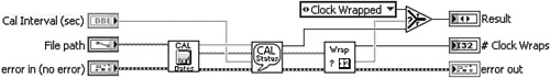
In Figure 4-2, we revisit the calibration interval diagram from Figure 4-1. This is an example of a high-level subVI. Inspecting Figure 4-2A, we observe three low-level routines: reading and appending the time stamps to file, searching and counting clock wraps, and prompting the number of days until the next calibration. In Figure 4-2B, each routine is modularized into a cohesive subVI. The subVIs remain in the same respective locations as the code they encapsulate. In Figure 4-2C, the three subVIs are placed in series, the error cluster propagates between each subVI, and the Merge Errors VI is eliminated. The resulting diagram is now a simple set of three subVI calls. We can see that the diagram is much neater, simpler, and organized with subVIs.

Figure 4-2A. The calibration interval VI contains three routines.

Figure 4-2B. Each routine is modularized into cohesive subVIs.

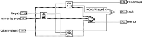
Figure 4-2C. The subVIs are rearranged into a dataflow sequence that propagates the error cluster and reduces wire clutter.

SubVIs are advantageous because it is easier to develop, test, debug, maintain, and reuse software modules as subVIs versus sections of a large diagram. As shown in Figure 4-2C, they also provide a considerable space-saving benefit. In general, if the collection of functions or Property Nodes or other routine is used in more than one place, it is an easy decision: Replace the repeated code with a subVI. Likewise, if several nonrepetitive nodes are related to one another and work together to perform a specific task, modularize them into cohesive subVIs, whether they are needed in multiple places or not. However, do not randomly select areas of the diagram and create subVIs just to save space. SubVIs created in this manner are not cohesive, intuitive, or reusable. Also, do not create trivial subVIs that contain few nodes. In this case, the subVI icon unnecessarily masks the underlying code on the diagram. For example, the subVI in Figure 4-3 contains only a single Index Array function. However, the subVI’s icon, name, and description disguise the function. The LabVIEW functions and shipping subVIs within vi.lib are universally recognizable, so avoid masking them within trivial subVIs.

Figure 4-3. This subVI contains too few nodes. Its icon, name, and description disguise the Index Array function on the diagram of the calling VI.

Always create a meaningful icon and cohesive description for every subVI. I cannot emphasize this enough. At Bloomy Controls, this is one of our most sacred precepts. The icon and description identify the subVI from the diagram of the calling VI through the Context Help window. The description enforces the cohesion test. If you cannot summarize its purpose in two or three sentences, it probably contains too much code for one subVI. Icons and descriptions are discussed in more detail in Chapter 5, “Icon and Connector,” and Chapter 9, “Documentation,” respectively.

4.2 Wiring

This section covers rules for wiring, including clear wiring techniques, and cluster modularization.

4.2.1 Clear Wiring Techniques

The fewer bends, kinks, and loops your wires have, the more fluid your diagrams appear. There are manual and automatic methods of wire routing and cleaning. I prefer manual wire routing because the automatic methods prioritize horizontal terminal entries and avoiding overlaps, at the expense of creating extra bends. To minimize the bends, it is necessary to route wires manually. Auto wire routing can be disabled temporarily or for all new wires. To disable and enable auto wire routing on-the-fly, toggle the <A> key at any time after you initiate a new wire. To disable auto wire routing for all new wires, navigate to Tools»Options, select Block Diagram from the Category list, and deselect the Enable auto wiring check box. My preference is to first connect the wires manually and then consider repositioning nodes and individual wire segments to minimize overlaps. The result is fewer bends and overlaps. Additionally, right-click on an existing wire and select Clean Up Wire to automatically reduce kinks, loops, and bends.

When propagating parallel wires, maintain consistent, even spacing between each node or bend. There are two useful techniques for ensuring even spacing. First, use similar connector pattern and terminal assignments for all subVIs that are intended to be used together. Connector pattern conventions are covered in Chapter 5. Second, align the nodes horizontally before wiring. Simply select the nodes and choose any of the horizontal alignment tools from the Align Objects menu on the toolbar. In Figure 4-4, a data logging routine is developed using several File I/O functions that comprise a dataflow sequence. The file refnum and error cluster are propagated using parallel wires. The File I/O functions have similar connector patterns, which helps facilitate even spacing. However, even slight offsets in the horizontal alignment cause wire kinks. In Figure 4-4A, the diagram is initiated by dropping the functions from the palettes onto the diagram. In Figure 4-4B, the Bottom Edges alignment tool snaps the nodes into perfect horizontal alignment. You can also distribute the nodes with even horizontal gap using the horizontal distribution tool. In this example, an asymmetric horizontal gap is desired to provide extra spacing within the While Loop. In Figure 4-4C, clear wiring proceeds with even vertical spacing, without kinks or bends. In Figure 4-4D, the wiring is completed and the horizontal gaps between nodes are manually adjusted.

Figure 4-4A. A data logging routine consists of several functions containing similar connector patterns and terminal assignments.

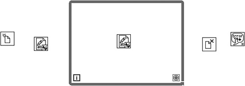
Figure 4-4B. The functions are aligned horizontally using the Bottom Edges alignment tool.

Figure 4-4C. Wires for file refnum and error cluster proceed with even spacing and without kinks or bends.

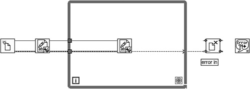
Figure 4-4D. The wiring is completed and the horizontal gaps between nodes are manually adjusted.

Tunnel wires into structures through their left border, and out of structures through their right border. Avoid tunneling wires through the top and bottom borders. Also avoid passing wires through structures if they are not utilized within the structure, unless their purpose is clearly labeled. It is particularly annoying to flip through many frames of a multiframe structure, such as a Case or an Event structure, searching for places where the data in the wire is modified. However, sometimes it is useful to pass a few spare wires through a Case structure, such as the state machine design patterns that are discussed in Chapter 8. This practice reduces maintenance when additional wires are needed. Be sure to clearly label unused wires as Unused, or Spare.

• Avoid overlapping diagram objects

Avoid obstructing the view of wires and nodes by overlapping them on the diagram. An occasional crossover of a wire routed horizontally with a wire routed vertically is unavoidable. For example, sometimes it is necessary to wire the iteration terminal of a looping structure, normally located at the bottom left of the structure, to a location above and to the right. Many of these same loops have wires routed horizontally across the entire structure, via either tunnels or shift registers. The error cluster is a prime example. If the iteration terminal is to remain on the bottom left, there may be no choice but to cross over the horizontal wires. The obstruction is minimized if the vertical wire is routed through a location of minimum wire density, overlapping as few wires as possible. Additionally, never overlap a wire with an object or a node. A wire running underneath a function or subVI resembles an input and output to the node.

Ideally, the source and destination of every wire should be readily visible without scrolling the diagram window. However, this is not always possible, even if the diagram is limited to one screen. For example, the terminals may be hidden within the frames of a multiframe structure. In this situation, be sure to label the wire in the frames or areas where the source terminal is not visible. While limiting wire lengths is desirable, long wires are preferred over no wires. Never use local or global variables as a method of reducing wire clutter. Variables increase processing overhead, memory use, and complexity. Moreover, variables undermine LabVIEW’s dataflow principles by obscuring the actual source of the data. When variables are written and read from more than one location on the diagram, it becomes difficult to determine what is actually affecting the data. When wires are used, it is easy to trace the data to its unique source terminal. If the wires are long or the data source terminal is hidden, label them. Indicate the name of the wire’s data source so that it is readily apparent when you view the diagram. Use the greater than sign (>) to reinforce the direction of data flow. Considerations with respect to local and global variables are discussed in Section 4.3, “Data Flow.”

Place any unwired terminals of front panel objects in a consistent location on the diagram so that developers can find them easily. Note that any terminals not contained by a repeating structure are read only once. This is a problem for Boolean controls configured with latching action. In this case, the control is not able to reset itself. If the terminal’s control is associated with an event that is registered by an Event structure, place the terminal within the corresponding event case. This ensures that the terminal’s value will be read each time the event fires. For unwired terminals not associated with any events, simply place them to the left of the diagram’s primary structure.

4.2.2 Cluster Modularization

It is much easier to implement clear wiring techniques and maintain organized diagrams if you reduce the overall number of wires you have to work with. Use clusters to group related data and reduce the quantity of wires. Wherever you have several wires of related data that are needed in the same areas of your diagrams, replace the individual wires with a cluster. This is analogous to modularizing low-level routines into cohesive subVIs. The data elements in the cluster should be related and serve a common purpose.

For example, consider the measurement routine from an optical filter test application, shown in Figure 4-5. The application prompts the user to define the laser scan parameters, configures a wavelength tunable laser source, measures the filter’s transmission characteristics, graphs the data, and saves the data to file. Figure 4-5A contains the panel, nonvisible indicators, and Context Help window for Define Scan VI, the dialog used for selecting the laser scan parameters. This is the first subVI called in the measurement sequence shown in Figure 4-5B. Define Scan VI provides multiple parameters used by the subsequent VIs. As shown in the Context Help window, the connector pane is densely populated with individual terminal assignments for each parameter. In Figure 4-5B, there are many individual wires flowing through a relatively simple routine. The subVI connector terminal for Save Scan VI, the last subVI in the dataflow sequence, is also very densely populated. The wiring is kept reasonably neat because of even spacing and judicious terminal assignments. However, much toil is required to achieve this result, and even more toil is required to modify the VI. Specifically, any change to the required measurement parameters entails changes to the wires, subVIs, and connectors throughout the diagram.

Figure 4-5A. Define Scan VI is a dialog that prompts the user to specify laser scan parameters. It returns 15 parameters through separate connector terminals for each.

Figure 4-5B. An optical filter measurement routine calls Define Scan VI and propagates the laser scan parameters using individual wires. The subVI connector panes are densely populated, wiring is cluttered, and maintenance is tedious.

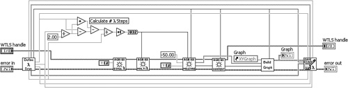
Figure 4-5C contains an alternative implementation of Define Scan VI, with the laser scan parameters returned as a cluster. In Figure 4-5D, the measurement routine is revised using the cluster instead of individual wires. Wire clutter and development toil are substantially reduced. Additionally, parameters can be added and removed from the cluster without requiring any changes to the wires and subVI connector terminal assignments. Hence, clusters improve the diagram’s appearance while reducing overall development and maintenance effort.

Figure 4-5C. Define Scan VI modularizes the laser scan parameters into a cluster. Terminal assignments are simplified.

Figure 4-5D. The cluster of laser scan parameters propagates throughout the diagram. Wire clutter is reduced. Parameters can be added and removed from the cluster without affecting wiring and subVI terminals assignments.

In some situations, it makes sense to define a cluster for just two data elements. A small cluster is useful to associate data that is very closely related and is frequently used together. As an example, the high and low limits of a measured parameter may be read from a database, edited by the user in a dialog VI, passed to another routine that compares the measured data to the limits, and passed to additional routines where a report is generated and the data and limits are logged to file. A two-element cluster containing the high and low limits eliminates one wire and logically binds the data together. In this case, the cluster is more beneficial for associating related data than for eliminating wire clutter.

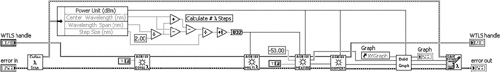
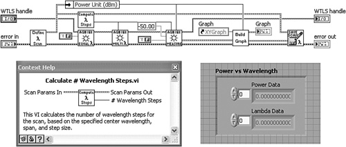
The optical filter measurement routine propagates the wavelength and power data arrays using two separate wires. As shown on the right half of Figure 4-6A, the two wires are used together in most places, with the exception of Convert Power Units VI, which requires only the power data. In Figure 4-6B, the Convert Power Units VI is incorporated as a subVI within Measure VI. Hence, the power data is converted to appropriate units before it is returned. Also, the wavelength and power arrays are modularized into a cluster. Finally, the routine that unbundles several scan parameters and calculates the number of wavelength steps has been modularized into a cohesive subVI.

Figure 4-6A. Two separate wires for the wavelength and power arrays are used together in most places and may be modularized into a cluster. The routine for calculating the number of wavelength steps can be modularized into a subVI. The routine for converting power units can be performed within Measure VI.

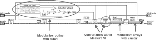
Figure 4-6B. The routine is further modularized with Calculate # Wavelength Steps VI and Power vs. Wavelength cluster.

I cannot overemphasize this rule. (Consequently, it is further discussed in Chapter 6, “Data Structures.”) Save every cluster as a type definition or strict type definition. A type definition (or typedef, for short) is a control that maintains its data type information in a CTL file. The typedef is copied onto any number of VI panels as a control or indicator, or diagrams as a constant, by either dragging and dropping from the project tree, or choosing either Select a Control from the Controls palette or Select a VI from the Functions palette. All instances of the typedef maintain the data type specified in the typedef’s CTL file. Therefore, multiple instances of the control are maintained from one location via the Control Editor window. This is extremely beneficial for clusters because most clusters are used in multiple places, and the contents are subject to change. For example, in Figure 4-5C, new parameters are added to or removed from the Wavelength Scan Params cluster by simply adding or removing the corresponding controls to the typedef. In Figure 4-5D, all of the subVIs containing the typedef will automatically update to match the revised cluster.

A strict type definition (also known as strict typedef) maintains the control’s properties, in addition to the data type, in the CTL file, so that all instances of the strict typedef maintain an identical appearance and behavior. I prefer the strict typedef because I often find that I need to maintain a common range, default value, and appearance among instances. To specify the type definition status, choose the corresponding item from the Typedef Status ring control on the Control Editor window’s toolbar. Clusters and type definitions are discussed in greater detail in Chapter 6.

4.3 Data Flow

This section covers data flow, the fundamental principle of LabVIEW. It contains a brief review of basic principles and style rules, considerations regarding variables and Sequence structures, and techniques for optimizing data flow. The rules are illustrated with a combination of simple diagram snippets and a working application example.

4.3.1 Data Flow Basics

In LabVIEW, data flows along wires from source terminals to destination terminals. A block diagram node executes when data is received at all wired input terminals. Upon completion, data is supplied to its output terminals and propagates to the next node in the dataflow path. The dataflow principle distinguishes LabVIEW from traditional text-based software-development environments. The following are some basic rules regarding data flow.

With only one exception, always flow data through wires running from left to right. This is a sacred, age-old convention within the LabVIEW community. However, Feedback Nodes and Sequence Locals are built-in LabVIEW constructs that inherently violate this rule. In my opinion, the Feedback Node is a credible exception when the length of the right-to-left wire segment is very short, resulting in a reduction of wire clutter compared to a shift register. Sequence Locals are relevant only to Stacked Sequence structures, which should be avoided.

Zooming in on the diagram of Spaghetti VI, discussed in Chapter 1, we observe several violations of the left-to-right dataflow rule, including the wires highlighted in Figure 4-7. We also see unnecessary bends and kinks (4.11), overlapping wires and nodes (4.15), multiple local variables (4.17), and many other issues contributing to the spaghetti effect.

Figure 4-7. The diagram of Spaghetti VI contains several wires that violate the left-to-right dataflow rule.

Left-to-right data flow is accomplished by first positioning the order-dependent nodes from left to right so that interconnecting wires naturally flow left to right. In most cases, the order of execution is determined by data dependency. Simply propagate one or more common data elements, such as the error cluster, between the functions that require a specific execution order. This is similar to what is illustrated in Figure 4-4.

Coercions are the unattractive dots that appear on terminals when there is a numeric representation mismatch. By default, they are colored gray prior to version 8.2, and red subsequent to version 8.2, but you can specify their color by selecting Tools»Options; choose Colors from the Category list, deselect use default colors, and click on the color next to Coercion Dots. Coercions indicate that LabVIEW is converting the data from one type to another. It is an additional operation that requires additional memory to store each representation. Eliminate coercions when possible, particularly with larger data structures such as arrays and clusters. Techniques for maintaining similar data types to prevent coercions are discussed in Chapter 6. Keep your eyes open for coercion dots, and try to eliminate them.

One simple way to avoid coercions and save development time as well is to create controls, indicators, and constants from a node’s terminals on the diagram. This is accomplished by right-clicking on the desired node’s connector terminal and selecting Create»<Control/Indicator/Constant> from the context menu. The corresponding control, indicator, or constant is automatically created, having the data type that matches the terminal it is wired to. Additionally, the wiring assignment is completed and the item inherits the label of the node’s terminal. Hence, several editing steps are completed from just one menu selection.

Dots at wire junctions have no functional purpose except for drawing attention to wire junctions. They are larger and usually more prevalent than coercion dots. During the development of a dense diagram, they help distinguish junctions from overlapping wires. However, they can mildly interfere with identifying coercion dots. Also, if you generally avoid overlapping wires, it is not necessary to highlight junctions. My personal opinion is that dots at wire junctions appear a tad obnoxious on a diagram with clear wiring and efficient data flow. Because wire junctions can be identified by triple-clicking on a wire of interest, I recommend disabling dots at wire junctions. This selection is available from Tools»Options; select Block Diagram from the Category list and deselect Show dots at wire junctions.

Avoid using Sequence structures, unless they are required. In particular, never use a Sequence structure to force the execution order of functions that can execute in parallel. This is a common tendency of former text-based programmers that are accustomed to textual statements executing in the order in which they appear. Challenge yourself to avoid Sequence structures. Instead, try to keep independent functions and routines parallel to each other. For example, the Flat Sequence shown in Figure 4-8A is unnecessary. Additionally, the variables are unnecessary. The diagram shown in Figure 4-8B is functionally equivalent but cleaner and more efficient. Specific rules on the practical and impractical use of Sequence structures and variables are discussed in the sections that follow.

Figure 4-8A. This Flat Sequence structure is unnecessary because the contents need not execute sequentially.

Figure 4-8B. The Sequence structure is replaced with parallel nodes, which LabVIEW executes efficiently.

Nesting is the placement of structures within structures. Nesting beyond two or three layers begins to obscure the underlying logic and data flow, as shown in the Nested VI example from Chapter 1. It is difficult to visualize all of the possible logical branches and data paths in a highly nested diagram. Excessive nesting is normally caused by faulty logic, excessive use of Sequence structures, and lack of standard design patterns. Faulty logic is an important concern because the more nesting, the more difficult it is to comprehend the diagram to identify and debug the problem. Spend some time creating a flow chart, truth table, or Karnaugh map to understand the desired logic before implementing the source code. In Chapter 8, specific architectures that minimize nesting are presented. However, some level of nesting is required even for the most common and useful design patterns. Because the structures that comprise the design pattern are recognized as the design pattern, they need not count toward the excessive nesting layers. In this case, always save the VI with the most important frames of the nested structures selected so that the diagram opens this way by default. The most important frame is either the most frequently executed logical branch or the frame that reveals the most nodes. Finally, note that maximizing data flow and minimizing Sequence structures goes a long way toward preventing excessive nesting.

4.3.2 Practical Variables and Sequence Structures

Throughout this book, I generally recommend avoiding local and global variables and Sequence structures because they undermine dataflow principles. Now let us take a moment to consider their practical applications. In some circumstances, they serve important and useful purposes.

Write local variables are the best method for writing to controls from the diagram. This is necessary to programmatically initialize control values, such as configuration parameters that are read from file. Also, local and global variables represent a fast and easy method of sharing data between parallel processes such as continuous loops or VIs. However, read local and global variables have no inputs, and write local and global variables have no outputs. Therefore, the execution order of a sequence containing local and global variables cannot be specified using data flow. Property Nodes and Shared Variable nodes have error terminals and are viable dataflow alternatives to local and global variables. A Property Node configured to read or write a control’s Value property is similar to a local variable, but it causes the diagram to switch to the user interface thread to read or write the value directly from the front panel, in a synchronous manner. Local variables read or write from the control’s terminal on the block diagram, which does not trigger an immediate thread change and user interface update. A single process shared variable functions similarly to a global variable that performs error checking. Local and global variables are generally simpler and more efficient than Property Nodes and Shared Variable nodes. If you must use local and global variables and you must specify the order in which they are written or read, then you must use a Sequence structure.

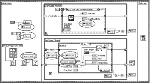
Use a Sequence structure to specify execution order when a specific order is required and no data dependency exists. Specifically, Sequence structures can order initialization routines, including write variable operations, to ensure that they are performed at the very beginning of the application. Likewise, Sequence structures can force shutdown routines, such as Quit LabVIEW, to occur at the very end of the application. Figure 4-9 illustrates an example of a diagram that utilizes an initialization routine, two parallel loops, and a shutdown routine. The application’s primary purpose is to run a test involving a lengthy data acquisition process upon user command via the Run Test Boolean control. Because the data acquisition process is lengthy, the application is divided into separate parallel master and slave loops, including an Event Loop for processing user interface events, and a DAQ Loop for performing the data acquisition task. The Event Loop is the master that triggers the data acquisition task within the slave DAQ Loop. The parallel loops enable the user interface to remain responsive while the data acquisition task runs in the background. LabVIEW spawns separate execution threads for each parallel loop.

A local variable is used to initialize the Sensor Scaling cluster with values read from file. Global variables are used to share Boolean data between parallel loops. The Acquire global variable triggers the data acquisition task from the Event Loop. The Stop global variable stops the DAQ Loop when the Event Loop stops, and vice versa. The application has a Boolean control that writes to the Stop global from within the Event structure’s Quit Value Change event case, not shown. Specifically, when either loop stops, it passes a Boolean TRUE value through a While Loop tunnel to a Stop write global variable. Upon the next iteration, the other loop reads this value from its corresponding Stop read global variable, and stops. Global variables require less configuration and effort than alternative constructs such as shared variables, occurrences, notifiers, and queues. If one simple and unambiguous data item is being written, with only one or two instances of a write global variable and on only one occasion throughout the application, the global variable is a good choice. It is unnecessary to set up a shared variable, occurrence, notifier, or queue for such a limited scope.

In Figure 4-9A, two single-frame Sequence structures are placed on each side of the While Loops, and wires are used to create data dependency between each structure. The large Sequence structure on the left initializes the variables and passes two wires out of tunnels to the While Loops. Because data will not pass through the tunnels of the Sequence structure until all its operations have completed, via the principle of data flow, the write local variable operations must occur before the data propagates through the tunnels. Because the While Loops receive data from the initialization Sequence structure, the While Loops cannot begin executing until the initialization Sequence structure has fully completed. This condition is known as data dependency. Notice also that the Boolean data that is passed to the border of the Event Loop is not actually used within the loop. Instead, the wire terminates on the While Loop’s border. Nonetheless, this wire ensures that the Event Loop begins executing only after the initial Sequence structure completes. This is known as artificial data dependency.

Figure 4-9A. Two single-frame Sequence structures are used for forcing the execution order of the Initialization routine, two While Loops, and Shutdown routine.

The Shutdown routine consists of a Sequence structure on the right containing the Quit LabVIEW function. It receives data from the two parallel loops, ensuring that the Shutdown routine executes last. Also note that the General Error Handler VI propagates the error cluster as an input from the DAQ Loop and an output to the Shutdown Sequence structure. This forces the General Error Handler VI to execute after the DAQ Loop stops, but before the Shutdown Sequence structure can begin. The diagrams in Figure 4-9B and Figure 4-9C are functionally equivalent to the diagram from Figure 4-9A, except that they utilize three-frame Stacked and Flat Sequence structures, respectively. Stacked Sequence structures are less desirable than Flat Sequence structures because only one frame is visible at a time, they require sequence local terminal for data flow between frames, and the multiple frames hide the data flow. Flat Sequence structures facilitate data flow between frames using tunnels, and all frames are simultaneously visible. Also, each frame of a Flat Sequence structure has a uniform appearance and does not require artificial data dependency. Therefore, the Flat Sequence implementation in Figure 4-9C is preferred in this example.

Figure 4-9B. A Stacked Sequence structure requires sequence local terminals to pass data between frames.

Figure 4-9C. A three-frame Flat Sequence structure facilitates data flow between frames via wires and tunnels, and all frames are visible. This is the preferred implementation.

4.3.3 Impractical Variables and Sequence Structures

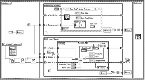
Most local and global variables and Sequence structures used in practice are not necessary. Most often, they are overused by developers who have not learned efficient dataflow principles. The best way to master data flow is to force oneself to avoid variables and Sequence structures unless absolutely required. Indeed, mastering data flow is synonymous with minimizing variables and Sequence structures. In fact, even the example in Figure 4-9 has more efficient dataflow implementations. Figure 4-10A is a copy of Figure 4-9C with several unnecessary local and global variables circled. The Acquire global variable triggers the data acquisition task from the Run Test Value Change event case within the Event Loop. The DAQ Loop monitors the Acquire global variable until its value becomes TRUE and then executes the data acquisition task within the True frame of the Case structure.

Figure 4-10A. Avoid polling variables in loops, such as the Acquire read global variable in the DAQ Loop. Additionally, the Sensor Scaling local variables can be replaced by a wire, and the Curve local variable is unnecessary.

Polling is the condition in which a loop continuously monitors a resource until it reaches a specific value or state. Never poll a variable within a loop. In Figure 4-10A, the DAQ Loop executes at top speed, inefficiently utilizing the processor to detect a change in value of the Acquire global variable. Instead, use a synchronization construct, such as an occurrence, notifier, or queue. These functions allow the slave loop to sleep until the synchronization construct fires an event. Another observation from Figure 4-10A is that the Sensor Scaling write and read local variables can be replaced by a wire. The write local variable might still be useful if the Sensor Scaling data read from file needs to be displayed in a control. However, the read local variable inside the DAQ Loop is unnecessary. Finally, the Curve local variable is not necessary because it initializes a graph indicator to its default value, which is already the control’s state when the VI loads into memory.

In Figure 4-10B, the Acquire global variable is replaced with an occurrence, the Curve local variable is eliminated, and the Sensor Scaling local variables are replaced by a wire. The occurrence allows the DAQ Loop to sleep, not utilizing the processor, until the Set Occurrence function executes inside the Event Loop or a timeout occurs. The timeout input terminal of the Event Loop’s Event Structure and the DAQ Loop’s Wait on Occurrence function is set to 200ms, allowing each loop to periodically poll the Stop global variable and update the stop condition. Polling the Stop global every 200ms is more efficient than polling the Acquire global at full speed, but it is still a violation of Rule 4.33.

Figure 4-10B. An occurrence is used in place of the Acquire global variables, a wire replaces the Sensor Scaling local variables, and the Curve local variable is eliminated.

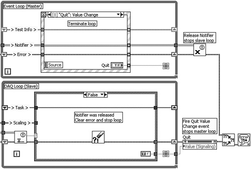
Applying a notifier instead of an occurrence further streamlines data flow and efficiency, as observed in Figure 4-11. A notifier is a synchronization construct that is similar to an occurrence. However, a notifier is programmatically released, causing the Wait on Notification to return from an indefinite wait. By comparison, the Wait on Occurrence function cannot terminate programmatically. Also, the notifier sends data from the sender to the receiver. In Figure 4-11A, the Event Loop’s Run Test event case calls the Send Notification function along with a Boolean TRUE instructing the DAQ Loop to acquire data. The DAQ Loop’s Wait on Notification function wakes up and returns the TRUE value from the notification output terminal to the case selector, and the Acquire routine runs. When any event fires that causes the Event Loop to stop, the Release Notifier function is called outside the Event Loop. For example, if the user clicks the Quit Boolean control, the Quit Value Change event case of the Event Loop fires, as shown in Figure 4-11B. This causes the Event Loop to stop, and the Release Notifier function runs. The DAQ Loop’s Wait on Notification function immediately wakes up and returns a FALSE value from the notification output terminal, and an error from the error out terminal. The DAQ Loop executes the Case structure’s False case, which clears the error and stops the loop. Hence, the Event Loop fully controls the DAQ Loop, without variables. Also, notice that an error in either loop stops both loops, without variables. Specifically, the error status is unbundled and wired to each loop’s conditional terminal. A TRUE error status in the Event Loop stops the loop and calls the Release Notifier function, terminating the DAQ Loop as previously described. Additionally, a TRUE error status in the DAQ Loop terminates the loop, and the Property Node outside the DAQ Loop runs. This Property Node is associated with the Quit Boolean control and is configured to set the Quit Value Signaling property, which fires a Quit Value Change event within the Event Loop. The Quit Value Change event case runs and stops the Event Loop. Consequently, variable polling is no longer necessary, and all instances of the Stop global variable are eliminated. This implementation optimizes the master/slave synchronization efficiency, as shown in Figure 4-11B.

Figure 4-11A. A notifier replaces the occurrence, and the Stop global variables are eliminated. This implementation optimizes the synchronization efficienctly.

Figure 4-11B. The Quit Value Change event case stops the loop. The Release Notifier function is called outside the loop, causing the Wait on Notification function in the DAQ Loop to wake up and return an error. The error is cleared in the False case, and the DAQ Loop terminates.

4.3.4 Optimizing Data Flow

As discussed, mastering LabVIEW’s dataflow principles is synonymous with eliminating local and global variables and Sequence structures, when feasible. The previous sections identify the practical and impractical uses of these programming constructs. This section presents alternatives that optimize data flow, including shift registers and looped Case structures.

Shift registers are terminals on looping structure borders that shift data between loop iterations. They are functionally and conceptually similar to terminals that extend wires from the end of one loop iteration to the beginning of the next. Shift registers are viable alternatives to local and global variables when the required scope of data sharing is limited to a single While Loop, Timed Loop, or For Loop. Unlike variables, shift registers do not create copies of their data when read and are maximally efficient.

To avoid wire clutter and maintain organization, space most shift registers tightly, and group them near the top of the loop. This creates a data highway that is limited to an area near the top of the loop and minimizes wire crossovers. Leave just enough space between the shift registers to apply free labels on each wire near the left terminals. Exceptions to shift register grouping include error clusters and case selectors. Error clusters normally enter and exit near the bottom of loops. Also, case selectors are frequently positioned near the middle. Therefore, error clusters and case selectors are usually kept separate from the data highway at the top.

A looped Case structure is a Case structure embedded within a loop. It functions similarly to a Stacked Sequence structure when the sequentially ordered code is placed in cases of the Case structure instead of the frames of the Sequence structure. However, the execution order of the cases is controlled programmatically via the Case structure’s selector terminal. This is more flexible than a Sequence structure, for which the execution order is strictly determined by the frame numbers. Use shift registers on the loop to share data between cases of the looped Case structure. Shift registers promote better data flow than the Sequence Locals of a Sequence structure because the data enters and exits the cases in a consistent location and the data flows left-to-right.

Figure 4-12 provides four different implementations of a test sequence comprised of 12 sequentially ordered test VIs. Each test VI shares several common inputs and outputs, including a DAQmx task, a cluster of sensor scaling coefficients, a cluster of high and low test limits, and an error cluster. Additionally, each test appends a row to the Test Results table indicator for reporting the test results. These updates are performed immediately after each test is completed. Also, the limits for each test are calculated within the previous test VI, based on its test results.

Figure 4-12A utilizes a Stacked Sequence structure, in violation of Rules 4.27 and 4.32. The error cluster is passed between frames using sequence local terminals on the Sequence structure’s inner border. Because sequence local terminals can be written to only once, 11 terminals are required to propagate the error cluster among 12 frames. This clutters the appearance and causes wiring and dataflow rules violations. Most frames contain one right-to-left data flow and a wire crossover caused by reading from a sequence local terminal on the right border or writing to a sequence local terminal on the left border. Additionally, the Stacked Sequence structure implementation contains 48 local variables. These include two local variables per frame for updating the Test Results table indicator, plus two local variables per frame for reading and writing the test limits.

Figure 4-12A. A test sequence is implemented using a 12-frame Stacked Sequence structure. It contains 48 local variables plus 11 sequence local terminals, and right-to-left data flow.

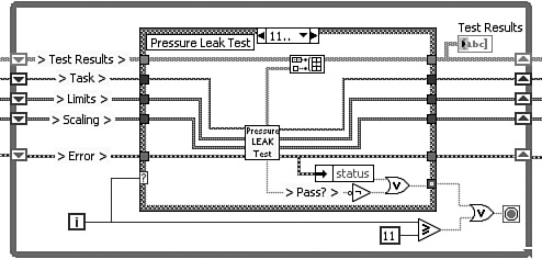
Figure 4-12B utilizes a looped Case structure using a For Loop as the looping structure. The code within the cases of the Case structure is functionally equivalent to the code within the frames of the Stacked Sequence structure from the prior implementation. However, only five shift registers are required to replace 48 local variables and 11 sequence local terminals used by the Sequence structure implementation. The wiring is clear, with no right-to-left data flow or wire crossovers. Figure 4-12C contains a looped Case structure that utilizes a While Loop instead of a For Loop. This implementation is similar to the For Loop, with one important distinction: The While Loop is programmed to terminate if a test fails or an error occurs, without completing the full test sequence.

Figure 4-12B. The test sequence is implemented using a looped Case structure with a For Loop as the looping structure. Five shift registers replace the local variables and sequence local terminals.

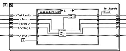
Figure 4-12C. An alternate looped Case structure utilizes a While Loop that terminates the test sequence if a test fails or an error occurs.

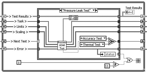
A looped Case structure need not be limited to sequentially ordered execution of numerically selected cases. A flexible sequencer utilizing the Classic State Machine design pattern is shown in Figure 4-12D. The Classic State Machine, discussed extensively in Chapter 8, consists of a looped Case structure with an enumerated data type for the case selector and a shift register for passing the next case selection between loop iterations. The cases are intuitively labeled based on the text items of the enumerated data type instead of integers. This eliminates the free labels within each case. Also, the Classic State Machine programmatically selects the next case, based on an operation performed in the previous case. In this manner, the test sequence is formed dynamically. This implementation maximizes flexibility compared to the previous implementations.

Figure 4-12D. A flexible sequencer is implemented utilizing the Classic State Machine design pattern. An enumerated data type and shift register are utilized for the case selection. The sequence is formed dynamically.

Let us now apply the flexible sequencer to a larger application. Consider the master/slave test VI from Figure 4-11. The slave loop is modified to perform the sequence of 12 tests from Figure 4-12 instead of the single data acquisition task. On the surface, it appears as though the test sequence should be placed inside the existing Case structure, resulting in four layers of nesting, a violation of Rule 4.28. However, the slave loop itself can be modified into a flexible sequencer. Specifically, in Figure 4-13A, the slave loop has been converted into a Queued State Machine design pattern, for which a queue replaces the notifier for synchronization and messaging between loops, an enumerated data type replaces the Boolean case selector, and the Case structure contains multiple cases corresponding to the tests. The queue is similar to a first-in, first-out buffer that stores multiple enumerations representing the slave loop’s case selections or states. As shown in Figure 4-13A, the master loop’s Run Test event case calls the Enqueue Element function in a For Loop, enqueuing the 12 cases that comprise the test sequence. Additionally, in Figure 4-13B, notice that the File I/O functions that read the Sensor Scaling data from file appear within the Initialize case of the slave loop’s Case structure. The Enqueue Element function to the left of the slave loop enqueues the Initialize case via an enumerated constant, which ensures that the Initialize case executes first. Therefore, the functionality of the Queued State Machine is not limited to the test sequence, but also performs initialization and other routines as required. This implementation is neater and more flexible than the notifier implementation from Figure 4-11.

Figure 4-13A. The master/slave application from Figure 4-11 is modified to execute the 12-step test sequence from Figure 4-12, utilizing the Queued State Machine design pattern for the slave loop.

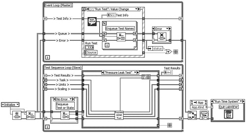
Figure 4-13B. The functionality of the Queued State Machine design pattern is expanded to accommodate an initialization routine in addition to the test sequence. The Initialize case contains the File I/O functions that read the scaling data.

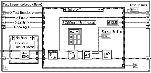
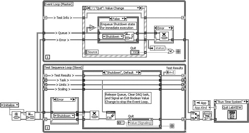
Figure 4-13C illustrates how the loops stop each other in the event of a user interface event or error. If the user presses the Quit Boolean control, the Quit Value Change event case adds the Shutdown state to the front of the queue via the Enqueue Element at Opposite End function. This causes the Test Sequence Loop to run the Shutdown state and terminate the loop. If an error occurs in the Event Loop, the Error case of the Case structure releases the Queue, causing the Dequeue Element function in the Test Sequence Loop to return with an error and execute the Shutdown state, since it is the Case structure’s Default case. Finally, if an error occurs in the Test Sequence Loop, it calls the Shutdown state which releases the Queue, clears a DAQ task, and fires the Quit Value Change event, causing the Event Loop to terminate. The Queued State Machine design pattern is described in greater detail in Chapter 8.

Figure 4-13C. The loops stop each other if the Quit Value Change event occurs in the Event Loop, or an error occurs in either loop.

4.4 Examples

In this section, a variety of block diagram examples are presented, both good and bad. Let us begin with the bad and gradually transition to the good. The bad examples are particularly effective at illustrating the reason for many of the block diagram style rules presented thus far.

4.4.1 SubVI from Selection

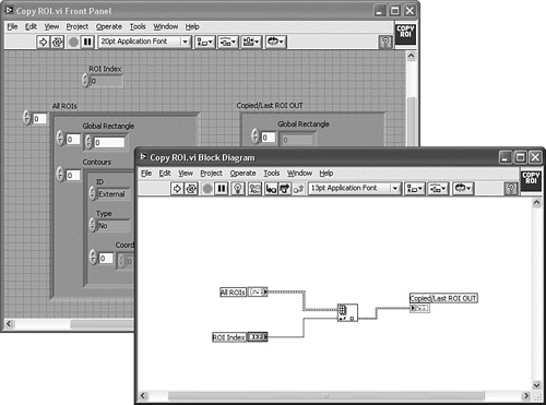
As observed in Chapter 3, “Front Panel Style,” the SubVI from Selection utility is the world’s most flagrant style violator. This is the process of selecting an area of the diagram and choosing Edit» Create SubVI. The worst possible programming practice is to create a subVI from selection and not clean up the aftermath. The terminal locations and labels, wiring, connector assignments, icon, and description all require corrective action. Sometimes the resulting subVI diagrams appear as if a bomb went off inside them. SubVIs created using this tool never conform to good style, and rework is mandatory.

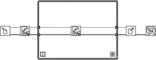
Figure 4-14A corresponds to the diagram of the SubVI from Selection VI front panel example presented in Chapter 3. It contains several telltale signs of a subVI from selection. The wiring is kinked, the objects are tightly spaced, and the control labels are nonsensical. For example, the task ID and error control terminals are improperly labeled task ID out and error out. Additionally, one of the indicators has the generic label Numeric. What is curious is that the subVI has a custom icon and description, and the control terminals are within reasonable proximity to the structure. Perhaps it was partially repaired. The wiring and terminal labels have been cleaned up in Figure 4-14B. Also, Figure 4-14C contains equivalent code using the waveform data type and the newer sound output VIs released with LabVIEW 8. This is the preferred implementation.

Figure 4-14A. This diagram is the product of the SubVI from Selection utility, without the mandatory repairs.

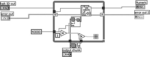
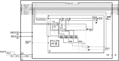
Figure 4-14B. The VI is revised to incorporate appropriate control labels, object spacing, and clear wiring.

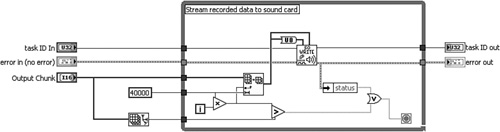
Figure 4-14C. The VI is rewritten to utilize the waveform data type and LabVIEW 8 sound VIs.

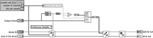
Layout: The diagram (4-14A) is small and the objects are poorly spaced.

Modularity: Not applicable because there are only a few nodes. However, the VI itself is the outcome of the developer’s attempt to modularize the calling application.

Wiring Scheme: The wires are excessively kinked, a common byproduct of the subVI from selection utility. Additionally, one wire is not lined up with the tunnel in which it enters the loop.

Data flow: Data flows vertically as well as horizontally, including through two tunnels on the bottom border of the While Loop. Also, there is one coercion dot as sound data is converted from I16 to U8.

4.4.2 Excessively Nested VI

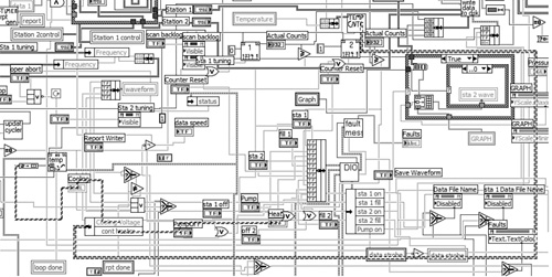
The diagram of Excessively Nested VI, shown in Figure 4-15, is oversized and severely nested. The top illustration is the Navigation window, which, unfortunately, is the only way to view the whole diagram. The bottom illustration is a highly nested section of the diagram. Less than half of the overall diagram is visible on the screen with 1280×1024 resolution. Navigation entails much scrolling and even more flipping through the frames and cases of the nested structures. The quadrant shown contains 11 layers of nesting. It is not possible for even the most advanced developers (and blackjack players) to comprehend all the logical branches represented. Avoid large diagrams and avoid excessive nesting. Chapter 8 presents standard diagram architectures that help prevent large and unwieldy diagrams like this one.

Figure 4-15. The Navigation window shown at the top is required to navigate the oversized diagram. The subsection at the bottom magnifies 9 of the diagram’s 11 layers of nesting.

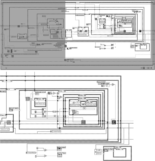
Layout: The diagram is oversized, overly nested, and unwieldy.

Modularity: There are only 40 user VIs out of 2,040 nodes, for a modularity index of just 1.9. Hence, it is not modular.

Wiring Scheme: There are many long wires due to a large diagram, along with several unnecessary bends.

Data flow: Nesting obscures data flow. There are several instances of right-to-left data flow, as well as data entering structures through vertical tunnels.

4.4.3 Haphazard VI

The diagram of Haphazard VI, shown in Figure 4-16, contains haphazard wiring and data flow. More wires enter and exit structures vertically than horizontally. There are many wire bends and kinks. Data is flowing left to right, right to left, up, down, and all around. Additionally, several local variables are improperly initialized outside the While Loop in parallel with code that is reading the values from the corresponding control terminals inside the loop. Because there is no data dependency between the initialization operations and the While Loop, the order of execution is not specified. Therefore, these controls may not be correctly initialized before they are accessed within the looping structure. This is a situation in which a single-frame Sequence structure with artificial data dependency—or a multiframe Flat Sequence structure—is required, similar to Figures 4-9A and 4-9C, respectively. The unusual icon convention is another matter that is discussed in Chapter 5.

Figure 4-16. This diagram has excessive wire bends, haphazard data flow, and unusual icon convention. The order of execution between the local variable write operations and the While Loop is not specified.

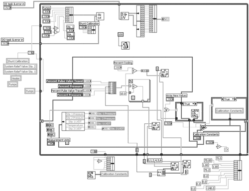
Layout: The diagram is sized appropriately, with medium to low density.

Modularity: There are 13 user VIs out of 396 nodes, for a modularity index of 3.3. Clutter outside of the loop should be combined into one initialization subVI.

Wiring Scheme: Wires contain excessive bends and kinks. Many wires enter and exit structures vertically. Several wires are too long.

Data flow: Data flows in all directions. Initialization routines are not explicitly ordered to execute before the main While Loop. There are excessive coercions.

4.4.4 Right to Left VI

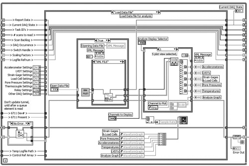
Right to Left VI is an application that acquires waveform data from pressure and volume transducers until an event occurs, and then logs the last sample of each waveform to a comma-delimited text file. It is illustrated in Figure 4-17. The diagram utilizes efficient data flow, and contains liberal comments. However, it contains one wire that is routed right to left, as shown near the center of the primary Case structure’s Log Data case. The wire is cleverly labeled to indicate the right-to-left data flow. On the surface, it appears to represent good right-to-left data flow style. In a pinch, one neatly labeled right-to-left wire never hurt anyone. However, it is still right-to-left nonetheless, a rule violation.

Figure 4-17. Right to Left VI is a top-level VI containing low-level functions for forming the file path, a local variable, a vertical tunnel, and right-to-left data flow.

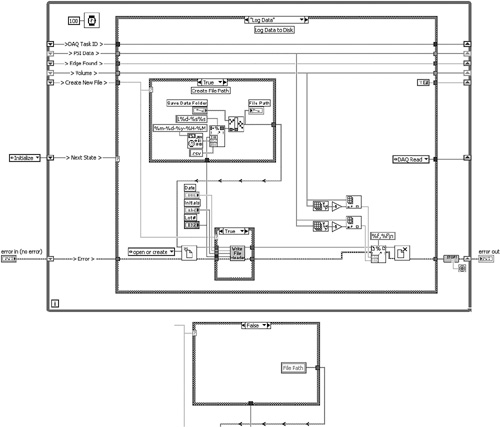
Close inspection reveals that the right-to-left wire is a file path that is formed by some low-level functions within an inner Case structure. Whenever a collection of low-level functions that work together to perform a cohesive routine appears on the diagram of a high-level VI, it is a good opportunity for a subVI, as per Rule 4.7. Additionally, the Case structure’s False case contains a read local variable for the File Path indicator. This represents an opportunity for a shift register to replace a variable. Finally, a wire is routed from the Lot # control terminal vertically through a tunnel in the inner Case structure’s bottom border. This violates Rule 4.13. Hence, one right-to-left-flowing wire leads us to four style rule violations.

• Layout: This is a sparsely populated Classic State Machine design pattern, which is discussed in Chapter 8.

• Modularity: This application is relatively simple, containing only 6 user VIs and 173 nodes, for a modularity index of 3.5. As seen in the Log Data case, low-level functions for file path forming should be modularized into a subVI, as per Rule 4.7.

• Wiring Scheme: Wires are straight and some overlapping is required.

• Data flow: Most data flows left to right, with the exception of one wire that flows right to left. Shift registers are utilized to maintain data between loop iterations. The File Path local variable can be replaced with another shift register.

4.4.5 Left to Right VI

Figure 4-18 shows the same VI from Figure 4-17, formerly known as Right to Left VI, modified with several enhancements. It contains a subVI for forming the file path, and a shift register for maintaining the file path between loop iterations. The revised diagram no longer requires the local variable, tunnel on the bottom border, or right-to-left data flow. Additionally, the object spacing and structure sizes have been reduced, providing a higher overall object density. An important lesson learned in this example is that the style rules are interrelated. The more you follow on a consistent basis, the easier it becomes to maintain good style throughout an application.

Figure 4-18. Left to Right VI is functionally equivalent to Right to Left VI but contains multiple style enhancements.

Layout: This is the Classic State Machine design pattern with high object density.

Modularity: Additional subVI increases the modularity index to 4.0.

Wiring Scheme: Wires are straight and some overlapping is required.

Data flow: All data flows left to right. An additional shift register maintains the file path value between loop iterations.

4.4.6 Centrifuge DAQ VI

The diagram of Centrifuge DAQ VI shown in Figure 4-19 is neat, intuitive, and very well documented. The primary data elements are read from shift registers and wired through tunnels into the primary Case structure, facilitating good data flow. Each wire is labeled outside the Case structure and then bent upward to create additional space within the Case structure. Near the bottom of the diagram, an array of control references is passed to a subVI for manipulating properties. The Queued State Machine design pattern is readily expandable via adding cases to the primary Case structure and items to the enumerated data type that is wired to its selector. More features of this application are discussed in Chapters 6 and 8.

Figure 4-19. Centrifuge DAQ VI contains many advanced features, including control references and the Queued State Machine design pattern.

Layout: This diagram actually has two parallel While Loops, only one of which is visible on the monitor and included in this illustration. It utilizes the Queued State Machine design pattern.

Modularity: There are 113 user VIs out of 2,887 nodes, for a modularity index of 3.9. SubVIs are used for manipulating control properties, reducing real estate occupied by Property Nodes.

Wiring Scheme: Clusters are utilized to avoid wire clutter. Wire bends create additional space within the main Case structure.

Data flow: Data flows strictly from left to right. Queues are used to pass data between parallel loops without variables. Shift registers are used over variables wherever feasible. The application contains 50 variables, primarily used to initialize control values.

4.4.7 Screw Inspection VI

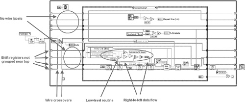
The Screw Inspection VI diagram shown in Figure 4-20A is clear, with a staircase dataflow appeal. It is modular with a particularly attractive icon convention that is featured in Chapter 5. At first glance, the layout, wiring, and data flow look pretty good. Shift registers are utilized over variables, maximizing data flow. Wires and objects are evenly spaced. However, close inspection reveals multiple rules violations, as shown in Figure 4-20B. These include unnecessary wire bends and kinks (4.11), overlapping objects (4.15), unlabeled long wires (4.18) including wires exiting shift registers (4.37), right-to-left data flow (4.22), discontinuous error clusters (4.23), and coercion dots (4.24). There is unnecessary clutter, including constants and labels to the left of the shift registers. The constants are unnecessary because they are the same as the default values for each shift register’s data type when first loaded into memory. Error handling is functionally nonexistent. Figure 4-20C contains the same VI with multiple improvements. However, the error cluster propagation is deferred until Chapter 7, “Error Handling.”

Figure 4-20A. Screw Inspection VI is neat, with cute icons and a staircase wiring appeal. At first glance, it appears to have satisfactory layout, wiring, and data flow.

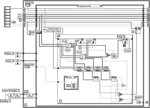
Figure 4-20B. Close inspection reveals multiple violations of the block diagram style rules.

Figure 4-20C. Multiple improvements are made to the VI. Error cluster propagation is discussed in Chapter 7.

• Layout: The diagrams in Figures 4-20A and 4-20B are sufficiently dense and occupy less than one screen. One overlapping label exists.

• Modularity: There are 7 user VIs out of 292 nodes, for a modularity index of 2.4.

• Wiring Scheme: Wiring appears neat overall. Clusters help minimize clutter. However, there are unnecessary bends and kinks, overlapping objects, and unlabeled long wires, including wires exiting shift registers.

• Data flow: Most data flows like a staircase, from left to right and top to bottom. Shift registers minimize variables. However, error handling is discontinuous and some right-to-left data flow exists.

4.4.8 Optical Filter Test VI

The optical filter test application introduced in Section 4.2.2 is continued in Figure 4-21. This illustration represents the top-level VI that calls the filter measurement routine as a state within the Queued State Machine design pattern. Specifically, the filter measurement routine from Figure 4-6A is incorporated in the Normal Sweep case of the state machine in Figure 4-21A. The application’s execution order is controlled programmatically using the queue. Shift registers facilitate data flow. However, the shift registers are randomly spaced (4.36) and not labeled (4.37). This results in wires flowing through the middle of each state, dividing the diagram into multiple sections. Additionally, there are multiple data flow and wiring rules violations, including wire crossovers (4.15) and right-to-left data flow (4.22). Specifically, the error cluster crosses over several shift register wires to reach the Dequeue Element function on the left of the Case structure. Also, the low-level routine that calculates the number of wavelength steps propagates the result to two instrument driver VIs below it. Finally, readability is hindered by several low-level routines on a high-level VI (4.7), in addition to the data flow and wiring issues.

Figure 4-21A. The optical filter test application contains a Queued State Machine design pattern. The shift registers are not grouped, the wires exiting the shift registers are not labeled, there is right-to-left data flow, and there is clutter from low-level routines.

In Figure 4-21B, the shift registers are labeled and grouped near the top, forming a nonintrusive data highway and increasing the space available for nodes in each of the Case structure’s cases. The queue functions are moved to the bottom of the diagram, eliminating crossovers of the error cluster wire. A subVI replaces the low-level routine for computing the number of wavelength steps, reducing clutter and eliminating the right-to-left data flow. Additionally, the wavelength and power data are modularized into clusters. Consequently, the diagram of Figure 4-21B is much more readable than the one in Figure 4-21A.

Figure 4-21B. The shift registers are grouped near the top, the wires exiting the left shift register terminals are labeled, wire crossovers are reduced, the array size computation is modularized into a subVI, the power and wavelength arrays are modularized into a cluster, and right-to-left data flow is eliminated.

Endnotes

¹ NI’s Developer Zone contains a Code Sharing area and an Instrument Driver Network containing free downloads, including drivers for more than 5,000 instruments. The URL is www.ni.com/devzone/.