Chapter 6. Data Structures

The data structures of an application consist of LabVIEW’s built-in data types and developer-defined data constructs. Data types are the fundamental data elements depicted by unique terminal or wire styles on the diagram. Data types define the memory size and functionality of the data. Data constructs are data sets that use the fundamental data types as elements, such as arrays and clusters. Data structures are the data types and data constructs used by an application. Data structures are defined by the developer’s choice of controls, arrays, and clusters on the VI front panels, as well as the operations performed on the diagrams.

Control types determine how users understand and operate the front panels. This includes both GUI VIs that users interact with and subVIs that only the developers see. As presented in Chapter 3, “Front Panel Style,” judicious selections for controls make the panels intuitive, user-friendly, and reliable. Additionally, each control type supports one or a limited set of data types. Consequently, the developer’s choice of controls helps determine the application’s data structures.

Data constructs are used to organize data and reduce wire clutter on the diagram. Consistent use of data constructs throughout an application help make it easy to understand and maintain, as well as memory efficient. Nested data structures have special considerations with respect to performance and memory use, as discussed later in this chapter.

It is a fact common to all modern software that execution speed is inversely proportional to memory use. Specifically, memory and data storage access rates are the principal performance barriers of modern computing devices. A LabVIEW application’s memory use is defined by its data structures and the operations performed on the data. LabVIEW does not impose restrictions on the data structures that an application may use. Therefore, an application’s performance is directly related to the developer’s choice of data structures and corresponding operations. This chapter presents style rules for choosing data structures that provide intuitive, reliable, and efficient operation.

6.1 Data Structure Design Methodology

Evaluate the data structures during the design phase of application development. Describe the data required for each major subsystem, including the GUI, data acquisition and instrument I/O, analysis, report generation, file I/O, database queries, and network and interapplication communications. Examine all of the application’s primary data sources and destinations. Prototyping front panel development is a very useful technique for specifying the GUI, as discussed in Chapter 2, “Prepare for Good Style.” Additionally, use prototype front panels to specify the data required for each component of the application.

When coding begins, the data structures are implicitly declared by the developer’s choice of controls and indicators on the front panels, as well as the inputs and outputs required by the nodes on the diagrams. Implementing the data structures for a VI is generally a three-step process. First, select the controls and data types. Second, configure the properties of those controls. Third, group the controls into data constructs, if appropriate. In this section, we start with some general rules to guide us through this process. The sections that follow discuss rules that apply to specific types of LabVIEW data structures.

6.1.1 Choose the Controls and Data Types

The term simple has several connotations with respect to LabVIEW controls and data structures. Simple data structures store data in contiguous memory addresses. They include all scalar data types, such as Boolean, numeric, and string; arrays of Boolean and numeric, and clusters containing only the aforementioned simple data types. Simple controls are controls that are intuitive and easy to operate, and that represent simple data structures. Simple controls possess properties that can be configured to help validate user and programmatic input. When properly configured, simple controls are reliable and memory efficient.

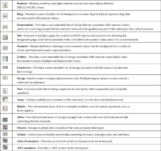
To some degree, control types can be classified in order of operational and data simplicity. For example, numeric controls are very intuitive, can be configured to restrict values to a specified range, and are stored efficiently in memory according to the representation. String controls can contain any alphanumeric data, without restriction, and are stored as blocks of contiguous bytes, 1 byte per character. Boolean controls are maximally restrictive, allowing only a value of TRUE or FALSE, and are stored as byte integers. Therefore, of these three control types, Boolean is the simplest, followed by numeric and then string. Table 6-1 contains the complete list of LabVIEW control types, listed in approximate order of operational and data simplicity. The controls at the top are the simplest, beginning with Boolean and numerics, and the controls at the bottom are potentially the most complex. Note that the list is both overlapping and subjective. For example, numeric simplicity depends on the representation. Arrays and clusters are data constructs, and their simplicity depends on their contents. Also, a string’s memory use is the same as a one-dimensional array of byte integers of equivalent length. Therefore, the control types are approximately organized by data simplicity. Because arrays have the potential to contain larger and more complex data than strings, the string type is ordered simpler than array.

Table 6-1. LabVIEW Controls and Descriptions, Listed in Top-Down Order of Operational and Data Simplicity

Because many of the control types can be configured to represent or contain a variety of data types, memory efficiency depends on the combination of the control type and data type. Therefore, it is useful to consider data type efficiency in addition to control type simplicity. Specifically, the data types define the size and simplicity of the data in memory. For example, we can organize the numeric data types in order of representation, for which the smallest integer representation is the most memory-efficient data type and the largest floating-point representation is the least efficient. Table 6-2 contains the complete list of LabVIEW data types, presented in approximate order of memory efficiency. As shown, the smallest numeric representation is an 8-bit (1-byte) integer, and the largest is an 8- to 16-byte extended-precision floating-point numeric.

Table 6-2. LabVIEW Data Types and Descriptions, Listed in Top-Down Order of Memory Efficiency

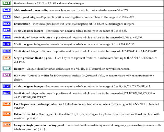
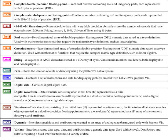
Similar to the list of control types in Table 6-1, the order of data types in Table 6-2 is approximate and overlapping. For example, an enumeration consists of two components, an unsigned integer and a set of string labels. The efficiency of the unsigned integer component depends on its representation, either 8-bit, 16-bit, or 32-bit. The efficiency of the string component depends on the quantity and lengths of the labels. These properties are configured by the developer. Likewise, the more complicated data types listed near the bottom of the table, such as Dynamic and Variant, depend on the data and attributes they contain.

Choose the control types and data types for intuitive operation and memory efficiency. Table 6-3 presents a matrix containing the control types and supported data types. The control types are organized along the top horizontal heading in left-to-right order of operational and data simplicity, similar to Table 6-1 turned sideways. The data types are listed along the left vertical heading in top-down order of memory efficiency, similar to Table 6-2. The cells of the table indicate the compatibility of each control type with each data type. Use this table to optimize the control and data type selections in order of operational simplicity and memory efficiency. Consider the type of data that is required, and choose the control type that is best suited to represent that data. Begin on the top left, and evaluate each control type from left to right. If your data element has two selections that are opposites, choose a Boolean control. If you need to provide a range of numeric selections, first consider a ring or an enumeration, followed by a numeric. Select the first control type that meets the operational requirements. Next, traverse the corresponding column of data type compatibility, from top to bottom, until you identify the first data type that provides the desired functionality. The result is the control and data type combination that provide the simplest operation and greatest memory efficiency.

Figure 6-3. The Simplicity and Compatibility of Each Control Type Listed in the Top Horizontal Heading with Data Types Listed in the Left Vertical Heading

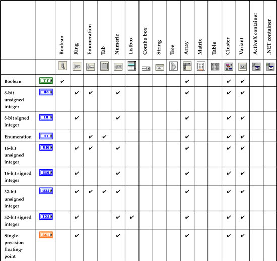
Note that the use of Rules 6.1 and 6.2, and Table 6-3 help prevent the application from generating invalid data. For example, you would never choose a string control for data that is strictly numeric. A numeric control is much easier and more reliable for a user to operate, and the data is stored efficiently. Also, if you have a discrete number of alphanumeric selections, use an enumeration or a ring control before using a string control. As we can see from Table 6-3, enumeration and ring controls are much simpler than string controls because they restrict user input to a limited number of discrete selections and are represented as integers.

Finally, note that enumeration and variant appear in each table as both controls and data types. This is because they are both. An enumeration is a special data type consisting of a numeric with associated text strings. A variant is a self-describing data type that encodes any LabVIEW data into a generic format. Similarly, arrays and clusters can be considered data types as well as controls. However, the data type of arrays and clusters is undefined until they are populated with specific data structures. Unlike enumerations and variants, wiring assignments cannot be made from the terminals on the diagram until the data type definition is completed by depositing controls into the array and cluster shells. Otherwise, any wires are broken. Therefore, arrays and clusters do not become valid data types until populated.

Referencing Theorem 6-1, the most important consideration in choosing controls and data types is consistency. Dissimilar data types require conversions, either explicitly via the formatting and conversion functions or automatically via coercions that appear as dots on terminals. LabVIEW allocates separate memory buffers to store each representation of data. Therefore, dissimilar data types lead to extra programming, processing, buffer allocations, and memory consumption. Good LabVIEW developers strive to optimize the performance and memory use in their applications.¹ Consistent data types reduce the level of programming effort required, while ensuring efficient and reliable performance.

Rules 6.1, 6.2, and 6.3 must be considered together when developing an application’s data structures. Controls that are simple to operate, data types that are memory efficient, and overall consistent data structures are desired. How do we ensure that each consideration is satisfied? Carefully examine the data requirements of each component or subVI, and choose data types that are intuitive, efficient, and consistent. When compromises between memory efficiency (6.2) and data structure consistency (6.3) are required, always choose consistency (6.3). Per Theorem 6-1, memory access time is the universal latency. The more memory operations are performed by our applications, such as buffer allocations, the greater the negative impact is on performance. All data type conversions entail buffer allocations that are susceptible to this issue. However, larger data types, such as DBL instead of I16, do not necessarily affect the number of memory buffer allocations. Indeed, allocating a 4,096 element array of DBL may require the same memory access time as allocating a similar array of I16. Rather, allocating an array of I16 and later converting to an array of DBL entails multiple buffer allocations.

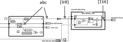
Consider the example in Figure 6-1. An instrument driver for an oscilloscope acquires and processes a waveform through a hierarchy of subVIs, as shown in Figure 6-1A. The lowest-level VI is Get Raw I16 Waveform VI, shown in Figure 6-1B. This VI reads the raw data as a binary string, converts the data to an array of unsigned byte integers, combines every two successive integers into a single 16-bit signed integer, and returns the raw data as an array of 16-bit signed integers. Because there are normally 2 bytes per sample, 16-bit signed integer is the simplest and most memory efficient numeric data type for representing this data, per Table 6-3.

Figure 6-1A. A section of the VI Hierarchy window for a top-level VI that calls an instrument driver to acquire a waveform from an oscilloscope. The instrument driver uses a call chain of three subVIs, including read, fetch, and get.

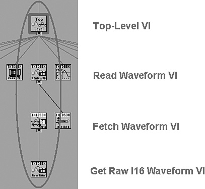
Figure 6-1B. Get Raw I16 Waveform VI returns an array of 16-bit signed integers. This is the most memory efficient data type for storing the waveform in this VI.

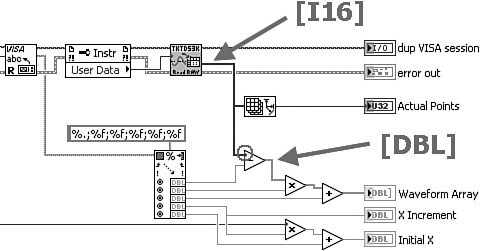
In Figure 6-1C, Fetch Waveform VI converts the raw data returned from Get Raw Waveform VI into a scaled array via several arithmetic functions. Because the offsets and scaling factors are double-precision floating-point numeric, the array of raw data must be coerced to double-precision floating-point numeric prior to the mathematical operations. This is indicated by the coercion dot on the subtract function. The coercion creates a new buffer of data, expanded to 8 bytes per array element, in addition to the previous buffer. Hence, the coercion increases the memory use by a factor of 4, in addition to allocating a new memory buffer.

Figure 6-1C. Fetch Waveform VI scales the raw array to a scaled array of double-precision floating-point numbers. Arithmetic operations between dissimilar data types cause a coercion, which allocates a new memory buffer.

Next, the scaled array passes through Read Waveform VI without modification, as shown in Figure 6-1D. Finally, the top-level VI, shown in Figure 6-1E, bundles the scaled array together with the Initial X and X Increment and updates the Waveform Graph. The bundle function causes the scaled array to be copied into the cluster that it builds, thus forming an additional memory buffer.

Figure 6-1D. Read Waveform VI passes the scaled array without modification.

Figure 6-1E. The top-level VI bundles the scaled array and other waveform components into a cluster and updates a waveform graph.

Each VI in this call chain has different data requirements, and the control and data types have been chosen for maximum simplicity and memory efficiency within each specific VI. However, the dissimilar data types in this call chain increase the memory consumption by a factor of 9 versus the original array of 16-bit signed integers. More important, the waveform’s data type is converted five times throughout the call chain, adding unnecessary buffer allocations that reduce execution speed. Therefore, using the simplest and most memory efficient data types within each individual VI reduces the overall performance of the application because of the inconsistent data structures.

Figure 6-2 contains the same example, except consistent data types are used throughout the call chain. In Figure 6-2A, every 2 successive bytes of the binary string are converted directly to an array of double-precision floating-point numbers. Note that this selection requires four times more memory than the 16-bit signed integer used in Figure 6-1A, but it improves consistency throughout the call chain. Also notice that the intermediate conversion of the binary string to 8-bit unsigned integers has been eliminated, partially offsetting some of the extra memory and processing required for the conversion to double-precision floating-point numbers. In Figure 6-2B, the raw array is scaled using arithmetic operations applied to consistent data types, eliminating the coercion and extra memory buffer versus Figure 6-1B. Also, a waveform data type is assembled. In Figure 6-2C, the waveform passes through Read Waveform VI without modification. Finally, in Figure 6-2D, the waveform passes up to the top-level VI and updates the waveform graph without modification.

Figure 6-2A. Get Raw DBL Waveform VI returns an array of double-precision floating-point numbers, which compromises memory efficiency within this VI for data structure consistency throughout the application. Also, an intermediate conversion is eliminated.

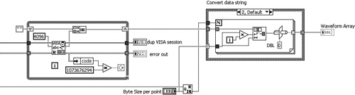
Figure 6-2B. Fetch Waveform VI performs arithmetic operations using similar data types, avoiding the coercion, and constructs a waveform data type.

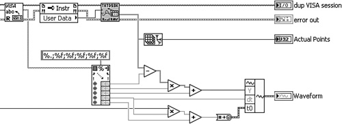
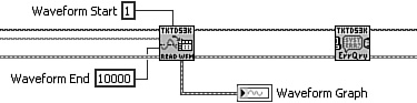
Figure 6-2C. Read Waveform VI passes the waveform without modification.

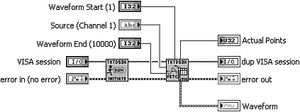
Figure 6-2D. The top-level VI simply updates the waveform graph. No modifications to the data are required.

In this example, consistent data types modestly reduce memory consumption, while substantially reducing the number of buffer allocations. Hence, overall performance is optimized. Additionally, the waveform data type is a convenient data structure that requires fewer terminals and wires for the multiple VIs of the call chain. When the waveform data type is formed, the developer can use the high-level VIs on the Waveform palette to perform common waveform operations. Hence, Rules 6.1, 6.2, and 6.3 have been combined for best overall performance.

It should be noted that, in some applications, the raw waveform is preferred in the smallest format instead of either waveform data type or double-precision floating-point numbers. For example, if the objective is to acquire and stream the raw data to file, the smallest file size and fastest disk streaming rate are desired. In this instance, streaming the raw binary data to file in the format that it is read directly from the instrument provides the optimum result. Be sure to log the waveform scaling information to convert the data to the desired engineering unit offline.

6.1.2 Configure the Properties

After the controls have been selected, the next step is to configure their properties. For Boolean command buttons, it is common to configure the Mechanical Action and Boolean Text properties. For numeric controls, configure the format, precision, and range. For strings, specify the display style, single line, and wrap behavior. Customize the appearance and default value properties of each control, or define your own custom controls using the Control Editor.

To help promote proper VI use, configure appropriate default values for each control. Consider the common use cases, determine what typical value each control may utilize, and configure it as default if it exists. At the very least, the VI should be able to load from memory and run properly without modifying the control values. Required inputs such as refnums and instrument sessions are an exception. For subVIs, indicate the default value in parentheses at the end of the owned label so that it is visible from the panel as well as the Context Help window of the calling VI.

As discussed in Chapter 3, intuitive and succinct owned labels help document the controls and indicators. Additionally, enter one or two sentences for each control description that further describes the control’s purpose, default value, and range, unless it is completely intuitive based on the label. Control descriptions provide documentation that is visible from the Context Help window. In Chapter 9, “Documentation,” we discuss how a documentation set is generated containing the control labels and descriptions. It behooves us to enter the description, even if it seems unnecessary, or we might be disappointed when a formal document is required.

A strict type definition is a control that is customized and saved as Strict Type Def. in the Control Editor window. The Control Editor forms a CTL file that maintains the data type and properties of the strict type definition. This allows the multiple instances to maintain the same customized properties, including appearance and behavior. The properties are then modified via the Control Editor, and changes are automatically applied to all instances. Strict type definitions are discussed in detail in Section 3.4.2, “Consistency.” In general, if the control has one or more properties that have been configured and will have more than one instance requiring the same properties, save it as a strict type definition.

6.1.3 Create the Data Constructs

After the controls and properties are specified from the previous two steps, the final step is to implement the data constructs. This is primarily accomplished by grouping related controls into arrays and clusters, and saving as type definitions. Arrays are multivalued data sets of the same type. Clusters combine multiple controls of any type into a new data structure. Arrays and clusters are represented by a single terminal and wire on the diagram. They are very useful for organizing data and reducing subVI terminals and wire clutter.

Consider the Torque Hysteresis VI shown in Figure 6-3. First, the application prompts the user to enter some information about the unit under test (UUT). The application queries a database, and if the UUT is recognized, it prompts the user to enter a set of motion control parameters. Next, the VI runs a test consisting of a motion profile that acquires torque versus angle data. Upon test completion, the VI performs a statistical analysis to the data and generates a report. Finally, the application saves the data to file. Following the guidelines in Chapter 4, “Block Diagram,” these requirements are implemented using a modular diagram containing separate subVIs for each task, as follows: UUT Information Dialog (1), Motion Parameters Dialog (2), Run Test VI (3), Compute Statistics VI (4), Generate Report VI (5), and Save Data VI (6). A simplified version of the top-level diagram containing these six subVIs is shown in Figure 6-3A, prior to the assignment of data structures. The data that is generated by the first four subVIs and processed by the latter two subVIs is shown in Figure 6-3B.

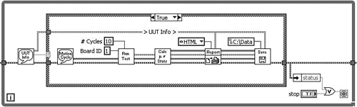
Figure 6-3A. Top-level diagram of Torque Hysteresis VI, prior to assignment of data constructs

Figure 6-3B. Data generated by the first four subVIs and processed by Generate Report VI and Save Data VI

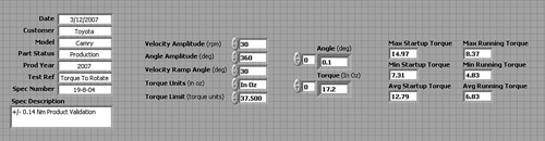
Figure 6-4A shows the diagram of Torque Hysteresis VI implemented without clusters. Many wires and terminals are required to pass the data from the first three subVIs to the successive subVIs. The subsequent subVI, Compute Statistics VI, generates six additional calculated values that are used by Generate Report VI and Save Data VI. However, the latter two subVIs do not have enough terminals to receive this data using wires, despite the use of the connector pattern with the maximum 28 terminals, as shown in Figure 6-4B. Instead, global variables are used to pass the excess data between subVI diagrams. Additionally, maintenance of this VI is a chore. If an additional parameter is added to the UUT Information Dialog, corresponding controls, terminal assignments, and wires must be added to three subVIs, or new global variables are required.

Figure 6-4A. Top-level diagram of Torque Hysteresis VI implemented without clusters. The wire and subVI terminal density complicates maintenance.

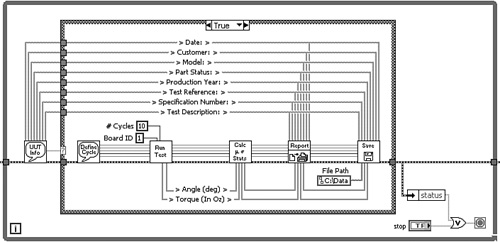
Figure 6-4B. Although Generate Report VI has the connector pattern containing the maximum 28 terminals, it is not sufficient for the six additional values calculated in Compute Statistics VI.

Applying Rule 6.7, the data from Figure 6-3B is grouped into the clusters shown in Figure 6-5A. The diagram of Torque Hysteresis VI is implemented using clusters, as shown in Figure 6-5B. Specifically, the eight parameters of UUT information are bundled into a cluster named UUT Information. Five motion control parameters are stored in a cluster named Motion Parameters. The Motion Parameters cluster is passed to Run Test VI. Upon test completion, the VI stores the raw data acquired during the test into a cluster named Torque vs Angle. Next, the Motion Parameters and Torque vs Angle clusters are both passed to Compute Statistics VI. The computed results are stored into a cluster named Statistics. Also, Compute Statistics VI passes the Motion Parameters and Torque vs Angle clusters unmodified to Generate Report VI. This VI receives the UUT Information cluster from the UUT Information Dialog and creates the report. Finally, all clusters are passed to Save Data VI, where the data is saved to disk.

Figure 6-5A. The 21 parameters from Figure 6-3B are grouped into four clusters.

Figure 6-5B. Top-level diagram of Torque Hysteresis VI is implemented using clusters. The diagram appears neat and orderly, and maintenance is simplified.

In this example, 21 parameters have been logically grouped into four clusters. All data is passed among subVIs using terminals and wires. All subVIs use the standard 4×2×2×4 connector pattern. The diagram appears neat and orderly due to the use of clusters. Each cluster is saved as a type definition, for ease of maintenance. It is simple to add and remove parameters by adding and removing controls to the type definitions.

The sections that follow contain more guidelines for simple data types and simple and complicated data constructs, as well as many more examples.

6.2 Simple Data Types

Simple data types are a subset of the fundamental LabVIEW data types that are stored in contiguous memory locations. They include Boolean, numeric, string, path, picture, and several special numeric types. In this section, we consider style rules pertaining to the simple data types.

6.2.1 Boolean

Boolean is the simplest control type in terms of both operational and data simplicity and has two possible values, TRUE or FALSE. Boolean data is actually stored as a byte integer. Hence, the Boolean data type is really no more efficient in terms of memory size than the smallest integer representation. However, Boolean controls are extremely intuitive. They have two clearly defined states and resemble objects commonly seen in everyday life. They include push buttons, toggle switches, command buttons, slide switches, LEDs, and radio buttons.

The most important rule with Booleans is to use them to represent parameters that have exactly two states that are logical opposites—for example, On or Off, Yes or No, Open or Closed, and Stop or Go. When the two states are not opposites, use a text ring or enumeration to provide text selections that more accurately describe the choices.

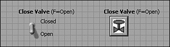
When a parameter’s states are indeed opposites, it becomes easy to assign the control a name that clearly identifies its behavior in relation to the TRUE and FALSE Boolean states. For example, if we have a control named Valve State, the TRUE/FALSE behavior is unclear. Instead, consider a name such as Close Valve. In this case, we can determine from the name that the valve is closed when TRUE and open when FALSE. Per Rule 3.23, always enter the default value in parentheses for subVIs. This eliminates any chance of ambiguity. In the latter example, we have Close Valve (F = Open).

Use command buttons to represent Booleans that invoke immediate action on GUI VI panels, such as Trigger, Run, Cancel, Quit, and Close Valve. Simply start with the OK, Cancel, or Stop button from the Boolean Controls palette, and customize it for your needs. This may involve simply changing the Boolean text or editing the size, fonts, and colors as well. Do not use command buttons for settings that do not generate immediate action, such as configuration properties. Instead, use the control that appears most intuitive for the users. NI’s Instrument Driver Guidelines² recommends the vertical slide switch for all Boolean controls within an instrument driver. Most applications can be completed using just two types of Boolean controls: command buttons for action on GUI VI panels, and vertical slide switches for configuration parameters.

Always label the TRUE and FALSE states of toggle and slide switches with names corresponding to the behavior of each state, and position the labels next to the physical switch positions. Specifically, from the control’s shortcut menu, choose Advanced»Customize to open the Control Editor window. Drop free labels adjacent to each of the control’s switch positions and enter the text describing the TRUE and FALSE states. Edit the font, positions, and orientations of the labels so that they line up with the TRUE and FALSE switch positions. Close the Control Editor window and apply the custom changes. This method makes the label a permanent part of the control that you cannot accidentally move or delete while editing the VI. A faster alternative is to display the control’s Boolean text. Boolean text is made visible by selecting Visible Items»Boolean Text from the control’s shortcut menu, and it can be repositioned and edited. However, the Boolean text shows only one state at a time and is not as intuitive as the TRUE and FALSE state labels.

Figure 6-6 provides a vertical toggle switch and command button for a valve control configured with three different labeling schemes. The command button contains a glyph of a valve imported as a decal. In Figure 6-6A, the Valve State control labels are ambiguous in terms of the TRUE/FALSE behavior. In Figure 6-6B, the Close Valve control labels clearly depict the TRUE/FALSE behavior. Additionally, the vertical toggle switch contains visible Boolean text with default ON/OFF strings. In Figure 6-6C, the Boolean text of the vertical toggle switch has been replaced with more intuitive state position labels identifying the TRUE/FALSE behavior as Closed and Open. Additionally, the default value for each control has been appended to the control labels in parentheses. This additional text is distracting on a GUI VI but is helpful for reinforcing a subVI terminal’s behavior via the Context Help window. Per Rule 6.10, the command button is preferred for controls that invoke immediate action, such as opening and closing an important valve. However, proper labeling makes the two control types approximately equivalent.

Figure 6-6A. Two alternatives for valve control include the vertical toggle switch and the command button with valve image decal. The label Valve State is ambiguous in this example.

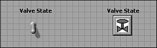
Figure 6-6B. The owned label Close Valve clearly identifies the TRUE and FALSE behavior. The vertical switch has Boolean text visible with default TRUE/FALSE state labels. The command button is preferred for a GUI VI.

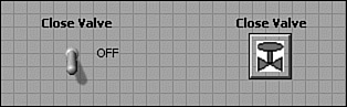
Figure 6-6C. The TRUE and FALSE states of the vertical toggle switch are appropriately labeled Closed and Open. The default value of each control is identified within the labels using parentheses.

LabVIEW’s front panel objects have a useful property whereby any control can be converted to an indicator, and vice versa. In some instances, this does not make sense. For example, buttons and switches should not be used as indicators, and LEDs should not be used as controls. These reversed associations are counterintuitive and might confuse people, thereby violating Rule 6.1.

Boolean controls that are part of a cluster maintain the same appearance when the cluster is used as both control and indicator. In this case, it is difficult to avoid violating Rule 6.12 because consistent data structures are desired, per Rule 6.3. There are two alternatives. First, a command button can be customized to neutralize its appearance, similar to the status control of the error cluster. This is the preferred approach. Alternatively, separate clusters can be created for controls, containing the buttons or switches, and indicators, containing the LEDs. In this case, coercions will result if the clusters are saved as type definitions and then wired together. Because clusters are often saved as type definitions, this approach violates Rule 6.3 and should be avoided.

6.2.2 Numeric

Two categories of numeric data types exist: integer and floating-point number. Integers are used to represent whole numbers, while floating-point numbers are required for fractional data.

Section 6.1.1, “Choose the Controls and Data Types,” discusses the significance of simplicity, memory efficiency, and data type consistency. Per Rule 6.3, it is important to maintain consistent data structures throughout an application. In most situations, use 4-byte signed integer (I32) representation for integer data types, and 8-byte double precision (DBL) representation for floating-point numbers. Anything with physical units, such as voltage, power, frequency, length, angle, and similar quantities, should be DBL.

LabVIEW’s numeric functions can accept and operate on any numeric data types. Polymorphism is a term that describes a function or VI with one or more terminals that can accept more than one data type. Polymorphic functions and VIs adapt to the input data type instead of breaking the wire or forcing a coercion to occur on the input terminal. More important, the function completes its operation successfully. Most of LabVIEW’s built-in functions, VIs, and constructs that are not polymorphic consistently use I32 for integers and DBL for floating-point data. For example, the iteration and count terminals of looping structures are I32, as are the index terminals of array and string manipulation functions. DAQmx and most instrument driver VIs return DBL, or waveforms containing arrays of DBL. Likewise, the analysis VIs process arrays of DBL. Therefore, using I32 for integer and DBL for floating-point numbers helps maintain consistent data types throughout an application and avoids unnecessary coercions and conversions.

For completeness, two exceptions to this standard include digital pattern I/O and traditional data acquisition VIs. Reading or writing digital pattern data from a data acquisition device generally requires 1- or 4-byte unsigned integers (U8, U32). Also, the analog traditional DAQ VIs use 4-byte single-precision (SGL) numeric, if configured to read or write scaled data instead of waveforms. However, the DAQmx VIs and driver are both functionally and stylistically superior to the traditional DAQ VIs and driver. I highly recommend upgrading any legacy applications that use traditional DAQ.

If you are like me, you may have wondered why LabVIEW uses I32 for unsigned quantities such as loop iteration and count terminals, versus U32. The LabVIEW inventors intended I32 and DBL to be the prominent data types for integers and fractional numbers, respectively. Therefore, LabVIEW uses I32 and DBL to help promote their use.

By default, LabVIEW formats floating-point numbers within numeric controls and indicators automatically. Specifically, LabVIEW displays the appropriate number of decimals, and switches between decimal and exponential notation, similar to a hand-held calculator. Sometimes it is desirable to display a specific number of decimal places all the time, to indicate the precision of a physical measurement, coefficient, or other parameter. Unless you have a good reason such as this, use the automatic formatting.

Numeric controls with integer representation are formatted as decimal data, by default. Hexadecimal, Octal, and Binary formats can also be selected from the Format and Precision tab of the Numeric Properties Dialog. Select Advanced Editing Mode to make the Numeric Format Codes visible. When configuring numeric controls to represent data in these less common formats, always make the control’s radix visible. This is done by selecting Visible Items»Radix from the shortcut menu. If the radix is not visible, the data is generally assumed to be decimal format.

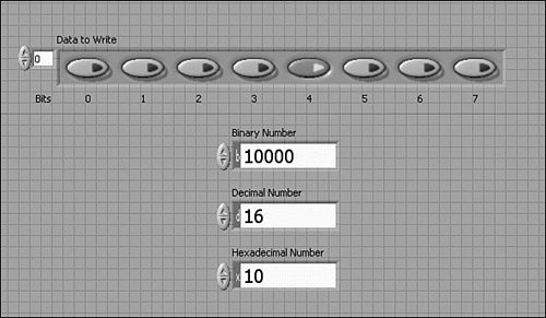
Figure 6-7 shows four different controls that may be used to write a digital pattern to an 8-bit digital I/O port. They include an array of Boolean and three numeric controls configured for binary, decimal, and hexadecimal notation, respectively. Although each control represents the same value, the different formats for each numeric control would be interpreted much differently without a visible radix.

Figure 6-7. Four different controls contain a digital pattern for writing to an 8-bit digital I/O port. They include an array of Boolean, and three numeric controls formatted as binary, decimal, and hexadecimal. It is important to make the radix visible for numeric controls not configured for decimal notation.

6.2.3 Special Numeric

Four numeric data types that have special properties are the time stamp, reference number (refnum) and I/O name, text and menu rings (ring), and enumeration (enum). The time stamp data type stores absolute time with separate 8-byte fields for seconds and fractions of a second. Hence, the time stamp is extremely precise. Refnums and I/O names are references to a specific instance of an open resource, such as a file, instrument or device, network connection, image, LabVIEW application, VI, or control. They function similarly to a pointer to a data structure describing the resource. While the purpose of the two types of references is similar, the controls are substantially different. Specifically, I/O names display a value in an intuitive format, whereas refnums do not. VISA, IVI, and DAQmx Name Controls, for example, provide information about the specific hardware that they reference. ActiveX and .NET Refnums provide only a data type in a label. Because each type of resource has different requirements, the actual data type, memory use, and underlying data structure is different for each. The placement of refnums and I/O names in Tables 6-2 and 6-3, which list the data types ordered according to memory efficiency, only considers the reference portion of these data structures. It is important to note that this is not representative of the actual resource.

The ring and enum controls map text selections to numeric values. They are very useful for presenting a discrete number of selections that are intuitively described using text labels on the front panel, but the numeric is more functional on the diagram. Enum controls are always represented as unsigned integers, and the text selections are mapped to sequential numbers starting with 0. Ring controls may have any numeric representation, and the text selections are mapped to any value within the range allowed by the representation, including nonsequential, negative, and floating-point numeric values. The advantage of using enum and ring controls on the panel is that text selections can be more descriptive and meaningful than numbers, and selecting one item from a discrete list is very intuitive for the user. These controls play an important part in good programming style because they promote readability on both the front panel and the diagram.

On the diagram, enum and ring constants can display the text labels instead of or in addition to the numeric values they represent. Specifically, create a constant from the shortcut menu of a ring or enum terminal by selecting Create»Constant from the terminal’s shortcut menu. The constant contains a pick list of the control’s text selections, similar to the control on the panel. You can choose any of the text selections and show or hide the digital display. Additionally, when an enum is wired to the selector terminal of a Case structure, the text selections appear in the Case structure’s selector area. This is why the enum is used for the State Machine design patterns discussed in Chapter 8, “Design Patterns.”

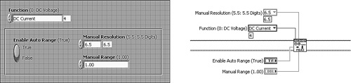
Figure 6-8 shows an example of an instrument driver subVI that configures a digital multimeter. In Figure 6-8A, numeric controls are used to configure the Function and Manual Resolution parameters on the subVI’s front panel. These parameters are programmed through terminals on the subVI’s connector pane. The subVI call shown to the right uses numeric constants to configure these parameters. The value of 4 for Function is meaningless, and the value of 6.5 for Manual Resolution is risky. Specifically, the range of valid selections and the meaning of each selection is not very clear. In Figure 6-8B, text ring controls are used in place of the numeric controls. The subVI call contains text ring constants that were created from the terminals’ context menus. These constants contain a discrete number of text labels that clearly describe each selection and limit the user to valid choices. Hence, the text rings are more functional, intuitive, and reliable than the numeric controls.

Figure 6-8A. The front panel of an instrument driver subVI contains numeric controls for programming the measurement function and resolution. The subVI call uses numeric constants for specifying these values, which are not meaningful and prone to error.

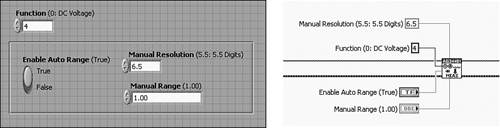
Figure 6-8B. The instrument driver subVI panel contains text ring controls instead of numeric controls. Constants created from the terminals’ shortcut menus provide pull-down lists containing a discrete number of intuitively labeled choices.

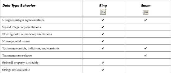
The text selections for enums and rings form a very important source of documentation on the panel and diagram that is built into these controls. I recommend enums over rings for maximum readability, including the case selector text. However, there are a few exceptions where a ring control must be used over an enum. Use a ring control when the text labels map to nonsequential, negative, or fractional values, or if localization is an issue. Also, use a ring control when creating an instrument driver or developer toolset intended for international distribution. The text embedded within an enum uniquely defines its data in the native language of the LabVIEW version in which it is created. The enum functions correctly when ported to localized versions, but the language of the enum text is not translated. For this reason, the NI Instrument Driver Development Guidelines recommends text ring controls and Booleans over enums. The text within the text ring gracefully ports to the localized language because the text is a symbolic mapping to the integer. Finally, the Strings[] property is read and write programmable for a ring but is readable and not writeable for an enum. A comparison between the enum and ring is summarized in Table 6-4.

Table 6-4. A Functional Comparison Between Ring and Enum Data Types

It is common to add and remove items from the enum controls many times during application development and maintenance. However, any clones you copy or constants you create do not maintain the same items as the original control after cloning, unless the original control is saved as a type definition. This is easy to overlook and a common source of misbehavior. Therefore, always save your enum controls and as type definitions. This is accomplished by choosing Advanced»Customize from the control’s shortcut menu, select Type Def. or Strict Type Def. in the Type Def. Status ring of the Control Editor window, and save the control to a CTL file. Per Rule 6.6, choose the Strict Type Def. if the control has custom properties in addition to the text labels, and choose the Type Def. otherwise. Constants as well as controls that are formed from a type definition maintain an association so that when the type definition’s items are edited, all instances are automatically updated as well. Note that a ring control must be saved as a strict type definition in order to provide similar behavior.

6.2.4 String, Path, and Picture

String, path, and picture are variable length data types stored in contiguous memory. String controls provide tremendous flexibility for entering or passing alphanumeric data. However, they lack filters or built-in methods to restrict the format, number of characters, case, or spelling of the data. Therefore, they provide the greatest opportunity for error.

Avoid string controls on GUI VI panels except where free-form alphanumeric data is required. As developers, we should never trust the user to enter data in a specific manner, and the more invalid ...options we provide the user, the less reliable our software is. As per Theorem 3.1, reliability is the developer’s responsibility.

Two useful applications of string controls and indicators include entering descriptions and displaying instrument responses. If an operator needs the capability to enter free-form comments, such as a description of a one-of-a-kind test, or the cause of an alarm limit violation, a string control is appropriate. Instead of having a string control on the main GUI VI panel, create a dialog VI that prompts the user for the description and closes immediately afterward.

String indicators are invaluable for troubleshooting instrument communications. Instrument control is performed at a low level using calls to VISA Write and VISA Read. These functions write instrument commands and read responses as strings. Instrument drivers provide a layer of abstraction between the developer and the command and response strings, which are generally cryptic. However, when developing or troubleshooting an instrument driver, it is usually necessary to view these low-level messages in string indicators. Indeed, string indicators have some very useful display modes, including backslash () and hex. In backslash mode, we can view nondisplayable characters such as tabs, carriage returns, and line feeds via their backslash codes, such as , , and . In hex mode, we can view binary data in hexadecimal format.

Use Table 6-1 to locate simpler alternatives to string controls. For example, enums and rings provide a discrete set of alphanumeric choices, as previously described. Always use path controls for entering or programming alphanumeric data representing a file path. LabVIEW formats the path using the standard syntax for the host’s operating system. This ensures platform portability. The Browse button makes it simple for a user to interactively navigate and select a directory or file path, and should be kept visible on GUI panels. Configure the Browse Options, including Selection Mode, to restrict the user’s choices and validate the data.

The picture data type stores a sequence of operation codes and data for drawing an image in a picture indicator. Operation codes are low-level instructions that tell the CPU what to draw. There are about 50 operation codes representing a wide variety of geometrical shapes and bitmap configurations. The data are the operands for each operation code. They include coordinates, colors, and other operation-specific data. The operation codes and data stored by the picture data type are transparent to the developer. Use the Picture VIs on the Picture Functions palette to create the pictures. Because the picture data type is stored in contiguous memory, it is a relatively simple data type, similar to string and numeric arrays.

6.3 Data Constructs

Data constructs are collections of one or more of the fundamental data types used to form a new data type. They include developer-defined constructs such as array, cluster, variant, variable, and queue, as well as built-in data types such as matrix, error, waveform, and dynamic. Arrays and clusters provide tremendous flexibility and utility, and are the primary means for organizing data in an application. This section presents style rules for data constructs, with emphasis on arrays and clusters.

6.3.1 Simple Arrays and Clusters

Array and cluster controls consist of shells or containers within which any data type or construct may be placed. The complexity of arrays and clusters depends entirely on their contents. This could be as simple as a single scalar Boolean or as complex as nested arrays and clusters. This section discusses simple arrays and clusters.

Arrays store data sets that have multiple values of the same data type. In memory, arrays consist of a heading containing the length of each dimension stored as 4-byte signed integers, followed by the data that comprises the array. Arrays containing one of the simple data types described in Section 6.2, “Simple Data Types,” store the heading and data together in contiguous memory locations.

Most references consider arrays as collections of related data, very similar to clusters, except that the data elements have the same type. Indeed, this is correct. However, there are very important distinctions between arrays and clusters beyond the allowable data types. The elements of an array share the same properties, whereas each element of a cluster has its own unique properties. Specifically, an array control has only one owned label, control size, color, font, description, unit, caption, tip strip, and other properties that all elements must share. Consequently, the elements of an array all share the same identity and are distinguishable only by their index. As a result of this distinction, the elements of an array have a stronger association than the elements of a cluster. Arrays are used to store multivalued or vector quantities, whereas clusters are used for grouping multiple related but autonomous data items.

Array examples include the data samples of a waveform and the coefficients of a polynomial. These items may be thought of as single entities containing multiple elements. The index number satisfactorily identifies each element within the array as the sequential waveform sample number and polynomial coefficient number.

Cluster examples include the error in and error out clusters. These clusters contain a Boolean for the status, a numeric for the code, and a string for the source. Because the elements are related, they are combined into a cluster, which logically associates the elements. Because the element data types are dissimilar, an array is not an option. However, if we imagine for a moment that all elements are strings, then an array would be possible. However, the index would not be sufficient to uniquely identify the elements. Instead, separate controls with independent labels are needed. Hence, a cluster is required.

Another distinction between arrays and clusters is that the number of elements in an array can be determined programmatically and resized as often as necessary, whereas the number of elements in a cluster is fixed. Also, it may be time and space prohibitive, in the literal sense, to create cluster controls containing a very large number of elements. Therefore, arrays are used instead of clusters if the quantity of data elements is large or may change during program execution and the elements share a common data type.

Let us review the Torque Hysteresis VI that was introduced in Section 6.1.3, “Create the Data Constructs.” The clusters are implemented as shown in Figure 6-5. In the first step of the measurement sequence, UUT Information Dialog prompts the operator for some information regarding the unit under test, including the customer, model, production year, and more. This information is stored in a cluster named UUT Information. Here all the data is related and is of the same string data type. A cluster is chosen over an array because the data elements have unique identities requiring independent labels and descriptions.

Next, the application prompts the operator to enter some motion control parameters, including the velocity, angle, and torque limit. Because the data is related, it is stored in its own cluster, named Motion Parameters. Note that the Motion Parameters are weakly associated with the UUT Information. Specifically, the motion parameters are generally chosen to reflect the physical characteristics of the UUT. However, this is not a firm requirement. In Figure 6-5, the UUT Information and Motion Parameters are stored in separate clusters. If the application was larger and more complex, we could merge the elements from these two clusters into one cluster to minimize wire clutter and subVI terminals. The larger cluster could be renamed to indicate its more general scope, such as Config Data.

Next, the test runs, and torque and angle data is returned as a cluster containing two separate one-dimensional (1D) arrays. Arrays are used for torque and angle because they are each waveforms containing multiple samples acquired from two separate input channels. Note that a single two-dimensional (2D) array could have been chosen instead of the cluster of arrays. If the torque and angle data had been returned from the data acquisition VIs as a 2D array, I would continue the 2D array, for data type consistency as per Rule 6.3. However, in this case, the torque and angle are acquired from different subVIs within Run Test VI and are returned as separate 1D arrays. Bundling them into a cluster helps preserve their separate identities and is directly compatible with the XY graph indicator. Hence, the cluster of 1D arrays maintains consistent data types throughout the application, satisfying Rule 6.3.

Finally, the torque and angle data is processed and statistics are calculated and placed in a separate cluster, named Statistics. The elements in this cluster all have the same type, double-precision floating-point number, but a cluster is used to maintain their unique identities via independent labels.

Arrays and clusters often form the data infrastructure for an application. When defined, they can proliferate throughout the application. As such, it is important that they are consistent and well documented. As discussed in Chapter 3, proper documentation includes succinct, intuitive labels that include the units in parentheses for any physical quantities. Additionally, include a description for each control element, as well as the array or cluster shell. Use the autosizing or distribute objects tools to keep the controls within a cluster neat and compact. I find that some clusters can really expand in number of elements as an application’s requirements expand, so I prefer to make them compact, to minimize the front panel space. This includes use of the default properties for the controls that comprise the cluster, including size and font, and arrange or compress the contents. Specifically, arrange the elements in compact vertical form, in top-down order of the cluster order numbers, by selecting Autosizing»Arrange Vertically from the cluster’s context menu. Alternatively, select and arrange any subset of elements in compressed vertical or horizontal order by selecting Vertical Compress or Horizontal Compress from the Distribute Objects toolbar menu. These techniques help reduce the front panel real estate occupied by large clusters.

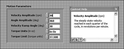
Figure 6-9 shows the Motion Parameters cluster that is used throughout the Torque Hysteresis VI. The controls and labels within the cluster are independently aligned using the Right Edges and Left Edges alignment tools, respectively. The controls are evenly spaced and compressed using the Vertical Compress tool. Each control contains a description, including the Velocity Amplitude, as shown in the Context Help window.

Figure 6-9. Motion Parameters cluster from Torque Hysteresis VI, with the Context Help window displaying the description for Velocity Amplitude. The cluster is neat, compact, and well documented.

This rule cannot be overstated. Clusters form the data infrastructure of most applications and are highly subject to change. Save all clusters as type definitions or strict type definitions, and apply the type definition for each instance of the cluster. This ensures that any changes made to the type definition are automatically applied to every instance within every VI that uses it. This guarantees consistent cluster configurations, substantially streamlining application maintenance. Use the Control Editor window to create or edit the type definition, and use the Type Def. Status ring to specify the control type. Per Rule 6.6, choose the Strict Type Def. if the control has custom properties in addition to the element data types, and choose the Type Def. otherwise. Personally, I prefer strict type definitions over type definitions because I might want to edit the properties of the type definition after I have created multiple instances. Therefore, I can customize the appearance of the cluster or any element, and the properties are applied to all instances. Clone an instance of the type definition by choosing Select a Control from the Controls palette, or drag and drop a type definition from the Project Explorer window. Also, if you need to make a constant that is compatible with the cluster, select Create»Constant from the shortcut menu of one of the terminals of the type definition. Alternatively, select a type definition control file from the Project Explorer window or by using Select a VI from the functions palette, and drag and drop the type definition onto the diagram. Constants formed in this manner maintain compatibility with the type definition.

On the diagram, use the Bundle By Name and Unbundle By Name functions to access and replace the elements of a cluster. These functions provide more flexibility versus Bundle and Unbundle. Specifically, you can access or update any element of the cluster in any order using Bundle By Name and Unbundle By Name. Also, these operations do not break if your cluster changes, unless the specific elements that are being bundled or unbundled are affected. Hence, this rule works together with Rule 6.25 to streamline maintenance. Most important, the name labels uniquely identify the elements of the cluster and provide excellent documentation on the diagram. Because the Bundle and Unbundle By Name functions are sized according to the longest label, keep the control labels succinct and intuitive. Hence, Bundle and Unbundle By Name enhance the maintainability and readability of the diagram.

Note that the strict type-defined clusters of the Torque Hysteresis VI shown in Figure 6-5A are not designed for interactive GUI behavior. Rather, the compression, default fonts, and properties make them less than ideal for GUI VIs such as dialogs. Additionally, there are some considerations with respect to tab key navigation. Individual controls that are not part of a cluster are configured for simple and immediate tab key navigation by default. The tab order of controls on the front panel can be edited by selecting Edit»Set Tabbing Order. The elements within a cluster can also be tabbed according to their cluster order, after the Key Focus property is applied to any element within the cluster. Subsequently, tabbing remains confined to the cluster until Key Focus is applied to a control outside the cluster. Therefore, tab key navigation requires additional programming for a cluster that is not necessary using the controls on the panel.

Figure 6-10 illustrates how a cluster can be used in conjunction with a dialog that prompts the user for the UUT information. The visible area of the panel simply contains string controls that have been customized for GUI interaction, as shown in Figure 6-10A. The UUT Information strict type-defined cluster is actually scrolled off to the side of the panel that is not visible, as shown in Figure 6-10B, along with the error clusters and Cancelled? indicator. Tab key navigation has been disabled for the noninteractive controls. This is accomplished by selecting Advanced»Key Navigation»Tab Behavior »Skip this control when tabbing. Notice that the type-defined cluster is much more compact than the corresponding controls on the panel. Hence, in this example, the controls on the panel are customized for best GUI behavior, and the type-defined cluster is optimized for subVI propagation.

Figure 6-10A. The front panel of UUT Information Dialog contains string controls that are customized for GUI interaction.

Figure 6-10B. The UUT Information type-defined cluster and other controls are scrolled off the visible area of the screen.

The diagram of UUT Information Dialog bundles the data from the interactive GUI controls into the cluster when the OK button is pressed. In Figure 6-10C, we see that the terminals of the Bundle function are ambiguous. The developer has no way of knowing which terminal corresponds to which cluster control without examining the cluster order. Moreover, any changes to the cluster will create maintenance challenges for the developer using this approach. For example, the cluster order might change after adding and deleting or renaming string controls, without changing the number and data type of the elements. This would result in the same configuration as in Figure 6-10C, but an incorrect outcome. Figure 6-10D illustrates proper use of Bundle By Name for bundling the data into the type definition. As we can see, the Bundle By Name function’s terminals are clearly labeled. Also, Bundle By Name is insensitive to the cluster order. If a cluster element is added, removed, or relabeled, the Bundle By Name and Unbundle By Name elements become invalid if they are affected. Therefore, Bundle By Name is much more readable and maintainable than Bundle.

Figure 6-10C. The string controls are bundled into a cluster on the diagram. The terminals of the Bundle function are ambiguous.

Figure 6-10D. Bundle By Name provides terminal labels that improve readability and maintenance.

6.3.2 Special Data Constructs

A few special data constructs include matrix, error, waveform, dynamic, and variant. The former four are variations of arrays and clusters that are predefined by LabVIEW and serve a specific purpose. The real and complex matrices are simply two-dimensional arrays of double-precision floating-point numbers and complex numbers, respectively. These arrays have been customized and saved as type definitions. They are used widely throughout the Linear Algebra VIs in the Math library. Likewise, the error in and error out clusters, used extensively for error propagation, are just clusters.

The waveform data type (WDT) can be considered a special type of cluster consisting of three elements plus attributes. The elements include a start timestamp, t₀; a time interval between data points, dt; and a one-dimensional array of numbers representing the samples of an analog or a digital waveform, Y. The attributes may contain any number of developer-specified name and value pairs. An example is a name or description for the waveform. In addition to the existence of attributes, WDT has conceptually different semantics with respect to math operations than standard clusters. Consequently, the WDT has a palette of dedicated functions for accessing and manipulating its data. Conversely, the standard cluster functions do not support the WDT.

Dynamic is a universal data type used with Express VIs. It was designed for novice developers as a very flexible data type that can store many types of data without learning about data types, data storage, and type conversion. You can wire the dynamic data type to any input terminal or indicator that accepts Boolean, numeric, or waveform data. LabVIEW automatically inserts the appropriate Convert to/from Dynamic Data function when required. In memory, the dynamic data type is represented as an array of analog double-precision floating-point waveforms.

A variant is a self-describing data type that encodes the data name, data type, data, and attributes or information about the data into a generic format. Conceptually, variant can be thought of as a wrapper that converts any data into a new format that is described in a universal manner. In LabVIEW, the variant data type is compatible with the standard used in Microsoft COM and .NET technologies. Specifically, variant is used with DataSocket and ActiveX communication protocol VIs. Additionally, variant is commonly used as a generic data type that passes data defined dynamically during runtime instead of edit time. It allows a data source or server to provide any type of data to a destination or client that can decode and use the data. The functional interface, such as a subVI connector terminal, maintains the variant data type, regardless of the variant’s actual contents. This allows the client and server to be revised without affecting the interface.

The disadvantage of variant is that it is less memory and processor efficient than the conventional fixed data types, and may require additional programming to encode and decode the data within the client and server applications. In LabVIEW, variants are assembled using the To Variant and Set Variant Attribute functions. Alternatively, any LabVIEW data type is automatically converted to variant when wired to an input terminal of type variant. The conversion is denoted by a coercion dot.

6.3.3 Nested Data Structures

As noted previously, arrays and clusters are tremendously flexible data structures. For example, there is no practical limit to the number of dimensions arrays can have, although three or fewer is by far the most common. Also, you can create arrays containing clusters as elements, which can contain arrays and clusters, ad infinitum. Likewise, you can create clusters containing any combination of simple data types, arrays, and clusters, which may contain arrays and clusters. The only limitation is that arrays cannot directly contain other arrays, unless the contained arrays are bundled by a cluster. In any event, there is no practical limit to the number of layers of arrays and clusters within arrays and clusters that LabVIEW allows us to create.

Data constructs containing multiple layers of arrays and clusters are referred to as nested data structures and are considered complicated for two reasons. First, they are confusing for the developer to manipulate on the diagram. For example, changing a single element of data may require multiple calls to Index Array and Unbundle By Name to access the data element, followed by multiple calls to Bundle By Name and Replace Array Subset to rebuild the data structure. These cluster and array manipulation functions are frequently intermixed with nested looping structures used to index through the elements of each array layer. This becomes tedious and confusing after the first two layers.

The second reason nested data structures are complicated relates to how LabVIEW stores them in memory. Clusters are represented by a heading that describes the order and type of the data elements they contain, along with the values of any simple data types, in contiguous memory locations. The data of any arrays, strings, paths, and subclusters are not stored within the cluster. Rather, LabVIEW stores a handle containing the memory location where each multivalued data element is stored. Consequently, nested data structures may be stored as a network of handles and data that is distributed throughout the target computer’s data memory space. The more layers, the more complicated this network can become.

Because LabVIEW manages memory automatically, the complication of a nested data structure’s memory network is transparent to the developer. However, the developer should be concerned with memory efficiency. Specifically, each branch of the nested data structure requires additional memory operations to allocate and manipulate the data. First, most calls to Bundle By Name, Unbundle By Name, and Index Array cause a copy of the data provided at the output of each function to be created in memory. Additionally, as the size of the data contained in any array layer grows, the corresponding memory buffer may have to be reallocated, requiring more memory operations. The previous memory buffers fragment their memory blocks when new buffers are allocated in new locations. Hence, nested data structures use memory less efficiently than simple data structures. Per Theorem 6-1, memory access time is the principal latency in modern computing devices. Frequent operations involving nested data structures can reduce application performance.

Despite these grim-sounding side effects, there are very practical uses for nested data structures that have limits to the number of layers and data size. Nested data structures help organize data in a hierarchical manner. If your target is a modern PC, you probably have plenty of memory resources at your disposal, and you can minimize the impact on performance if the nested data structures are applied properly. Specifically, try to manipulate the nested data at select locations in your application where performance is the least critical.

For example, a nested data structure can be designed to organize a mixture of configuration data, raw acquired data, and post-processed data. The configuration data may be queried from various locations and bundled or unbundled prior to initiating any resource-demanding operations. Accessing the nested data structure should be avoided during the execution of critical tasks, such as high speed data acquisition, deterministic control, and online data processing. Specifically, never bundle or unbundle continuously acquired measurement data into a nested data structure on-the-fly, as it is being acquired. As the size of the data increases, LabVIEW’s memory manager may allocate new memory, causing a latency. Latencies affect the reliability of software-timed tasks, which may result in lost data or unacceptable jitter.

Another method of preventing memory allocation latencies is to predetermine the maximum size of all arrays, including the array layers of a nested data structure, and initialize and maintain them at their maximum length. All array operations subsequent to the initialization can then be performed using the Index Array and Replace Array Subset functions. In this manner, the data structures maintain a constant size, and memory management is limited and predictable.

Use a specific uncommon initial value to help distinguish valid data from initialization data. The NaN constant, which stands for Not a Number, is a particularly useful constant for initializing floating-point numeric arrays. NaN can easily be identified and searched for using LabVIEW’s array functions and cannot be confused with valid measurement data. Additionally, all of LabVIEW’s graph indicators will skip drawing any data points containing NaN.

Figure 6-11 contains an alternative implementation of the Torque Hysteresis VI utilizing a nested data structure to provide enhanced functionality. The controls that comprise the data structure are shown in Figure 6-11A. The UUT Information and Motion Parameters clusters from Figure 6-5A have been combined to form a new cluster, along with an array of cluster that combines the Torque vs Angle and Statistics clusters. The latter array stores data from multiple test runs, reusing the same UUT Information and Motion Parameters for each run. Additionally, the larger cluster is contained within an array, storing data from multiple UUTs that comprise a lot. This data structure contains five layers of nesting, as follows:

1. Torque vs Angle and Statistics subclusters
2. A subcluster containing the latter clusters that stores the data acquired from a single run
3. The Multiple Run Data array, consisting of an array of single run subclusters
4. A cluster that combines the Multiple Run Data together with the UUT Information and Motion Parameters, containing all data for a single UUT
5. The Multiple UUT Data array, consisting of an array of the composite data for the multiple UUTs that comprise a lot

Figure 6-11A. An alternative data structure for the Torque Hysteresis VI has five layers of nesting.

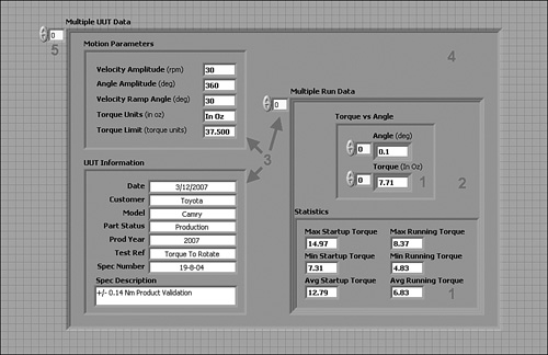
Figure 6-11B presents the enhanced top-level diagram that takes advantage of the nested data structure. There are now two additional looping structures. The inner For Loop allows multiple tests to run on a single UUT, and the corresponding statistics are computed after each run. The middle While Loop allows multiple UUTs to be tested consecutively. Shift registers and wires are used to propagate the nested data structure between each loop. Within the subVIs, the data from each UUT and each test run is appended to the data structure. The application writes the data to file after each UUT but maintains the data in the structure until the end of a lot, at which point a report is generated summarizing the data for the multiple UUTs that comprise the lot. In this example, the nested data structure reduces wire clutter on the top-level diagram by combining multiple structures into one and adds the flexibility to perform multiple test runs per UUT, by storing the data for all test runs performed on multiple UUTs.

Figure 6-11B. The nested data structure propagates among all subVIs of the top-level diagram. The data structure and diagram enhancements facilitate multiple test runs per UUT, multiple UUTs, and organized data with fewer wires.

Figure 6-11C illustrates one possible approach for implementing Run Test VI, in which the Torque vs Angle measurement data is acquired and combined with the nested data structure. However, this approach is not recommended because of the continuous resizing of the arrays using Build Array, and manipulation of the Torque vs Angle subcluster within a time-sensitive acquisition loop. Specifically, the output of each Build Array function has a different array size than the inputs, causing LabVIEW to periodically allocate new memory buffers. Latencies resulting from the reallocation of buffers may cause unacceptable jitter during acquisition. Unbundle and Bundle By Name are used to combine the data with the Torque vs Angle subcluster within each iteration of the While Loop, which is unnecessary additional overhead within the looping structure. Because the While Loop is where the torque and angle measurements are acquired, this is a critical portion of the application, and data manipulation should be minimized.

Figure 6-11C. One implementation of Run Test VI uses the Unbundle by Name, Bundle by Name, and Build Array functions to combine the newly acquired data with the Torque vs Angle subcluster. This implementation is inefficient because the Build Array function continuously resizes the arrays, allowing latencies due to memory allocations during the time-sensitive acquisition task.

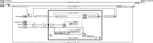
Figure 6-11D contains the diagram of Populate Data Structure VI, a routine that initializes the Multiple Run Data portion of the overall data structure. It generates a Torque vs Angle subcluster, prepopulated with arrays of the NaN constant. Specifically, the maximum number of torque and angle samples that may be acquired per test run is calculated as the product of the Angle Amplitude (deg) and Max Rate (Sa/deg) parameters. An array of NaN is initialized to this maximum length and assigned to both the Torque (In Oz) and Angle(deg) elements of the Torque vs Angle subcluster. Next, the Torque vs Angle subcluster is bundled into the corresponding element of the single run cluster. An array of single run clusters is initialized based on the specified Number of Runs, forming the Multiple Run Data array. The Multiple Run Data array is bundled into the corresponding element of the single UUT cluster. The single UUT cluster then replaces the element of the Multiple UUT Data array corresponding to the UUT Number. Initialization of the nested data structure for multiple test runs using one UUT is complete. Populate Data Structure VI is inserted into the top-level VI just prior to the For Loop, as shown in Figure 6-11E.

Figure 6-11D. Populate Data Structure VI is a subVI that initializes the nested data structure’s Multiple Run Data array with Torque vs Angle data containing the NAN constant.

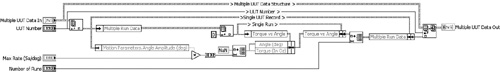
Figure 6-11E. Populate Data Structure VI is inserted into the top-level VI just before the For Loop that performs multiple test runs.

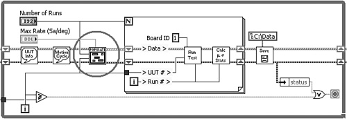
Figure 6-11F illustrates a reliable and efficient method of implementing Run Test VI utilizing the previously populated nested data structure. During the time-sensitive acquisition loop, the data manipulation is reduced to replacing the elements of the torque and angle arrays with real measurements, using the Replace Array Subset function. Because these arrays contain simple data types with constant size, no extra buffers are created and no unpredictable latencies will occur during acquisition. Likewise, Replace Array Subset is used to insert the single run data into the Multiple Run Data array, and the single UUT cluster into the Multiple UUT Data array. The Replace Array Subset function always performs its operation in place, without either moving or making copies of the input data array. This is possible because the data array size is not changed by this function. After the tests are completed, a post-processing routine can simply search for the NaN constant and resize the arrays to their actual length. The post-processing routine should be performed off-line, after any time-sensitive operations have completed, and we are less concerned with performance.

Figure 6-11F. Efficiency and reliability are improved within Run Test VI by replacing the data elements of each layer of the previously populated nested data structure using Replace Array Subset. The data structure remains a fixed size, and extra buffer allocations are avoided.

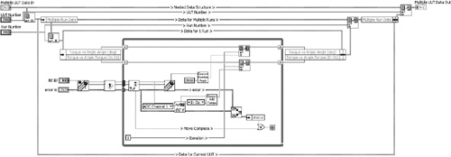
Astute readers may notice coercion dots on the input terminals of the motion control driver VIs in Figures 6-11C and 6-11F. These coercions are caused by dissimilar data types utilized within the driver VIs. Specifically, input and output terminals that are intended to be wired together among the VIs of the driver are comprised of separate type definitions for the controls and indicators. Wiring different type definitions together causes a coercion. Consequently, the driver VIs violate Rule 6.3. However, the coercions are performed on scalar data, which are trivial operations that will not cause latencies.

I would like to add one final note regarding nested data structures. Some references recommend avoiding nested data structures entirely. I disagree with this recommendation. As seen from the previous example, nested data structures can be effectively applied to organize data, increase functionality, reduce wire clutter, and improve maintenance. Performance is controlled by paying attention to where and how the data is manipulated. When applied properly, the organizational and functional benefits of a nested data structure offset the performance considerations. More examples are presented in Section 6.4, “Examples.”

6.4 Examples

This section presents several more examples of proper and improper use of data structures.

6.4.1 Thermometer VI

Thermometer VI, shown in Figure 6-12A, is a subVI that acquires a voltage sample from a thermistor and converts it to engineering units. You may recognize it as a classic LabVIEW training exercise on how to create a subVI. It uses a vertical toggle switch labeled Temp Scale to select between units of degrees Fahrenheit and degrees Celsius. Although there are only two states, a Boolean control is not appropriate because the two states are not logical opposites, per Rule 6.8. Also, the diagram inefficiently computes both units all the time, regardless of the actual unit selected. Figure 6-12B replaces the Boolean with an enum. The enum improves maintenance over the Boolean because more units can be added in the future. Also, the diagram uses a Case structure so that only one unit is computed based on the Temp Scale selection. Additionally, the control and indicator are viewed as terminals, and the Express VIs are viewed as icons. SubVI calls for both versions are illustrated in Figure 6-12C. We see that the Boolean input of Thermometer VI is ambiguous from the caller VI’s diagram. The enum is clearly superior to the Boolean in this example.

Figure 6-12A. Front panel and block diagram for Thermometer VI. The vertical toggle switch for selecting temperature units violates Rule 6.8 because the two states are not logical opposites.

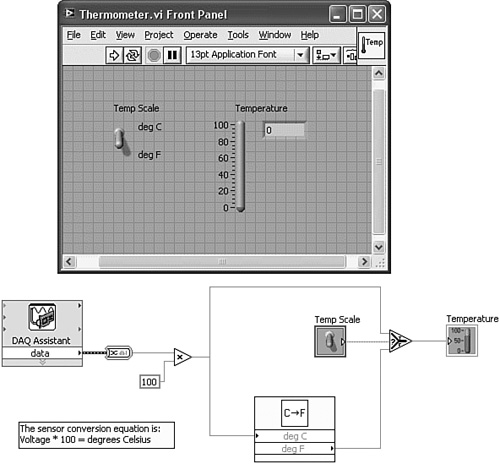
Figure 6-12B. Thermometer with Enum VI uses an enum to select the temperature units. The diagram is more efficient because the conversion to Fahrenheit is not made unless deg F is selected.

Figure 6-12C. The subVI calls for Thermometer VI and Thermometer with Enum VI illustrate that the Boolean is ambiguous from the caller VI’s diagram, whereas the enum is not.

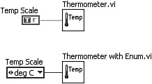
6.4.2 OpenG Variant

The OpenG³ tools include an extensive set of VIs that use the variant data type. Many of these VIs are intended to operate on multiple LabVIEW data types, similar to polymorphic VIs. The LabVIEW data type is converted to a variant, which contains the data type, control name, and data. This information is used to increase the flexibility of the data that can be passed to a subVI through the connector terminals and the operations that can be performed on the data within the subVI. The OpenG tools use this concept to extend the capabilities of the LabVIEW libraries.

When a LabVIEW data type is wired directly to a variant input terminal, a coercion dot appears on the input terminal, and the conversion to variant is performed automatically. However, dissimilar data types are undesirable, per Rule 6.3. Ideally, coercion dots should be avoided for best style. However, the conversion from the LabVIEW data type to variant is unavoidable. As an alternative, the data can be converted to variant using the To Variant function, prior to wiring to the input terminal of the OpenG VI. This method replaces the coercion dot with an explicit function call. While the two methods are functionally equivalent, the explicit conversion conveys that the conversion is deliberate and not an oversight.

For example, in Figure 6-13, the OpenG Empty Array VI is used to determine whether the numeric array wired to its input terminal is empty. The Context Help window indicates a purple wire for the array input terminal, representing the variant data type. The illustration contains three functionally equivalent dataflow paths. The top path connects the array directly to the Empty Array VI, and a coercion dot appears on the VI’s input terminal. The middle path inserts the To Variant function to remove the coercion dot. The bottom path uses the LabVIEW Empty Array? function for the same purpose. The LabVIEW function is polymorphic and does not require a conversion. In terms of performance, the top two paths are identical. The middle path is mildly preferred over the top path because it demonstrates that the type conversion is intended and eliminates the coercion dot. The bottom path is the most efficient overall because the polymorphic function maintains native LabVIEW data types and the type conversion is eliminated.

Figure 6-13. This diagram contains three methods of determining whether the input array is empty. The top dataflow path contains a coercion dot on the input terminal of Empty Array VI. The middle path removes the coercion by explicitly converting to the variant data type. The bottom path uses a polymorphic LabVIEW function to maintain consistent data types.

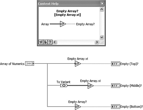
The OpenG Variant Configuration File VIs really showcase the power and flexibility of the variant data type. These VIs read and write data to text files in the standard configuration setting INI file format. They use clusters converted to variants to read or write multiple keys in one subVI call. Figure 6-14 illustrates the use of Write Section Cluster VI. The Motion Parameters cluster is converted to variant and wired to the Section Formatted Cluster input terminal. Write Section Cluster VI uses the data name, data type, and data information that the variant data type provides to create a section of an INI file. The elements of the cluster correspond to the section’s keys, and the name of the cluster is the default section name when the section terminal is unwired. Figure 6-14A shows the source code in which five keys are written using one call to Write Section Cluster VI, and Figure 6-14B shows the resulting section of the INI file. Additionally, the OpenG Write INI Cluster VI populates an entire INI file containing multiple sections. As shown in Figure 6-14C, a nested cluster containing subclusters for each section is wired to the INI Formatted Cluster input terminal. The resulting INI file is shown in Figure 6-14D. In these examples, the variant data type is used to minimize development effort.

Figure 6-14A. The Motion Parameters cluster is converted to variant and written to a section of an INI file using Write Section Cluster VI.

Figure 6-14B. The Motion Parameters section of the INI file resulting from the operation in Figure 6-14A

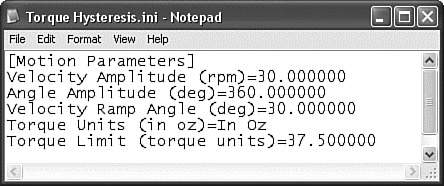
Figure 6-14C. A nested cluster populates multiple sections of an INI file using Write INI Cluster VI.

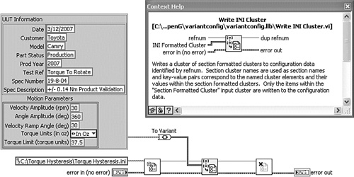
Figure 6-14D. The INI file formed from the operation in Figure 6-14C contains multiple sections.

6.4.3 Haphazard Data

Figure 6-15A contains a data structure that was thrown together rather haphazardly. It consists of an array of clusters containing a subcluster and three subarrays of clusters. It appears unkempt because it violates several of the front panel rules presented in Chapter 3. The alternative presented in Figure 6-15B contains several improvements, including transparent name labels, aligned and compressed controls, and boldface labels with plain-text units in parentheses. Additionally, these data structures contain more controls with fewer layers of nesting. Multiple two-dimensional arrays of clusters in Figure 6-15B are generally more memory efficient than one nested data structure of Figure 6-15A. However, the alternative increases the number of wires and subVI terminals required by a factor of four. The best alternative might be to maintain the single data structure of Figure 6-15A with the organization and neatness of Figure 6-15B.

Figure 6-15A. This data structure is nested and the controls are haphazardly arranged.

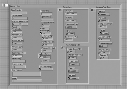
Figure 6-15B. The nested data structure has been divided into four data structures containing fewer layers of nesting, and front panel style rules have been applied to dramatically improve the appearance of each control.

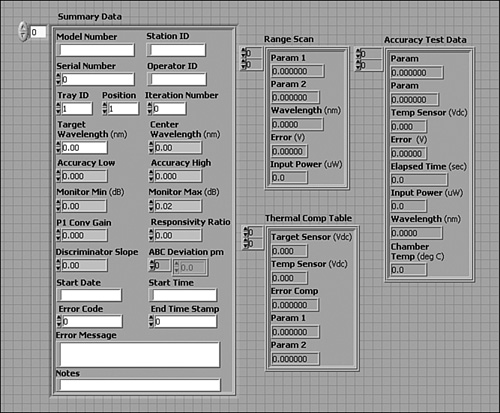
6.4.4 Centrifuge DAQ VI

Centrifuge DAQ System VI, also discussed in Sections 3.5.4 and 4.4.6, is an application that performs dynamic measurements from soil samples in the payload of a centrifuge. The front panel shown in Figure 6-16A is highly configurable, allowing the user to configure a wide variety of signal conditioning modules. The hardware supports up to six SCXI chassis containing any combination of relay, accelerometer, LVDT, strain gage, voltage, and thermocouple conditioning modules. Any number of these modules can reside in any slots of any chassis. Each module type has a different set of programmable parameters, such as excitation voltage, signal amplification gain, filtering, bridge completion, scaling factor, and engineering units. These parameters are configured using a set of nested data structures. When the user selects a sensor type using the Sensor Selection listbox control on the left, one of seven data structures becomes visible. Each data structure is an array of cluster containing one element per SCXI module. This allows each module to be configured independently. Figure 6-16B shows the data structure used to configure strain gages. Its appearance is controlled programmatically using Property Nodes. Also, on the front panel, the array index control is normally not visible and the control’s background color is transparent.

Figure 6-16A. The GUI VI panel for a highly configurable centrifuge data acquisition system

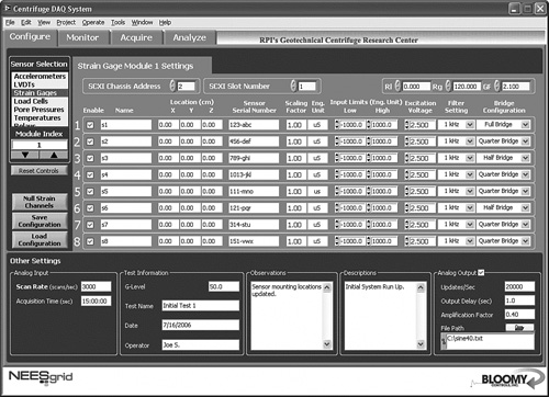
Figure 6-16B. This array of cluster containing strain gage configuration parameters is one of seven data structures used on the Configure tab to configure a corresponding SCXI module type. On the GUI VI panel, the array index control is not visible and the background is transparent.

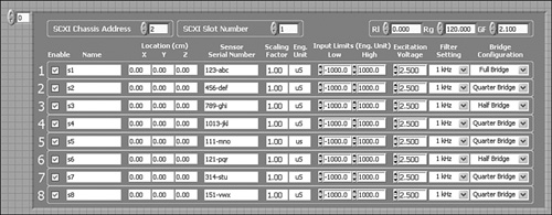
Figure 6-16C contains a code snippet of the application’s configuration state. Multiple nested data structures containing the configuration data for each module type are bundled into another more complicated data structure. This larger structure’s sole purpose is to reduce the number of terminals and associated wire clutter for the subVI that follows. The nesting of this data structure might be a concern if the data was accessed during a time-sensitive routine. However, this data structure contains only configuration data, which is accessed and programmed only before the critical data acquisition routines begin. Therefore, the complexity of this data structure does not affect the performance of the critical task.

Figure 6-16C. The configuration routine bundles data structures to form a complex data structure that is passed into the subVI. Each data structure is an array of cluster containing configuration parameters for a module type, similar to Figure 6-16B.

Endnotes

¹ The LabVIEW online help topic “VI Memory Usage” contains useful information concerning memory usage.

² NI Instrument Driver Guidelines, Control/Indicator Naming and Data Representation.

³ OpenG is an organized community committed to the development and use of open source LabVIEW tools. The URL is www.openg.org.