Money and Wealth in an Open Economy Income–Expenditure Model1
CARLOS A. RODRIGUEZ
The purpose of this chapter is to analyse some of the dynamic implications of the endogeneity of the money supply implicit in a trading world with fixed exchange rates.2 The world we choose to represent is a Keynesian one where prices are constant and outputs are responsive to changes in aggregate demands. Models where prices are fully flexible and outputs are constant or growing at an exogenous rate can be found in Prais (1961), Mundell (1968), and Johnson (1972). Despite the wide difference in assumptions, both types of models bear the common characteristic that the balance of payments is one of the channels through which countries can adjust their actual to their desired holdings of real cash balances.
The principal features of the model used are:
(a) A liquidity preference function which expresses the desired ratio of holdings of real cash balances to other financial assets as a function of the interest rate. Any given size of the portfolio is assumed to be always held in the desired ratio (composition equilibrium); the size of the portfolio itself, however, need not be always equal to the long-run desired value.
(b) An expenditure function which depends on both the level of income and the magnitude of the discrepancy between the actual and the desired holdings of financial assets.
(c) The possibility that domestic income and—when capital is immobile—the interest rate adjust in response to domestic monetary disturbances.
Our main results could be summarised as follows: domestic monetary policy affects income and the interest rate in the short run. In the long run, the endogeneity of the domestic money supply implies that domestic monetary policy will have a permanent effect on other domestic variables—in addition to international reserves—only if it contributes to changes in the world’s supply of money. Thus, in the case of a small country—whose repercusions on the rest of the world are ignored—an expansion in the domestic money supply will not be feasible in the long run and any attempt to do it by printing new money will be matched by an equivalent reduction in the stock of international reserves with no effective change in the domestic money supply.
Section 1 develops the basic structure of the model. Section 2 applies it to a small country. The concept of the ‘small country’ used in this chapter is not defined in the traditional sense as a country facing a perfectly elastic foreign demand for its exports since usually it is incompatible with the existence of a fixed supply price of exportables (in terms of domestic currency) and a fixed exchange rate. Rather, the country is ‘small’ in that changes in its level of imports or reserves have a negligible effect on the rest of the world’s aggregate expenditures and thus on the demand for the country’s exports. Under those circumstances, given the exchange rate and the fixed domestic supply price of exportables, the quantity demanded of exports is a constant, X0. Section 3 abandons the small-country assumption and studies the monetary interactions of a two-country world economy. Throughout the chapter it is assumed that securities are not traded internationally.3
1 THE DESCRIPTION OF THE ECONOMY
It is assumed that output in each country is in perfectly elastic supply at a given price level. To abstract from the effects of economic growth it is assumed that the demand for net investment is zero at all times.
A. Aggregate Expenditures
Whenever the existing stock of financial assets is equal to the desired long-run stock, it is assumed that individuals will want to spend all of their current income. We will therefore define the following expenditure function:
![]()
where
| Z: | Aggregate domestic expenditures, |
| Y: | Current domestic income, |
| A: | Actual stock of financial assets, |
| Ad: | Desired stock of financial assets, |
| a: | Desired speed of adjustment of an excess stock demand for assets. |
Of total expenditures, a constant fraction, m, is spent on foreign goods and the rest on domestic goods.4
B. Financial Assets and Liquidity Preference
The stock of financial assets is the sum of three elements:
(i) The stock of money, H.
(ii) The value of common stock owned by the private sector: peE0 = cY/r where E0 is the number of pieces of common stock (it is fixed due to the absence of net investment); с is the fraction of profits in income (assumed constant); pe is the price of each piece of common stock and r is the interest rate.
(iii) The value of government debt held by the private sector: pB B, where pB is the price of each government bond and B is the quantity of such bonds.
Government debt is assumed to be a perfect substitute for common stock, so the interest rates on both types of assets are the same. Each government bond pays $1 per year so pB = 1/r and B represents the annual stream of payments on government debt. It is assumed that the service of the public debt is financed from income taxes so that a change in B does not affect personal income. It has been argued that if individuals capitalise the future stream of taxes necessary to pay interest on that debt then government debt should not be included in the calculation of the wealth of the private sector—see Mundell (1971).
We will assume that the market does not capitalise future taxes on income streams and thus we consider the full amount B/r as wealth. Notice that even if B/r were not considered as wealth, it would anyway affect other variables of the economy through liquidity preference. The total stock of financial wealth of the private sector is therefore:
![]()
Individuals are assumed to decide on the composition of their portfolio only on the basis of the returns on the available assets. We thus postulate a liquidity preference function similar to the one used in Metzler (1951), where the desired ratio of money holdings to other financial assets is a declining function of the interest rate,
![]()
It is further assumed that the interest rate adjusts such that the liquidity preference is always satisfied. From equations (2) and (3) it follows that the value of financial assets at any moment will depend on the value of money holdings, the number of outstanding government obligations and the level of income,
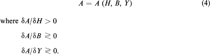
An increase in H always raises A since, in addition to its own impact—in (2)—it also depresses the interest rate—by (3)—and thus raises the value of other financial assets outstanding. This however does not hold for increases in the supply of other financial assets since the change in their total value will depend on the elasticity of demand; this accounts for the indeterminacy of the sign of δA/δB and δA/δY.
The desired stock of financial assets is taken to be a constant fraction, k of income,
![]()
From (1), (4) and (5) we get the expression for aggregate expenditures,
![]()
Finally, it is assumed that the short-run marginal propensity to spend out of an increase in income is positive, but less than unity:
0 < δZ/δY = 1 + a(δA/δY – k) < 1.
This in turn implies that
– 1 < a(δA/δY–k) < 0.
At any moment B and H are given and thus short-run equilibrium is obtained at that level of income which is demanded. The demand for domestic output, in turn, is the sum of the demands by domestic consumers—total expenditures minus imports—and by foreigners—X0. Thus short-run equilibrium is attained when (1 – m)Z + X0 = Y or, rearranging terms, when:
![]()
which implies that any excess of domestic expenditure over income must be validated by a trade deficit.
In the absence of capital mobility or private holdings of foreign exchange, the fixed exchange rate system requires that any trade deficit (surplus) be financed by an equivalent loss (gain) in international reserve holdings of the monetary authority. If those changes in international reserves are not sterilised by the monetary authority, the domestic money supply must change by the same magnitude as the stock of reserves—assuming for simplicity that the exchange rate and the high power money multiplier are unity. It follows that the path of the domestic money supply, in the absence of other sources of money creation, is given by:
![]()
From equations (6) and (7), the condition for internal balance can be written as:
![]()
this condition determines the level of income for any given H, B and X0. This level of income, in turn, determines—from (8)—the rate at which H will be changing. The model is described graphically in Figure 9.1 where the domestic money supply (H) is depicted along the horizontal axis and domestic income (Y) along the vertical axis. The curve Y = Y(H) represents the combinations of Y and H—given B and X0—that are consistent with internal balance and it corresponds to the locus of short-run equilibria. This schedule is upward sloping since a larger H increases aggregate demand by raising the value of assets; to restore equilibrium, output must be raised.5
The Ḣ = 0 locus represents the combinations of Y and H—given B—that are consistent with a zero trade balance and thus the supply of money remains unchanged. This schedule is downward sloping since an increase in H raises expenditures and imports, generating a trade deficit. A reduction in expenditures through a lower income restores trade balance.6
The long-run values Y* and H* are obtained at the unique intersection of the Y(H) and Ḣ = 0 schedules. It should be noted that at this intersection X0 = mY*. This can be easily verified by inspection of equations (7), (8) and (9). Thus the long-run level of income (Y*) is solely determined by the amount of exports and the propensity to import.
Consider the effect of raising the quantity of money from H* to H1, in Figure 9.1. Initially, income must rise to Y1 according to the relation Y = Y(H). Since at this higher income and money supply there is a trade deficit—any point to the right of the Ḣ = 0 schedule implies a trade deficit—the domestic money supply starts to decrease. This process continues as long as Y > Y*. Thus an increase in H above H* will raise income only for a transitional period. Eventually all of the original rise in H will be offset by a cumulative loss in international reserves through the balance-of-payments deficits. On the other hand, a policy of government expenditures financed by printing money will succeed in raising income in the long run but at the cost of a continuous loss in reserves that is equal to the amount of government expenditures. In this case the internal balance condition becomes:

Figure 9.1.
a(l – m) [A(H, Y, B) – kY] = mY – X0 – G,
where G is the level of government expenditures. The money supply will change according to:
Ḣ = G + X0 – mY – am [A(H, Y, B) – kY];
thus when eventually Ḣ = 0, the country will be losing reserves at the rate G = mY – X0 although income has now been raised to the higher level (X0 + G)/m. Clearly this higher level of income can be sustained only as long as the country has enough reserves to cope with the continuous implied trade deficit.
A once and for all increase in the amount of government debt outstanding will not affect the long-run level of income, although it will affect the long-run holdings of money and the interest rate. It will, however, affect income in the short run and this effect depends on the sign of δA/δB which in turn determines whether the schedule Y = Y(H) shifts up or down due to a change in B.7
If δA/δB is positive, an increase in B will raise the interest rate but the over-all value of financial assets will be higher so that expenditures, and thus income, will also rise. This initial rise in income will, however, be transitory since at this higher level there is a trade deficit and H will be falling until income is back at the equilibrium level Y* = X0/m. At this point the interest rate must be higher than its value prior to the increase in government debt since now, at the same income, there is less money and more bonds. We conclude that in the case of a small country, monetary policy or the stock of government debt outstanding can affect the level of income only in the short run—unless a continuous loss in reserves is allowed for.
We now generalise the model of the last sections by considering the interaction between the home country and the rest of the world. If the home country does not have a negligible size, changes in its imports or in its holdings of international reserves will affect other countries’ incomes and money stocks. Given fixed exchange rates, changes in the money supply of any one country, in the absence of capital movements, can be due either to a non-zero trade balance or to a pure monetary creation by the monetary authorities. Since a trade surplus for one country must be a trade deficit for the rest of the world, it follows that, in so far as no government resorts to pure monetary creation, the world money supply will remain constant over time. To the extent that some government(s) do resort to a pure monetary creation, their actions will increase the world supply of money and therefore will have a permanent effect on the income levels of all countries. These effects will, however, be independent of the country in which the changes in the money supply originated.
For simplicity, consider the rest of the world as a single country and assume that demands for imports depend on income rather than on expenditures. The magnitudes for the rest of the world are referred to by an asterisk (*). Since exports of the home country must be imports of the rest of the world—and vice versa—the internal balance conditions for the home country and the rest of the world are, respectively:
![]()
In the absence of a pure monetary creation, an increase in the domestic money supply must be matched by an equal decrease in the foreigner’s money supply, which in turn must be equal to the trade surplus at home and the trade deficit abroad. We can thus postulate:
![]()
with the implication that, at any moment,
![]()
where ![]() is the world’s supply of money and is constant.
is the world’s supply of money and is constant.
It then follows from (10) – (13) that long-run equilibrium is defined by:

These conditions imply that for long-run equilibrium, all countries must be satisfied with their asset holdings—by (14a) and (14b)—and, in addition—by (14c)—those assets are not changing over time. From (14a) – (14b) we obtain a relation between Y and Y* indicating the levels of income for which both countries satisfy their demand for assets—given the world’s money supply and the stocks of government bonds. This relationship (in Figure 9.2) is downward sloping since an increase in domestic income requires an increase in the domestic money supply and thus a reduction in the foreigner’s money supply, which in turn implies a reduction in income abroad.8

Figure 9.2.
Equation (14c) describes the pairs of Y and Y* for which the distribution of the money supply between countries is unchanged. As can be seen, this relation depends only on the propensities to import in each country and is independent of the world’s supply of money.
The world long-run equilibrium for a given set (![]() , B, B*) is shown in Figure 9.2. The upward sloping schedule, Y = Y*m*/m describes the locus for which Ḣ = 0. The downward sloping schedule Y = Y(Y*,
, B, B*) is shown in Figure 9.2. The upward sloping schedule, Y = Y*m*/m describes the locus for which Ḣ = 0. The downward sloping schedule Y = Y(Y*, ![]() , B, B*) represents the locus of Y and Y* for which both countries are on their desired demands for assets. Long-run equilibrium is, of course, attained at the intersection of both schedules.
, B, B*) represents the locus of Y and Y* for which both countries are on their desired demands for assets. Long-run equilibrium is, of course, attained at the intersection of both schedules.
The stability of the long-run solution is guaranteed by our assumption that the short-run marginal propensities to spend are positive but less than unity.9
The effect of an increase in the world money supply is to shift the Y(Y*, B, B*, ![]() ) schedule upwards and thus to raise income in both countries. The proportion in which the increase in world’s income is distributed among countries depends only on the propensities to import in each country. Since the long-run equilibrium conditions depend only on the total world money supply and not on its initial distribution among countries, it follows that the long-run effects of a change in the world supply of money are independent of the country which originated the change. As in the case of a small country, the effects of changes in the stocks of outstanding government debts depend on the signs of δA/δB and δA*/δB*.
) schedule upwards and thus to raise income in both countries. The proportion in which the increase in world’s income is distributed among countries depends only on the propensities to import in each country. Since the long-run equilibrium conditions depend only on the total world money supply and not on its initial distribution among countries, it follows that the long-run effects of a change in the world supply of money are independent of the country which originated the change. As in the case of a small country, the effects of changes in the stocks of outstanding government debts depend on the signs of δA/δB and δA*/δB*.
Having shown the nature and the stability of the long-run solution, we now turn to the dynamics of adjustment. From equation (10) we obtain a relation Y = f(Y*, H, B) describing the combinations of domestic and foreign income that are consistent with internal balance at home, given the domestic money supply. The slope of this schedule is
![]()
Similarly, from (11) we obtain:
Y = g(Y*, B*, H*),
which shows the pairs of incomes consistent with internal balance abroad, given the foreign money supply. The slope of this schedule is:
![]()
It is easy to verify that increases in H will shift the f(.) schedule upwards and increases in H* will shift the g(.) schedule downwards.10 Given any initial distribution of the world supply of money between countries, short run equilibrium is obtained when:
f(Y*, B, H) = g(Y*, B*, H*) = Y
Figure 9.3 shows such a short-run equilibrium position at point Q. Since, as depicted, short-run equilibrium is in the region where m*Y* > mY, H must be rising over time and H* decreasing. Thus, as time passes, both schedules must shift upwards until long-run equilibrium is obtained when their intersection is on the Ḣ = 0 line—when mY = m*Y*. Starting from a long-run equilibrium
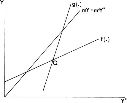
Figure 9.3.
position, Figure 9.4 shows the effects of a once and for all increase in the money supply in the home country. Starting at point A, an increase in H will shift the f(.) schedule upwards from f0 to f1 and thus will generate a short-run equilibrium at point B where both incomes are higher than before. At B, however, the home country will be running a trade deficit and thus Ḣ < 0, Ḣ* > 0, and both the f(.) and the g(.) schedules will start shifting to the right. Over time, it is clear that what happens with both incomes depends crucially on the speed at which both schedules are shifting. In particular, it is interesting to note the role of the speeds of adjustment to stock disequilibrium (a and a*) in the determination of the behaviour of both incomes over time. After the new short-run equilibrium at B, a redistribution of money from the home country to the rest of the world will take place until a new long-run equilibrium position is attained. Thus the path of Y and Y* will depend on how this redistribution of money affects aggregate demands in both countries. There are three main possible outcomes indicated as paths 1, 2, and 3 in Figure 9.4:
(a) Path 1: Both Y and Y* continue to rise after B has been attained. This case is more likely the larger is a* and the smaller is a. This is so because as H decreases, a small a implies a small reduction in aggregate expenditures at home and conversely, a large a*
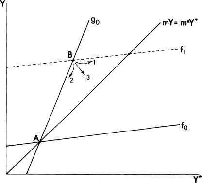
Figure 9.4.
induces a large increase in aggregate expenditures abroad, since H* is rising. In this case, it is more likely that the increased foreign demand for domestic products will outweigh the reduced demand by domestic residents with the net effect that both incomes tend to rise.
(b) Path 2: Both Y and Y* start to decrease. This case is more likely the larger is a and the smaller is a*. This is so because a reduction in H induces a large decline in domestic expenditures while the rise in H* does not induce a large increase in foreign expenditures.
(c) Path 3: Y decreases and Y* increases: This is an intermediate case between (a) and (b) and its likelihood will depend on the precise relationship between all of the variables involved.
CONCLUSIONS
In this chapter we have analysed the implications of a system of fixed exchange rates on the short- and long-run effects of monetary policy. The main conclusion is that, independently of the size of the country, the domestic money supply cannot be controlled, in the long run, by the monetary authorities unless a continuous loss in international reserves is allowed for. Despite the fact that the world described is a Keynesian one where income and the interest rate adjust in response to domestic monetary disturbances, the long-run effects of monetary policy are similar to the ones obtained in models where the real sector is assumed independent of the monetary sector. We have described, both for a small country and for a two-country world, the short-run (impact) effect of changes in the domestic money supplies and the long-run effects together with a description of the dynamic adjustment process, in which the speeds of adjustment to assets disequilibrium were shown to play a crucial role.
REFERENCES
Frenkel, Jacob, ‘A Theory of Money, Trade and the Balance of Payments in a Model of Accumulation’, Journal of International Economics, I (2) (May 1971), 159–87.
Johnson, Harry G., ‘The Monetary Approach to Balance of Payments Theory’, Journal of Financial and Quantitative Analysis, vii (March 1972), 1555–72.
Metzler, Lloyd A., ‘Wealth, Saving and the Rate of Interest’, Journal of Political Economy, 59 (1951), 93–116.
Mundell, Robert A., International Economics (Macmillan, 1968).
Mundell, Robert A., Monetary Theory (Goodyear, 1971).
Prais, S. J., ‘Some Mathematical Notes on the Quantity Theory of Money in an Open Economy’, IMF Staff Papers, 8, no. 2 (1961).
Swoboda, A., and Dornbusch, R., ‘International Adjustment, Macroeconomic Policy and Monetary Equilibrium in a Two-Country Model of Income Determination’, in International Trade and Money, edited by A. Swoboda and M. B. Connolly (London, George Allen & Unwin, 1973), 225–65.
1 I want to thank Rudiger Dornbusch and Jacob Frenkel for their comments and suggestions on a previous version of this paper.
2 Swoboda and Dornbusch (1973) analyse essentially the same problem. This model differs from theirs in that it includes a more detailed specification of the role of assets and liquidity preference in the determination of aggregate expenditures.
3 Trade in securities will not affect the main long-run predictions of the model. If it were to be considered, national income and not domestic income would have to be the relevant variable in the determination of expenditure decisions; on this see Frenkel (1971).
4 In the two-country case analysed in section 2 it is assumed that imports depend on income rather than on expenditures. This assumption simplifies considerably the presentation and does not affect any of the long-run results. The short-run dynamics, however, could be different from the one obtained in that section if imports were to depend on expenditures.
5 The slope of this schedule is:
![]()
6 The slope of this schedule is:
![]()
7 Whatever the direction of the shift in the Y = Y(H) schedule, the Ḣ = 0 schedule will shift horizontally by the same magnitude such that their intersection will remain at the same level of income Y* = X0/m. The horizontal shift in both schedules due to changes in B is δH/δB = –(δA/δB)/(δA/δH).
8 The slope of this curve is:
![]()
The schedule shifts with changes in the world money supply according to:
![]()
9 From differentiation of (10), (11), and (13) and using (12) we obtain:
![]()
since
![]()
10 These shifts are given by:
![]()