13

Aspects of the Monetary Approach to Balance-of-Payments Theory

An Empirical Study of Sweden¹

A. HANS GENBERG

INTRODUCTION

In this chapter we shall attempt to provide an empirical analysis of some aspects of the monetary approach to balance-of-payments theory. We shall concentrate on a few but in our view crucial hypotheses regarding the nature of a small economy and its relationship with the world at large.

Firstly we take up the question of goods and asset market integration in the world. This is one of the building blocks of the monetary approach which stresses the importance of world rather than individual country equilibrium in the determination of prices and interest rates. Secondly we discuss the link between reserve flows and the domestic money stock and show that this is the avenue through which monetary equilibrium is reached in an open economy. After identifying and estimating empirical demand functions for money in Sweden, some conclusions with respect to the effect of monetary policy are discussed. The final section combines the obtained evidence in a monetary interpretation of reserve flows. Some questions regarding the possibility of lagged balance-of-payments adjustment and central bank sterilisation are also taken up.

MARKET INTEGRATION IN THE WORLD ECONOMY

Market integration and interdependence among national economies can be studied from several angles. In theoretical work it is common to link structural models of individual economies and to simulate the effects of policies allowing for interaction between countries.² In practice, when the true structures of the models are not known, this approach might lead to effectively specifying a certain type of interdependence rather than letting the data decide the issue. Hence we shall concentrate on a more pragmatic approach by directly comparing price series in goods and asset markets of several countries to determine how closely they move together. For each market we shall first consider intercountry comparisons and then look somewhat more closely at the Swedish data.

Goods Market

Comparison of consumer price indices between countries implicitly involves comparing prices of both internationally traded and non-traded goods. Thus, while we expect traded goods prices to be kept in line through arbitrage, there will be some room for variance in domestic goods prices. The degree of correspondence between countries will depend on the elasticity of substitution in consumption and/or production relative to the traded goods both at home and abroad.

Apart from the existence of non-traded goods, price indices might change at different rates due to non-conformity in weighing patterns, collection practices, timing, coverage, treatment of indirect taxes, etc. If, for instance, the price of heating oil carries a large weight in a Swedish consumer price index relative to an Italian one, an equal change in the price of oil in both countries will make for unequal change in the price indices. While this is a feature we wish a price index to have, it can not be used as evidence against the market integration hypothesis.

Assuming that the artificial differences introduced in constructing the indices can be approximated by a random disturbance term, we can test the market integration hypothesis as follows.

Let (Ṗ/P)_i,t be the inflation rate in country i at time t. Then we can write

where is the world rate of inflation and a_i,t represents the systematic difference between country i’s and the world’s rate of inflation at time t due to the specific economic environment in country i. u_i,t is a disturbance term. Under the hypothesis that all countries have the same rate of inflation, we see that

a_i,t = 0 for all i and t.

A simple analysis of variance procedure was used to examine this hypothesis for the period 1959–II to 1970–II. Quarterly rates of change in the consumer price index (as reported by the OECD)³ were computed for the following countries: Austria, Belgium, Denmark, Finland, France, Germany, Ireland, Italy, Japan, the Netherlands, Norway, Portugal, Sweden, Switzerland, United Kingdom, and U.S.A. Since some countries did alter their exchange rate during the sample period, we deleted the observations which were affected under the assumption that adjustment to the exchange rate change was complete within the quarter.⁴ The sample period was also split into three groups according to the average rate of inflation of the whole set of countries. The relevant F-ratios for the analysis of variance procedure are presented in Table 13.1.

Table 13.1 F-Statistics to Test Equality of Inflation Rates Between Various Countries

Period	Average rate of price change (% per year)	F-ratio	Critical F-values
			25% point:
Period 1a	0–2%	F15,47 = 0.55	F15,60= 1.38
			25% point:
Period 2b	2–4%	F15,254 = 2.63	F15, ∞ = 2.40
			25% point:
Period 3c	4–6%	F15,183 = 1.12	F15, ∞ = 1.40

^aThe 1962–III observation for the Netherlands was deleted from the sample due to the unusual behaviour of food prices. (Whereas the CPI including food fell from 101 to 97 between the 2nd and 3rd quarters, the index excluding food stayed constant at 97.)

^bThe 1962–I observation for Sweden and 1962-1V observation for Denmark were excluded since large changes in indirect taxes were made during these quarters.

^cThree observations for Austria and the Netherlands, two for Ireland and one for Sweden were deleted so that breaks in the series (Austria and Ireland), indirect tax changes (the Netherlands and Sweden), and extraordinary food price changes (Austria, Ireland, and the Netherlands) would not distort the results.

The analysis of variance technique calls for computing the ratio of the sum of squared differences of country means from the over-all mean to the sum of squared differences of within country observations from the country means.⁵ Thus a high value of the F-ratio would indicate significant differences between the country mean rates of inflation. Under the null-hypothesis the ratio will have the F-distribution, given certain assumptions about the error term (normality and independence). Thus we can attach significance levels to the rejection or acceptance of the null-hypothesis. The critical F-values are given in the last column of Table 13.1.

By comparing the last two columns of Table 13.1 for the first and third periods we can reject the hypothesis that inflation rates differ significantly between countries. But for the second period we must conclude that a difference does exist. This appears to be due mainly to two factors. Firstly the average rate of inflation in Japan seems to be significantly larger than in the other countries during this period. Secondly, it might be that the many devaluations in 1967 had dissimilar price index movements associated with them lasting longer than a quarter as assumed above. The F-ratios of period 2 which includes observations immediately before and after those devaluations would accordingly be affected. These speculations are supported by the fact that when calculations were made for only the countries⁶ which maintained fixed exchange rates vis-à-vis the U.S.A. during the whole sample period, the F-ratios⁷ were 1.98 with Japan included and 1.07 with Japan excluded.

Since the assumptions needed to apply the F-test might not be met in our sample, a different kind of comparison was also carried out. Rates of change in the quarterly consumer price index for fifteen U.S. cities⁸ were computed and the same ratios (see Table 13.2) were formed as in the country analysis.

It is evident from Tables 13.1 and 13.2 that the differences between OECD countries are no greater on the average than those between cities within the United States. Thus, if we believe that the whole of the U.S. can be treated as a single market in a macroeconomic context, then the area composed of the above countries can be treated likewise.

Table 13.2 F-Statistic to Test Equality of Inflation Rates Between U.S. Cities

Period	F-ratio
Period 1	F14,375= 0.79
Period 2	F14,222 = 0.75
Period 3	F14,195 = 1.59

For a country like Sweden the unified market hypothesis implies that the rate of inflation will be exogeneously determined under a fixed exchange rate system, because Sweden is too small to have a noticeable impact on world prices. To check whether this implication is supported by the data, we postulate that the Swedish rate of inflation is equal to a constant times the world rate of inflation⁹ plus a stochastic error term as in

We expect to find a value of с close to unity if our hypothesis is true. A regression using quarterly rates of change in the Swedish consumer price index as the dependent variable did give an estimate significantly different from unity at the 5 per cent level (see Table 13.3, row 1). This is likely due to bias towards zero in the estimate as a consequence of measurement errors in the independent variable. In this case we can compute bounds for the estimate of с by reversing the role of the dependent and independent variables (see Table 13.3, row 2). This procedure yielded point estimates of the bounds of 0.78 and 0.96 respectively. Although these are still somewhat low, a two-standard-error confidence region of the bounds will include unity.

Table 13.3 Relationship Between the Rates of Inflation in Sweden and the Rest of the World

Dependent variable	Independent variable	Coefficient (standard error)	с	R2
Sweden	World	0.78 (0.07)	0.78	0.41
World	Sweden	1.04 (0.10)	0.96	0.10

Together with the previous evidence these results support the view that Sweden is a small part of an integrated world goods market.

Asset Markets

Asset markets in different countries have often been looked upon as separate entities with only limited interdependence due to various controls and restrictions on international movements of capital. It has been argued that considerable profits could be made from equity portfolio diversification¹⁰ if these restrictions were lifted, and that capital flows between countries respond to observed interest rate differentials (or changes in these).¹¹

Another view of the international asset markets is that, controls notwithstanding, they approximate a highly integrated market where diversification opportunities are already exploited, and where observed yield differentials are due to exchange-rate-risk, political-risk, and other types of risk, and correspond to equilibrium values.

In the following we shall present evidence consistent with integrated market hypothesis which can be weighed against the evidence for the alternative view.

Equity Market

In two articles¹² Agmon investigated the equity markets in Germany, Japan, U.K., and U.S.A. and concluded after tests carried out on both market indices and individual share prices that his data were consistent with the single-market hypothesis. Furthermore, from the point of view of the U.S. investor, the removal of obstacles to capital flows would not necessarily imply expanded profit opportunities.¹³

Agmon also found that the New York Stock Exchange seemed to determine the prices on the other markets in the sense that the correlation between stock price changes in Frankfurt, London, and Tokyo was small after removal of the common New York effect. Treating prices on the New York Stock Exchange as world market prices we shall here carry out a test of the single-market hypothesis applied to Swedish stock prices. Table 13.4 contains results from regressions of the form

Table 13.4 Stock Price Regressions for Sweden and Germany

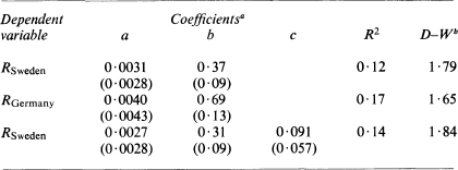
^a Standard errors are given in parentheses.

^b Durbin–Watson statistic.

where R_t is the monthly rate of change in the relevant stock price index, i.e.

R_t = log(P_t/P_{t – 1}),

P_t = index of stock prices at time t.¹⁴

Comparing our results with those obtained by Agmon we note that the coefficients as well as the R² are of the same order of magnitude. We see also that the German index does not contribute much to the variations in Swedish stock prices after allowing for the U.S. effect, supporting the view of the New York Stock Exchange as the centre of a world equity market.

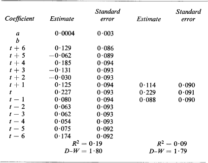
We can also check whether leads or lags in the U.S. index play a significant role in the explanation of the Swedish index. In a unified and well functioning market all but the current value of the independent variable should have a negligible effect. Table 13.5 presents estimates from the regression

The coefficient estimates and their standard errors clearly support the unified market hypothesis.

Table 13.5 Lead-Lag Analysis of Swedish Stock Price Changes

Bond Market

The question of financial market integration as measured by the similarity of interest-rate movements in various countries has recently been studied by several economists. In the course of examining the policy implications of the Euro-dollar market, Scott¹⁵ presented some evidence indicating that short-term interest-rate differentials have tended to decrease since the moves towards currency convertibility in 1958. This is consistent with the view that the development of the Euro-dollar market has increased integration by acting as a link between individual nation’s financial markets. Cooper¹⁶ and Argy and Hodjera¹⁷ similarly showed that the variance of national market interest rates at each point in time tended to decrease from 1958 until the middle of the sixties, after which it levelled off or increased slightly. This can be interpreted as a sign of initially increased interdependence subsequent to convertibility halted by the attempts on the part of governments to reverse the trend by imposing restrictions and controls on international capital movements. The increased interest rate divergence after the middle sixties might also be a reflection of the increasingly troubled foreign exchange markets, culminating in the currency crises towards the end of the decade. Since yield differentials between securities of different currency denomination reflect foreign-exchange-risk and other types of risk, it is not surprising to find larger differentials in periods when exchange-rate changes are contemplated.

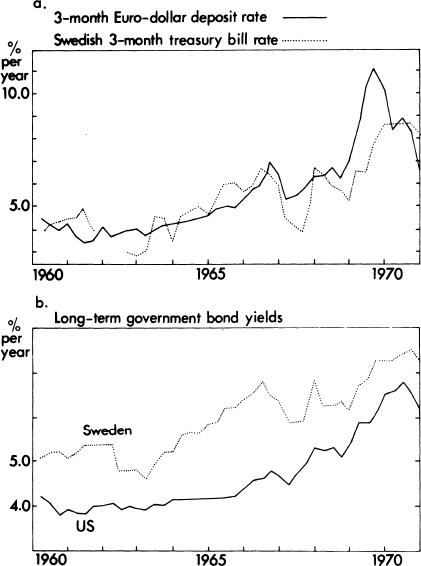
Figure 13.1. Interest-rate comparisons.

Although controls and restrictions tend to decrease financial integration it is clear that the profit opportunities associated with avoiding them imply behaviour working in the opposite direction. A good example is the recent Swedish experience.

In attempts to assure cheap credit to the government and for housing construction, the central bank has placed various controls on the domestic bond market. Besides requiring banks and other financial institutions to hold certain portions of their portfolios in the form of government and mortgage bonds, the central bank controls open public borrowing by firms by requiring its approval for all bond issues. To give the system a chance to work, extremely strict controls have also been placed on international movements of financial capital.

As a result of the official rationing programme, however, a large trade credit market has developed in Sweden. Although data are not officially available, it is believed that the interest rates prevailing in this market are very closely related to Euro-dollar deposit rates due to intermediation performed by exporters and importers receiving or extending international trade credits. They can do so in the context of unregulated current transactions simply by varying the leads and lags in payments for shipments.

The existence of this source of foreign borrowing and lending implies that the marginal cost of credit to a Swedish firm will be closely related to the rate of interest prevailing abroad, and also that the government-controlled interest rates must be kept in line to avoid large and rapid international reserve losses.¹⁸

The relatively high degree of correspondence in interest rate movements is apparent in Figures 13.1(a) and (b). Although short-term differences do occur due to the rationed nature of the Swedish market, long-term trends are quite similar. Thus it appears that, as in the goods and equity markets, there are reasons to consider the Swedish security market integrated with the Euro-currency market despite the controls on capital movements.

MONEY SUPPLY, MONEY DEMAND, AND MONETARY POLICY IN SWEDEN

Money Supply

Recent studies of the money supply process in a closed economy have used a framework described concisely by:

i.e. the money stock is equal to a money multiplier times a monetary base. The multiplier is postulated to summarise the behaviour of the public and the commercial banks with respect to the composition of their assets. This is influenced by wealth and income levels and market rates of return on the one hand, and policy variables of the central bank on the other. The latter include minimum reserve ratios, discount rate policies, and restrictions on interest-rate payments on deposits as well as non-quantifiable policies taking the form of moral suasion, etc.

The monetary base in these studies is assumed to be under the control of the central bank through open market operations. Once we extend the analysis to an open economy on a fixed exchange rate this assumption becomes inappropriate. The rules of a fixed exchange rate system require the central bank to buy or sell domestic base money for foreign exchange at a fixed price. The supply of the domestic monetary base is therefore completely elastic and will be determined by the public sector’s demand.

By making use of the central bank’s balance sheet identity, the monetary base can be written as the sum of a domestic source component D and a foreign source component R. The foreign source component is made up of the net foreign assets of the central bank, which can thus control directly only the domestic source component through open market operations. In the final section of this chapter we shall present evidence that the central bank in Sweden has only been able to affect the division of the base between R and D except in the immediate short run.

Money Demand

The demand function for money we shall estimate here has a long-run component depending on wealth (permanent income) as a budget constraint for the asset demand and current income as implied by the transactions motive as well as relative price variables such as interest rates and returns on alternative assets. Following Chow¹⁹ we shall also allow for desired departures from the long-run demand in an explicit short-run stock adjustment formulation (eqn 4).

A value of α of less than unity implies that departures from the optimal long-run position will be made up over time.

The long-run demand will be assumed to take the form:

where i represents yields on other assets than money, and y stands for permanent or current income depending on which demand motive is considered.

Results of estimation of the parameters in (4) and (5) using an iterative technique for α are presented in Table 13.6. On the whole the short-run money demand model is in agreement with the data,²⁰ although the residual serial correlation in the M₂ case might be a sign of left-out variables.

Compared to estimates for other countries, the coefficients of both the permanent and current income variables are somewhat low. This is probably due to the nature of the industrial production index used as a proxy for income in this study (and as a basis for constructing a permanent income series). The greater short-run variance and the higher growth trend of the production index relative to GNP implies such estimates.

Table 13.6 Quarterly Short-run Demand for Money Regressions; 1950–II to 1968–IV

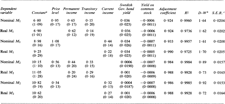
^a Numbers in parentheses are standard errors.

^b Durbin–Watson statistic.

^c Standard Error of the Regression.

The poor performance of the government bond yield is a direct reflection of the controls on bond issues and holdings by the central bank. As suggested on p. 308 above these restrictions make the bond rate an inadequate measure of the opportunity cost of holding money. Due to lack of data, we were unable to test the hypothesis that trade credits are a closer substitute to money. With respect to the yield on common stock, it might be that the current yield is a poor indicator of the anticipated yield as seems to be true for the U.S.²¹

Monetary Policy

Monetary policies in a closed economy are usually assumed to operate either through interest rates or directly on prices and output. In a small economy on a fixed exchange rate, however, we have seen that both the structure of interest rates and the price level will be dominated by foreign influences. In Sweden even the rate of production is dependent on the international business cycle as we can see from Figure 13.2, although government policies undoubtedly can affect both the timing and amplitude of the Swedish fluctuations within narrow limits.

To test whether monetary policy has influenced income to a significant extent, or whether the stock of money is demand determined, a method developed by Sims²² was applied to Swedish money and income data. The procedure is designed to determine temporal ordering of time series, so the well-known caveats regarding the relationship between temporal precedence and causality must be kept in mind.

Table 13.7 shows the results of regressions relating log-changes in money (M₁) and nominal income with various leads and lags. Assuming that the errors are normally distributed, the F-statistics in the last column indicate that the future values of money in the income regression are marginally non-zero (row 7) and that the future values of income in the money regression are not significantly different from zero as a group (row 4). Thus, applying Sims’ criterion we conclude that income changes have preceded changes in money in Sweden during the sample period. These findings are consistent with the view that the demand for money has determined the stock in existence, and they do not support the hypothesis that monetary policy has had a systematic effect on the flow of income at least as far as this effect is anything but immediate.²³

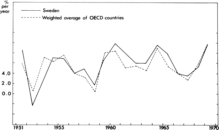
Figure 13.2. Yearly Growth Rates of Industrial Production.

Table 13.7 Money-Income Regressions^a

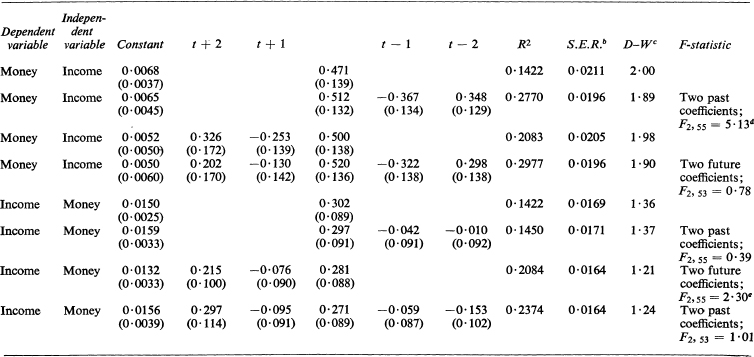
^a Variables expressed as log-changes.

^b Standard Error of the Regression.

^c Durbin-Watson statistic.

^d Significant at 95 per cent level.

^e Significant at 90 per cent level.

The coefficients of the current and lagged values of the income variable in Table 13.7 are interesting in that the current value alone contributes virtually as much as the sum of all periods taken together. This suggests that the money-income relationship has been concurrent on the average throughout the fifties and sixties. It is also a reflection of the fact that the current income variable performed as well as the permanent income series in the demand equations of the previous section.

In an economy with both traded and non-traded goods there might be an impact of monetary policy on the relative price of these classes of goods. In a full-employment theoretical model, an expansionary monetary policy would cause an excess demand for both types of commodities. The demand for traded goods would be met by increased imports or decreased exports but in the non-traded sector the excess demand would have to be eliminated by a price increase. Thus if this effect was powerful enough we should be able to observe a positive relationship between monetary expansion and the relative price of non-traded goods. Figures 13.3(a) and (b) show the behaviour of these variables during the 1960s.^{24, 25} It is not possible to discern a relation between them,²⁶ so this influence of monetary policy does not appear to have been important in Sweden.

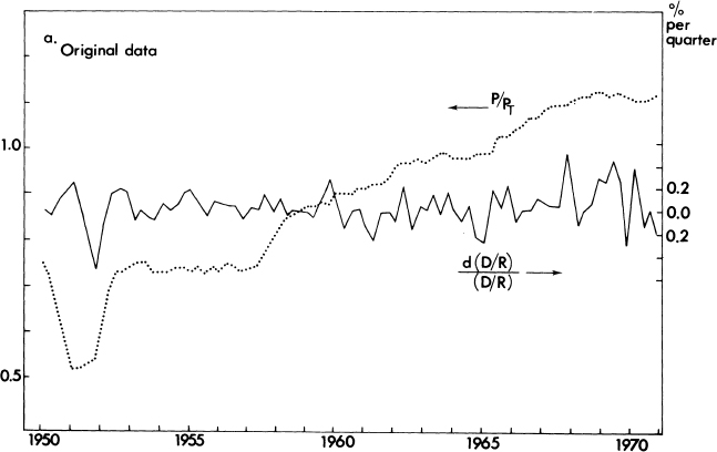
Figure 13.3(a). Monetary policy and the relative price of non-traded goods.

Figure 13.3(b). Monetary policy and the relative price of non-traded goods.

MONETARY EQUILIBRIUM AND THE BALANCE OF PAYMENTS

In the previous sections we have shown how the usual channels of monetary policy are not open to a small economy in a fixed exchange rate system. Neither commodity prices nor interest rates appear to be sensitive to domestic monetary forces unless these are in accord with world market conditions. In Sweden it appears that the rate of output is also influenced little by the money stock. The demand for money will determine the actual volume in existence because the central bank effectively assures a perfectly elastic supply by its commitment to the fixed exchange rate regime. As we mentioned above, the division of the backing of the monetary base between international reserves and domestic assets will become the variable under central bank control. In this section we shall present some evidence bearing directly on this particular implication of the monetary approach. Specifically, we shall compute a predicted time path for the balance of payments and compare that with the actual reserve flow during the period.

Following Johnson²⁷ we can derive a reserve flow equation from (1) by equating money demand and supply. Letting a g stand for the relative growth rate of the variable appearing as a subscript we get:

Equation (6) implies that the equilibrium rate of reserve inflow will be equal to the desired growth rate of money demand adjusted for changes in the multiplier and central bank credit creation. By using the empirical demand functions estimated above, we can arrive at a predicted reserve flow by substituting the predicted g_MD from these equations.²⁸

Figures 13.4(a) and (b) show the actual and predicted percentage reserve flows for two different demand functions for money (corresponding to rows 3 and 7 of Table 13.6 respectively). The obvious similarity of the series is illustrated quantitatively in Table 13.8 where some summary statistics of the comparison are reported.

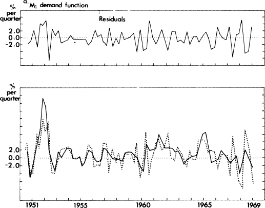
Figure 13.4(a). Actual (solid line) and predicted (dotted line) reserve flows, M₁.

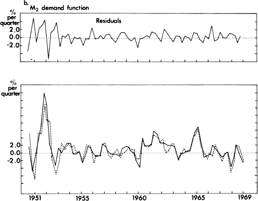
Figure 13.4(b). Actual (solid line) and predicted (dotted line) reserve flows, M₂.

Table 13.8 Comparison of Actual and Predicted Reserve Flows: 1950–III to 1968-1V.

Definition of money	M1	M2
Squared correlation coefficient	0.5012	0.7642
Regr. coeff. of actual on predicted	0.5913	0.8972
Mean absolute error	0.0212	0.0108
Fraction of error due to difference of regr.
coeff. from unity	0.3223	0.0401
Fraction of error due to residual variance	0.6715	0.9436

The high correlations between the actual and predicted reserve flow series strongly support the monetary interpretation of balance-of-payments adjustments. The variance left unexplained in the M₁ case can be attributed largely to substitution between demand and time deposits not captured in the empirical demand function,²⁹ which could also explain the possible presence of serial correlation in the residuals from a regression of the actual on the predicted balance of payments.³⁰

The difference of the regression coefficients from unity as indicated in Table 13.8 could be an indication of a lagged response of reserve flows to the forces involved in the predicted (desired) series. If an adjustment equation of the type

was relevant, then a lagged relationship between (R/H)g_R and [(R/H)g_R]^D would be appropriate and take the form

With our current coefficient estimate of 0.59 for M₁ this would mean a lag pattern of 0.24, 0.10, 0.04, 0.02, 0.01 for the first through fifth lag indicating an average lag of about two months. The M₂ coefficient of 0.90 would similarly imply an average lag of one and a half weeks.

Before too much is made of these calculations, however, we must point out that if there is a lag in the adjustment so that desired reserve flows will not be fulfilled, then this should be integrated into the specification and estimation of the money demand functions in which case the ‘true’ parameters could be found. This problem will be left for future research.

Before we conclude the direct examination of the balance of payments, we must deal with an alternative to the monetary interpretation of our results. Sceptics of the monetary approach argue that the close inverse relationship between reserve flows and domestic credit creation is the result of sterilisation policies of the central bank. An autonomous reserve inflow will, according to this view, cause the central bank to contract domestic credit by the same amount in order to prevent the balance-of-payments surplus from affecting the money supply. This interpretation is implausible for several reasons. Firstly it implies an extraordinary stability of the central bank’s behaviour with respect to policy formation. Secondly it implies that the sterilisation is always of a magnitude consistent with the demand for money, since with prices, interest rates and output determined by exogeneous forces, the money market must be equilibrated through either reserve flows or domestic credit creation. It seems far-fetched to assume that this kind of rule is followed by the Swedish central bank. Nevertheless, the possible simultaneous relationship between the two variables suggests that estimation procedures should take it into account. As a suggestive illustration we shall therefore present some results of simultaneous estimation of the system:

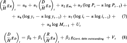
where (7) is the reserve flow equation (6) with the short-run demand for money function (4) of p. 310 substituted for (g_MD)^D, and (8) is a government policy reaction function. The latter assumes that open market operations are dictated by the change in international reserves (the sterilisation hypothesis) and the change in government debt outstanding (on the hypothesis that the central bank is a large source of finance for the government).

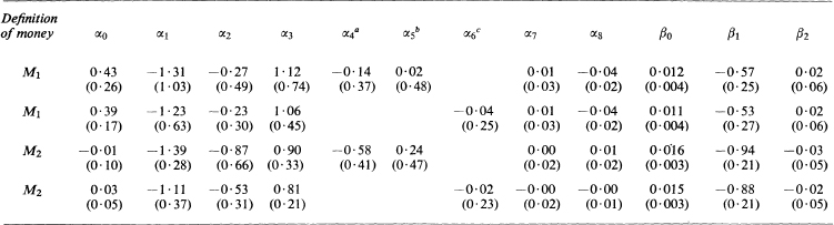
The two-stage least squares estimates of the parameters given in Table 13.9 indicate first of all that the specification of the central bank reaction function is inadequate in that the government financing variable fails to be significant. This is likely the result of short-run instability of the central bank’s policy response due to the existence of many alternative targets. Experiments with yearly data did produce a significantly positive β₂ consistent with the long-run need for deficit financing through the central bank.

As far as the reserve flow equation is concerned, our conclusions still hold, judging from the α₁, α₂, and α₃ estimates which are not significantly different from their a priori values of – 1 (for the first two) and + 1. The income- and interest-rate coefficients are estimated with such poor precision that they are not significantly different from the estimates in the demand functions of Table 13.6 above even though the point estimates are contrary to expectations.

In conclusion it does not appear that the sterilisation hypothesis offers a very plausible alternative to our explanation of reserve flows. The monetary approach has passed our tests both as far as its underlying view of the world is concerned and in its implications with respect to the balance of payments.

Table 13.9 Two-stage Least Squares Estimates of the Parameters in (7) and (8)

^a Permanent income.

^b Transitory income.

^c Current income

REFERENCES

Agmon, Tamir, ‘Country Risk: The Significance of the Country Factor for Share-Price Movements in the United Kingdom, Germany, and Japan’, The Journal of Business, 46 (January 1973), 24–32.

Agmon, Tamir, ‘The Relation Among Equity Markets: A Study of Share Price Co-movements in the United States, United Kingdom, Germany and Japan’, Journal of Finance, xxvii (September 1972), 839–55.

Argy, Victor, and Hodjera, Zoran, ‘Financial Integration and Interest Rate Linkage in the Industrial Countries’, International Monetary Fund Staff Papers, xx (March 1973), 1–77.

Branson, William H., Financial Capital Flows in the U.S. Balance of Payments (Amsterdam, North-Holland, 1968).

Branson, William H., and Hill, Raymond D., Jr, Capital Movements in the OECD Area. An Econometric Analysis. OECD Economic Outlook Occasional Studies (Paris, OECD, December 1971).

Chow, Gregory, ‘On the Long-Run and Short-Run Demand for Money’, Journal of Political Economy, lxxiv (April 1966), 111–31.

Cooper, Richard N., ‘Towards an International Capital Market?’, North American and Western European Economic Policies, Proceedings of a Conference held by the International Economic Association, edited by Charles P. Kindle-berger and Andrew Shonfield (New York, St Martin’s Press, 1971), 192–208.

Genberg, A. Hans, ‘Aspects of the Monetary Approach to Balance of Payments Theory: An Empirical Study of Sweden’, unpublished Ph.D. dissertation, University of Chicago (1973).

Genberg, Hans, ‘The Concept and Measurement of the World Price Level and Rate of Inflation,’ Discussion Paper, GIIS-Ford Foundation International Monetary Research Project (Graduate Institute of International Studies, October 1974).

Grassman, Sven, Valutareserven och Utrikeshandelns Finansiella Struktur. Bilaga till betalningsbalansutredningens betänkande. SOU 1971: 32. (Stockholm, Finansdepartementet, 1971).

Grubel, Herbert G., ‘Internationally Diversified Portfolios’, American Economic Review, lviii (December 1968), 1299–1314.

Hultcrantz, Gerhard, ‘Prognos och Ekonomisk Verklighet’, Svensk Finanspolitik i Teori och Praktik, edited by Erik Lundberg et al. (Stockholm, Bokforlaget Aldus, 1971), ch. 4.

Johnson, Harry G., ‘The Monetary Approach to Balance of Payments Theory,’ Journal of Financial and Quantitative Analysis, vii (March 1972), 1555–72.

Laffer, Arthur B., and Zecher, J. Richard, ‘Some Evidence of the Formation, Efficiency and Accuracy of Anticipations of Nominal Yields’, University of Chicago (January 1973), mimeographed.

Organisation for Economic Co-Operation and Development, Main Economic Indicators, Historical Statistics (Paris, OECD, 1970).

Scott, Ira O., ‘The Euro-dollar Market and Its Public Policy Implications’, Economic Policies and Practices, paper no. 12, prepared for the Joint Economic Committee, 91st Congress, 2nd Session. (Washington, U.S. Government Printing Office, 1970).

Sims, Christopher A., ‘Money, Income, and Causality’, American Economic Review, lxii (September 1972), 540–52.

¹ This chapter is based on my Ph.D. dissertation with the same title at the University of Chicago. I would like to express my gratitude to my advisers, Professors H. G. Johnson, A. B. Laffer, and J. R. Zecher, for their guidance and encouragement during the preparation of the dissertation.

² This route is also followed by the project LINK.

³ OECD (1970)

⁴ Exchange rate changes were in other words treated as breaks in the price index series affecting only the quarter of the exchange-rate change.

⁵ In terms of the notation in (1) the F-ratio is computed as:

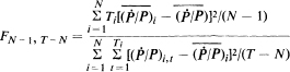
where is the mean rate of inflation in country i, N is the number of countries, N T_i is the number of observations on country i, and

⁶ Austria, Belgium, Italy, Japan, Norway, Portugal, Sweden, Switzerland, and U.S.A.

⁷ The degrees of freedom were 8,153 and 7,136 respectively.

⁸ Atlanta, Baltimore, Boston, Chicago, Cincinnati, Cleveland, Detroit, Los Angeles, New York, Philadelphia, Pittsburgh, San Francisco, Seattle, St Louis, and Washington, D.C.

⁹ The definition of the world rate of inflation used here was simply the arithmetic average of the other fifteen countries mentioned above plus Canada. The concept and measurement of the world rate of inflation are investigated in Genberg (1974).

¹⁰ See, for instance, Grubel (1968).

¹¹ See Branson (1968), and Branson and Hill (1971).

¹² Agmon (1972), and Agmon (1973).

¹³ ibid. Specific country factors were found, but they were not such that international diversification could improve on efficient portfolios based entirely on U.S. stocks.

¹⁴ Adjusted for dividend payments and capital changes, and converted into $U.S. by the appropriate spot exchange rate.

¹⁵ Scott (1970).

¹⁶ Cooper (1971).

¹⁷ Argy and Hodjera (1973).

¹⁸ As an example of the speed and size of the possible reserve loss, consider the following example from Grassman (1971), p. 13 (see also his footnote on the same page): suppose that export and import payments each are of the magnitude 36,000 million Swedish Kronor per year (these are approximately the correct figures for 1970), and suppose they are evenly distributed over each week. Then a two-week lead payment for exports and the same lag for imports implies a reserve loss of 3,000 million kr. This should be compared with the average (for 1970) net international reserve holding of the central bank of approximately 3,300 million kr.

¹⁹ Chow (1966).

²⁰ The coefficients in the long-run function are also in accordance with estimates of a long-run demand function carried out on yearly data. See Genberg (1973), ch. 4.

²¹ See Laffer and Zecher (1973), pp. 10 and 11.

²² Sims (1972).

²³ These results could also be consistent with a potent monetary policy if it was always perfectly anticipated.

²⁴ The relative price is actually the ratio of a consumer price index to a traded-goods index. This will behave as the theoretically desirable ratio under general conditions. The monetary variable is the relative change in the D/R ratio which will increase as a result of expansionary monetary policy and vice versa.

²⁵ Figure 13.3(b) shows the price ratio in detrended form in an attempt to allow for different rates of technical progress in the two sectors. Slower technical change in the non-traded goods sector would imply an increasing relative price of non-traded goods over time.

²⁶ This conclusion was also supported by the regression analysis allowing for lags in the adjustment.

²⁷ See ch. 6.

²⁸ Using the actual values of g_m and () might be subject to criticism. As a justification we argue that in the case of the multiplier, the variables determining it are exogeneous to the system we are considering and can therefore be safely ignored when we test the predictive ability of the model. In forecasting, of course, these variables must be specified in advance.

The simultaneous equation problems associated with the use of the actual value of the credit creation variable will be discussed at some length below.

²⁹ The different results as between the M₁ and M₂ predictions derive from the relatively erratic behaviour of the M₁ money multiplier during some periods in the sixties. This stems from the large changes in the currency-demand deposit ratio during quarters immediately before and after major changes in indirect taxes and is witnessed by the importance of the currency ratio as a proximate determinant of changes in M₁ during the sixties (see Genberg (1973), ch. 3, table 4, row 3). For M₂ the currency and time deposit ratios work in the opposite directions with a smaller net effect (ibid., table 4, row 6).

The significance of the currency ratio behaviour in the present context is that it points to the instability of the M₁ function as specified on page 310 above relative to the M₂ function.

³⁰ The Durbin–Watson statistic is 1.63 which is in the uncertain region at the 95 per cent level. The same regression but with the M₂-based prediction yielded a Durbin-Watson statistic of 2.06, indicating no significant serial correlation there.