International Reserve Flows and Money Market Equilibrium
The Japanese Case1
DONNA L. BEAN
INTRODUCTION
The monetary approach to the balance of payments attributes a significant role in the international adjustment process to monetary variables.2 The model predicts that reserve accumulation is positively related to the rate of growth of domestic income and negatively correlated with the rate of domestic credit expansion. Some of the policy implications which follow from these results contradict the standard Keynesian analysis. The monetary approach implies that the central authorities can exercise some degree of control over the level of international reserves by manipulating the composition of the money supply base through adroit credit creation policies. Alternatively, this framework stresses the role of discretionary monetary policy in sterilising the impacts of the flows in the balance-of-payments accounts.
THE MODEL
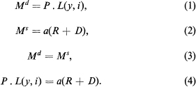
The model is derived by applying the basic assumption that the money market is always in equilibrium. The following notation is used in the model:
| a | = | money multiplier, |
| H | = | high-powered money, |
| R | = | central authorities’ international reserves, |
| D | = | domestic credit issued to the government or commercial banks which is due to the central bank, |
| i | = | interest rate, |
| P | = | price level, |
| y | = | real income. |
The demand for money is described by equation (1), the supply of money by equation (2), and the money market equilibrium condition by equation (3) or equivalently by (4).
Differentiating equation (4) logarithmically yields:

where ny and ni are, respectively, the elasticity of the demand for real cash balances with respect to income and the rate of interest. Solving for [R/(R + D)] d log R:
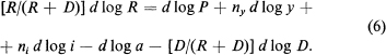
Equation(6) is estimated in the following form:
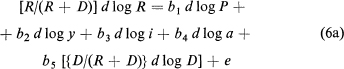
where e is the stochastic disturbance.
The coefficients for the income and interest-rate variables are the elasticities of the demand for money with respect to these particular parameters. Previous statistical work implies that b2 should be of the order of magnitude of unity, and b3 should be a small negative number. Since it is assumed that there is no money illusion the price coefficient should be +1. The theory predicts that the elasticity of the dependent variable with respect to the money multiplier and the domestic component of the base is –1.
If we let r = R/(R + D) which implies that D/R = (1 – r)/r then equation (6) can be written as:
![]()
Equation (7) is estimated in the following form:
![]()
Estimations for the two forms of the equation are presented.
COMMENTS ON THE OBSERVATION PERIOD
This study examines the Japanese economy for the period 1959–70. The selection of Japan was arbitrary, and it may seem an unlikely candidate for a model applying what is often viewed as a small-country assumption—the price-taking hypothesis (this subject will be discussed further in a subsequent section). The availability of data played some role in the selection of the time interval.3 By 1956 the recovery of pre-World War II levels of industrial production and productivity were achieved. The pre-war per capita income level was attained in 1954. These facts indicate that many of the problems associated with reconstruction after World War II had been eliminated. Inclusion of data subject to the vagaries of post-war occupation and rebuilding seemed undesirable.
The sensational economic growth and radical structural changes which characterise the observation period were linked with growing surpluses in the international accounts. This high growth rate was sustained in part by attractive capital and labour arrangements which stimulated investment. Policies invited depreciation allowances and retained earnings which enabled the authorities to pursue a restrained monetary policy without provoking a severe excess demand for borrowings.
By 1969–70 the prolonged growth period created pressure for appreciation of the exchange rate or a de facto parity adjustment through removal of remaining tariff barriers. From 1950–70 the yen was pegged at 360/U.S.$. However, in 1950 the currency was overvalued at this rate, and extensive import controls were used to support this parity. Exchange rate alignment occurred throughout the period by the gradual relaxation of these regulations. These adjustments failed to capture all of the effective appreciation of the yen, and by 1969 the Japanese currency was believed to be greatly undervalued at this exchange rate.
The commercial banking sector is stringently administered by the central bank; in addition, during the 1960s, the corporate business sector had to rely on the banks for external financing due to the under-developed structure of alternative markets. These structural aspects of the banking sector resulted in a cartel of commercial banks in which credit was not regulated solely by means of price competition. Through this medium of the monopoly position of banks in issuing debt instruments, the authorities maintained strict control over the variables affecting money supply.
Two interrelated aggregative financial aspects accompanying this growth are noteworthy.4 Firstly, the level of reserves was apparently a target variable during part of the decade. During this period, the trade balance fluctuated by more than $1 billion (over half the stock of reserves). Secondly, since fiscal policy was balanced over the long run with only a minor increase in government debt, this phenomenon was apparently achieved through discretionary monetary policies.
Indeed, monetary policy evidenced cyclical tendencies in the 1950s and 1960s and it has been suggested that four declines in productivity during this period were induced by restrictive governmental policy aimed at deterring reserve flows.5 In sum the authorities were utilising their capacity as domestic credit creators to control reserve flows. The monetary approach to the balance of payments provides the theoretical background which explains why this policy was effective.
THE PRICE VARIABLE
The price-taking assumption refers specifically to price equilibration in the tradeable goods sector and in the long-run steady state. There is no readily available index for Japan for traded goods. A composite of the export and import price indices is especially inadequate in this country’s case for two reasons. It is well known that Japan made price concessions in an attempt to increase market share. In addition, the import price index is heavily weighted by raw minerals, unfinished goods, and unprocessed agricultural products. Consumer goods prices are a biased estimator of traded goods because of the high services content. Wholesale prices do not include services but retain non-tradeables such as heavy construction—a sector in which costs have risen rapidly.
Price index movements for Japan during this period are quite diverse. The Japanese consumer price index (CPI) rose twice as fast as the United States CPI from 1953 to 1970. This relative increase cannot be explained by the application of a monopolistic pricing situation to Japan. At the same time, the change in the wholesale price index (WPI) is less than that for the comparable United States index. Meanwhile, the export price index fell in absolute terms from 1957–69.
One study of several nations concludes that the discrepancy between the CPI and WPI is a function of the rate of growth of output per capita; the more rapid the increase in productivity the greater this difference.6 This greater upward movement in the CPI can be traced to real wage gains which are rapidly translated into price increases in the non-traded goods sector. McKinnon suggests that wholesale price indices, under fixed exchange rates, should be correlated due to international arbitrage, especially if the data are converted into dollar terms. More specifically, he asserts that an appropriate traded-goods index should rise somewhat less than the wholesale price index.7
The empirical exception to WPI covariance is Japan; the absolute level of the WPI remained low relative to the rest of the world. McKinnon converts the yen indices into dollar terms using the 360/U.S.$ exchange rate. However, it has been suggested that the yen appreciated and the removal of import barriers and quotas was the mechanism used to implement parity adjustments.
In order to measure the extent of these changes in exchange controls the following method was employed. Data are published on the black market exchange rate. Although there is a premium assessed to buyers for the privilege of being able to obtain dollars which they otherwise could not procure (i.e., the yen is under-valued in relation to the rate which would prevail in an unrestricted market), this premium is assumed to be constant throughout the period. Accordingly, the adjusted price indices consist of the raw data multiplied by a black market exchange rate factor.
Summarily, adjustment by a crude measure for conversion of yen into dollars results in a price series which generally supports the price-taking hypothesis. The collinearity between the U.S. WPI and Japanese WPI is more striking when the Japanese prices are adjusted by the changing free market rate; this supports McKinnon’s statement concerning international arbitrage.
Having established that the price-taking hypothesis is applicable, it is still necessary to select a price series which represents the measure used by the public to deflate their nominal money balances. Export and import price indices do not appear to meet this criterion explictly. McKinnon’s analysis supports the notion of using the wholesale price index. However, this index has at times been a target variable of the Japanese policy-makers; this interference makes the index a less appealing price-level proxy. The consumer price index remains; this measure is most frequently utilised in money demand estimations. Both the WPI and CPI are incorporated in the statistical analysis.
Assuming that the free market in yen is not extensive, there is reason to question the appropriateness of using the adjusted indices for the price variable. If it is the case that access to the market is possible on a small scale, then consumers must view this price as the marginal price, for otherwise they would exercise the option of trading in this market in order to capture the rents available. The existence of this market suggests that the free rate represents the shadow price. If it did not, then the opportunities for arbitrage indicate a state of disequilibrium; since all markets are assumed to clear, the price index adjusted by the free market rate must represent the effective price deflator.
RESULTS
The data8 were seasonally adjusted. Two further pieces of information were generated from these data series—the money multiplier and velocity. The multiplier is relatively unstable. Velocity is a reasonably stable function—particularly for the narrow definition of the money stock. This observed stability supports one assumption underlying the model.
The results of the estimations are presented in Tables 14.1 and 14.2 for both forms of the equation. In general, form 1 is statistically more significant, yielding higher R2s, bètter Durbin–Watson statistics, and larger t-statistics.
All of the estimated coefficients have the predicted sign. The income elasticity is consistently smaller than unity.9 The use of the Japanese discount rate results in a larger interest rate elasticity than when the United States treasury bill rate is used, but the difference is not statistically significant. The money multiplier is not appreciably different from the predicted value of unity.10 Estimates of the elasticity of the domestic component of the base are smaller than the expected magnitude.11
Looking at Table 14.1, it is clear that the confidence levels of the coefficients are greater when the U.S. treasury bill rate is used (see columns 1 and 2, 5 and 6). In order to isolate the impact of alternative price indices the results using the treasury bill rate will be compared.
Over all, the consumer price index performs better than the wholesale price index. For the latter index serial correlation (as indicated by the Durbin–Watson statistic) may result from the authorities’ policy of controlling wholesale prices during certain sub-periods.
Adjusting the price index by the free market rate has two effects. Firstly, the coefficient of the consumer price index more closely approximates unity (see Table 14.1, columns 1 and 5). In addition the statistical reliability of the WPI estimates improve (see Table 14.1, columns 3 and 7).
CONCLUDING REMARKS
The empirical analysis of Japan presented in this study strongly supports the theses of the monetary approach and suggests that it is a useful framework for analysing these phenomena.12 Moreover, it is obvious that statistical estimations are sensitive to the definitions of the variables which are employed. The nominal balances and income deflator are more appropriately specified by adjusting for the exchange rate since money demand can be satisfied in either the domestic or the foreign sector.
The theory implies that through discretionary credit-creation policies the authorities can minimise the impact of reserve flows on the economy. Alternatively, given a particular rate of growth of money demand, the authorities can peg reserves by manipulating the domestic component of the base. From 1964–6 international reserves stabilised around $2 billion. Demand deposits did not reach their fourth-quarter 1963 level until 1966; because of the disparity in the data series (see footnote 8), it is impossible to determine the extent of measurement bias and actual reduction in the rate of growth of money demand. However, it is clear that the central bank did control the composition of its assets by varying the rate of growth of domestic credit so that international reserves were not depleted.
Table 14.1 Form 1, Equation (6a)
(R/(R+D))d log R = b1d log P + b2d log y + b3d log i + b4d log a + b5[{D/(R + D)}d log D] + e Quarterly: 1959–70 Price Index and Interest Rate Variablea
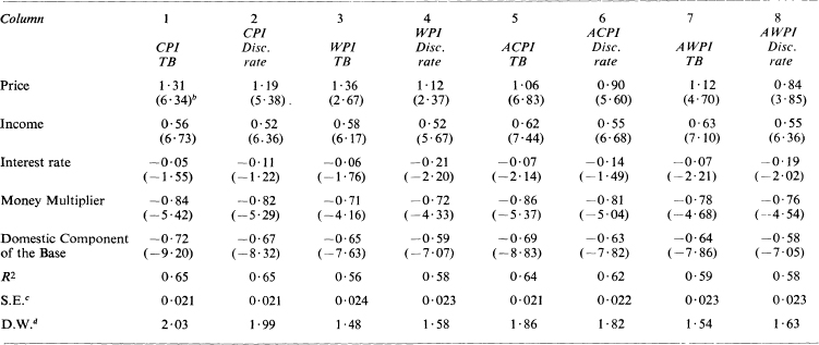
a The price indices are for consumer or wholesale prices. An ‘A’ preceding the index abbreviation indicates those series adjusted by the exchange rate. The United States treasury bill rate is series ‘ТB’ and ‘Disc. rate’ represents the Japanese discount rate.
b t-statistic.
c Standard error of the regression.
d Durbin–Watson statistic.
Table 14.2 Form 2, Equation (7a)
(d log R=b1d log P + b2d log y + b3d log i + b4d log a + b5[{(1—r)/r}d log D] + e
Quarterly: 1959–70 Price Index and Interest Rate Variablea
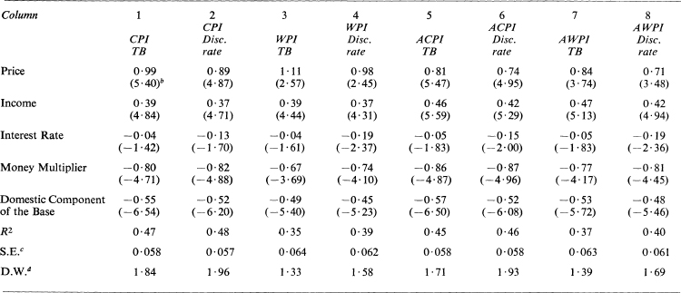
a The price indices are for consumer or wholesale prices. An ‘A’ preceding the index abbreviation indicates those series adjusted by the exchange rate. The United States treasury bill rate is series ‘ТB’ and ‘Disc. rate’ represents the Japanese discount rate.
b t-statistic.
c Standard error of the regression.
d Durbin–Watson statistic.
1 This chapter is an excerpt from research supported by a National Science Foundation grant when the author was an undergraduate at the University of Chicago. The research was advised by Richard Zecher. The author also benefited greatly from discussions with Jacob Frenkel, Rudiger Dornbusch, and Robert Z. Aliber.
2 See Johnson (ch. 6) for an elaboration of the monetary approach.
3 Quarterly observations for 1957 and 1958 were sampled out as preliminary estimations demonstrated that poorer Durbin–Watson statistics resulted when this period was included.
4 See Michael W. Keran, ‘Monetary Policy and the Business Cycle in Postwar Japan’, in Varities of Monetary Experience, ed. by David Meiselman (Chicago, University of Chicago Press, 1970), and Robert Z. Aliber, ‘Japanese Growth and the Equilibrium Foreign Exchange Value of the Yen’, (mimeo).
5 Keran, op. cit.
6 Ronald I. McKinnon, ‘Monetary Theory and Controlled Flexibility in the Foreign Exchanges’, Essays in International Finance, no. 84 (Princeton, Princeton University Press, 1971).
7 ibid, p. 22.
8 Data were primarily obtained from a computer tape of International Financial Statistics (IFS). Various issues of the Economic Statistics Monthly (ESM) published by the Bank of Japan were also employed. Free market exchange rates are from Pick’s Currency Yearbook.
Reserves are the foreign assets of the ‘monetary authorities’ which includes the Bank of Japan, the Foreign Exchange Fund, and Treasury IMF accounts (line 11, IFS). Beginning in 1964 Exchange Fund foreign exchange deposited with domestic commercial banks is not reported in this figure and is subsequently recorded as claims on commercial banks. The ‘Monetary Survey’ table in the ESM provided an adjustment factor for this phenomenon. It appears that 110 billion yen represents these deposits for the period prior to 1964; this figure was deducted from the data points for 1959–63.
High-powered money is line 14, IFS; those are funds expressly designated as reserves by the monetary authorities. (Note: there is reason to suspect this particular datum due to the close relationship between the central bank and the commercial banks. Alternative definitions which include the combined reserves of these institutions are not included in this analysis.) The domestic backing of the base is the difference between lines 14 and 11; this removes the noise generated by the ‘other net’ account. No distinction was made between domestic credit issued to the government or the commercial banks. Essentially, the balance sheet of the central bank was collapsed to two accounts so that the identity, H = R + D, is operable.
Money is defined in a broad sense to include currency, savings deposits, and time deposits (lines 34 and 35, IFS). Different accounting practice was adopted in 1964; yen balances of non-residents (previously included in demand and time deposits) were transferred to the category foreign liabilities. This had a substantial effect on the third item included in the money stock. Unfortunately, it is not possible to isolate the size of these deposits. As the model is expressed in percentage changes, this difficulty was circumvented by sampling out the quarter in which the transformation occurs.
Income is represented by the Gross National Product. This figure is a quarterly level not projected to an equivalent annual flow.
The only series of interest rates obtainable from the tape is the discount rate. As this rate was comparatively stable, and is a discretionary policy variable, it is a less than optimal indicator of the movements in the prices of financial assets. Using the perfect capital market assumption, the U.S. treasury bill rate (line 60b, IFS) was also employed for the cost of capital variable. The last variable, commodity prices, are lines 63 and 64, IFS.
9 A permanent income series should produce a larger magnitude. When the regression was run for semi-annual data, the income elasticity rose to approximately 0.70.
10 Using the narrow definition of money does not significantly alter the level of statistical significance. The only noteworthy change is that the coefficient of the money multiplier falls, but this is the expected result.
11 As mentioned in footnote 8, high-powered money may be more appropriately measured by a definition which includes a portion of the deposits of the commercial banking system. If it is true that increases in foreign reserves were hidden in the commercial banks’ accounts, then the elasticity of reserve flows with respect to domestic credit expansion should increase if the estimation was run for this alternative measure of high-powered money.
12 Criticism of this formulation might be centred on the assumption that the money market clears instantaneously. However, it should be noted that this model is geared to long-run analysis and acknowledges the transitory periods of stock adjustment. Regressions involving yearly data may yield estimates of the coefficients which more precisely reflect the postulated magnitudes.