Chapter 9
The Monetization the Climate Science
9.1 Introduction
The Internet era dawned on us with the hope of infinite transparency, great efficiency, and unprecedented prosperity. Much of the predictions have come true, but in the wrong direction. Clearly, Information age has monetized everything and every bit of indecency and act of immorality has cashed in with great reward. They will eat worms, hot peppers, rotted fish, road kills, live octopus, you name it – all to maximize views that translate directly into financial gains. While these YouTubers gain notoriety (which they do not mind because any publicity is good publicity), few notice that Jeff Bezos (Amazon), Mark Zuckerberg (Facebook), Larry Page and Sergey Brin (Google) are only the polished version of YouTubers. Even fewer realize that every scientist or researcher is focused on maximizing monetary gain. Knowledge is nothing unless it fetches financial gains. Similarly, as long a concept is monetized, there is no concern about it being right or wrong.
Ever since the oil embargo of 1972, the world has been gripped with the fear of ‘energy crisis’. U.S. President Jimmy Carter, in 1978, told the world in a televised speech that the world was in fact running out of oil at a rapid pace – a popular Peak Oil theory of the time – and that the US had to wean itself off of the commodity. Since the day of that speech, worldwide oil output has actually increased by more than 30%, and known available reserves are higher than they were at that time. This hysteria has survived the era of Reaganomics, President Clinton’s cold war dividend, President G.W. Bush’s post-9–11 era of ‘fearing everything but petroleum’ and today even the most ardent supporters of petroleum industry have been convinced that there is an energy crisis looming and it’s only a matter of time, we will be forced to switch no-petroleum energy source.
Almost simultaneous to the energy crisis hysteria, global warming has been a subject of discussion. It is thought that the accumulation of carbon dioxide in the atmosphere causes global warming, resulting in irreversible climate change. Even though carbon dioxide has been blamed as the sole cause for global warming, there is no scientific evidence that all carbon dioxides are responsible for global warming. This is despite the claim of vast majority of scientists that the global warming is all about carbon (Crooks, 2018). We have seen in previous chapters, scientists have either started off on false premises or have been ignoring crucial flaws of New Science to justify their assertion that climate change is about carbon dioxide.
The IPCC 5th Assessment Report (AR5) assessed carbon budgets for various levels of warming in billions of tonnes of carbon (GtC) or of carbon dioxide (GtCO2) based on projections of global nearsurface air temperature change, which referred to as ‘global-tas’1, from complex Earth System Models (ESMs. In general, climate modelling studies use global-tas, whereas observational records typically combine nonglobal coverage of near-surface air temperature over land with sea-surface temperature (SST) over oceans. Richardson et al. (2018) avoid using the term global average temperature with ‘carbon budget’. This usage of ‘carbon budget’ essentially expresses temperature in terms of quantifiable action item. Built-in in this analysis is the outcome that carbon tax can solve problems that are perceived to be due to greenhouse gas effects. Richardson et al. (2018) list three main factors that contribute to differences in ‘global average temperature’ change between globaltas and observational records. First, there are regions with missing data that may not warm at the global mean rate. As an example, they cite the cases of the Arctic, which is now rapidly becoming warmer and wetter (Boisvert and Stroeve, 2017) but the fate of which could not be identified with temperature data that are sparse at best (Cowtan and Way, 2014). Secondly, under CO2-driven global warming, modelled near-surface air temperatures warm more than the values of sea-surface temperature (SST), as pointed out by Richter and Xie (2008). Thirdly, data providers must decide how to account for changes in sea ice. There may be a change from reporting estimated near-surface air temperatures to SSTs where ice has retreated. In the HadCRUT4 dataset2 (Morice et al., 2012), this approach probably results in an artificially low reported warming compared with the air warming due to features of the normalisation procedure. Clearly the lack of data cannot be replaced by desired outcome without sacrificing the scientific validity of the model. Richardson et al. (2018) called it ‘masking’, and the other two factors together as ‘blending’, specifically ‘air-sea blending’ and ‘sea-ice blending’. One early study accounted for the masking and air-sea blending issues (Santer, 2000), and some studies have accounted for masking but this is not universal, although few scintists have raised the issue of misrepresentation. Recently, it was shown that over 1861–1880 to 2000–2009, modelled global-tas increased 24% more than a Had CRUT4 like blended-masked estimate (Richardson et al., 2016). Instead of attributing this discrepancy to the misrepresentation of the science underlying the climate change phenomena, Richardson et al. (2016), concluded that current observed temperature records should exceed 2 C later than global-tas, implying a larger carbon budget if compliance were assessed using one of them. Richardson et al. (2018) simply extended this work by
- reporting results to 2099,
- calculating carbon budgets using IPCC techniques,
- accounting for realistic potential future data coverage and
- applying blending and masking to a low-emission scenario.
The focus has been on the scenario that lowers emission scenario based on various policy impositions. Because no new data was added and because no further improvement is scientific description was available, blending-masking biases continue to exist without any means to determine what caused the discrepancy. For instance, the blending-masking bias under transient warming with 2000–2009 data coverage was estimated to be 15% instead of 24% (Richardson et al., 2016). Furthermore, with strong mitigation sea-ice cover would be expected to stabilise before 2100, suppressing the future sea-ice blending bias (Swart et al., 2015). In addition, the long-term warming pattern may differ from the historical pattern, leading to a different effect of coverage bias (Armour et al., 2013; Andrews et al., 2015; Held et al., 2010).
A very large amount of pseudo-science is already afoot on all aspects of the issue of climate change. Much of it is used to divide – if not aimed at dividing in the first place – public opinion over whether nature or humanity is the chief culprit. The crying need for a serious scientific approach to be taken has never been greater. On this note, paraphrasing Albert Einstein, it can truly be said that the system that got us into the problem is not going to get us out. Absent a comprehensive characterization of CO2 and all its possible roles and forms, any attempt to analyze the symptoms of global warming or design a solution must collapse under the weight of incoherence if it is based on univariate correlations, or even correlations of multiple variables, and assumes that the effects of each variable can be superposed linearly and still mean anything. The absurdity is so well known that one popular graph on the Internet depicts a strictly proportional increase in incidences of piracy in all the world’s oceans as a function of increasing global temperature.
In general, scientists have become so fixated by the conclusion that might follow their cognition that for vast majority of them the historical data mean nothing more than a smorgasbord that they can pick and choose from. For instance, the global climate change proponents very rarely (if at all) state that the Earth is in an interglacial period when temperatures are expected to (and do, in fact) increase but they are only too ready and willing to assign any global temperature increase to anthropogenic reasons, i.e., the use of fossil fuels by the human populations. No doubt, anthropogenic fossil fuel use does play a role in the temperature increase but the extent of the increase is not, and cannot be, accurately determined and furthermore, the contributory factors cannot be accurately determined (Speight and Islam, 2016). Indeed, serious question about the origin of the data supporting climate change have arisen but the idea persists that the Earth is doomed just as the cracked egg in the frying pan (skillet) or the egg being hard-boiled are changed irreversibly (Pittock, 2009; Bell, 2011; Speight and Foote, 2011).
In this chapter, the current status of greenhouse gas emissions due to industrial activities, automobile emissions, and biogenic and natural sources is systematically presented. A scientific analysis is performed in order to show what history of CO2 causes rise in greenhouse gas concentration in the atmosphere. The history of economic development is analyzed to construct the monetization scheme regarding global warming and the climate change hysteria.
9.2 The Nobel Laureate Economist’s Claim
It has been for sometime that climate change and global warming have been rendered into profitable business models. Of course, there are politicians, such as Al Gore and even entertainer, such as Michael Moore that have glamourized the business model, but when it comes to obscuring the real science in favour of economic opportunities, the most important work has been done by Nobel laureate economist, often referred to as ‘father of climate change economics’, William Nordhaus. He won the Nobel Prize in 2018, along with Paul Romer, a former chief economist of the World Bank. They were recognized “for integrating technological innovations into long-run macroeconomic analysis,” (in case of Romer) and “for integrating climate change into long-run macroeconomic analysis.” The combined recognition of these two marks a breakthrough in monetizing ignorance, packaged as science. Nordhaus is well known for his influence over IPCC reports.
Today, the role of anthropogenic CO2 in causing global warming has become a matter of 97–99% consensus among scientists (Skuce et al., 2017). What we called in Chapter 2 a ‘debate’ has become a comical pontificating, in which all dissents are cringe worthy.
Starting with warning signs from 1990 s, IPCC continues to up the ante on climate change hysteria. In the 5th Assessment Report of the Intergovernmental Panel on Climate Change (IPCC AR5) stated that ‘warming of the climate system is unequivocal’ and ‘It is extremely [95%–100%] likely that human influence has been the dominant cause of the observed warming since the mid-20th century’ (IPCC, 2013). The science behind such claims goes back to simplistic models that belonged to the works of Nordhaus (Cook et al., 2013; Cook et al., 2016). Such scientific findings can inform policy responses in concert with other factors such as risk aversion, discounting of the future and assessments of the severity of future climate impacts and as such there is a need to package them as ‘scientific’. The Paris Agreement of the United Nations Framework Convention on Climate Change (UNFCCC) Article 2.1(a) expresses a long-term goal of: ‘Holding the increase in the global average temperature to well below 2 C above pre-industrial levels and pursuing efforts to limit the temperature increase to 1.5 C above pre-industrial levels, recognizing that this would significantly reduce the risks and impact of climate change’. In the mean time, even the phrase ‘global average temperature’ is not precisely defined, and achievement of the Agreement’s goal may depend on possible different definitions and available measurement techniques. A related concept is that of a carbon budget, the allowable cumulative carbon dioxide (CO2) emissions consistent with a specified level of peak warming with a particular probability (Meinshausen et al., 2009; Allen et al., 2009; Matthews and Caldeira, 2008). Until now, the unexpressed intention of charging universal carbon tax has been kept hidden. It all changed during the Nobel prize declaration cycle of 2018.
The most important problem to tackle has been been the development of integrated-assessment economic models that analyze the problem of global warming from an economic point of view. Numerous modeling groups around the world have been engaged in developing tools of economics, mathematical modeling, decision theory, and related disciplines. The scenario that they all wish to depict is shown in Figure 9.1
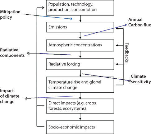
Figure 9.1 A policy that changes one of the above aspects changes all aspects and how they develop influence each other over time
As shown in this figure, the primary interest is to create policy guidelines that would mitigate impact of emissions, primarily the CO2.
Nordhaus is the developer of the DICE and RICE models3 integrated assessment models of the interplay between economics, energy use, and climate change. In his books on climate change he started off with the assumption that greenhouse gases are positively responsible for the climate change. From that point onward, he never checked the validity of that assumption despite numerous historical data available to him (Nordhaus, 2008).
As early as 1993, Nordhaus (1993) wrote:
“Mankind is playing dice with the natural environment through a multitude of interventions – injecting into the atmosphere trace gases like the greenhouse gases or ozone-depleting chemicals, engineering massive land-use changes such as deforestation, depleting multitudes of species in their natural habitats even while creating transgenic ones in the laboratory, and accumulating sufficient nuclear weapons to destroy human civilizations” (p. 11).
In this paper, he puts greenhouse gases in the same line with ozone-depleting chemicals (that would be CFC). He attacks massive land-use changes, including deforestation and laments depletion of certain species in the process. He even criticizes genetic alterations as well as nuclear weapons. He makes no comment on pesticide, chemical fertilizer and more importantly the chemical industry that is in control of oil refining and gas processing. He also makes no comment about the possibility of greenhouse gases being natural, thus harmless to the ecosystem.
His projection umbers are shown in Figure 9.2. In this figure, projections of IPCC Report are (dashed lines) from Intergovernmental Panel on Climate Change (1990) and that with the DICE model, which was developed by Nordhaus. We have discussed the shortcomings of these models in Chapter 2, but what is important here is the claim that this projection has scientific merit, although it has practically no relevance to the real problem and has nill data that could be cited for fine tuning the models. Also, note this was a prediction some 25 years ago, during the time Al Gore was fully involved in creating the climate change hysteria.

Figure 9.2 Projection of global temperature change as per Nordhaus (1993).

Figure 9.3 Labour price of light (After Nordhaus, 1998).
In 1998, Nordhaus authored a seminal report, in which he argued technological progress has delivered astonishing changes in the availability of artificial light, from the sesame oil lamps used in Babylon in 2000 BCE, to the first gas lamps used in the 1790s, to the LEDs we use today. Without regard to the hidden cost of artificial light, he proceeded to compare progress with a staggering drop in the cost of light, as measured in the number of hours one would have to work to buy one lumen. With that argument, he showed a steep decline since the Industrial Revolution. In the Middle Ages, an average person might have had to work for 10 hr to afford a thousand lumen hours of light. By 2000, that was down to working for about a third of a second.
He also introduced the concept of ‘true price index’. He took the period of 1883 (when Edison first introduced electric light) to 1993 (time of publication) and lumped gas and kerosene lights together because they were about the same price in that era. Figure 9.4 Shows that the prices of the fuel rose by a factor of 10 for kerosene and by a factor of 3 for electricity. He argued that if an ideal traditional (frontier) price index were constructed, it would use late weights (following electricity prices) since it is the frontier technology. Hence, the ideal traditional (frontier) price index using the price of inputs would show a fall in the price of light by a factor of 3 over the last century. On the other hand, if the price index were incorrectly constructed, say by using 1883 consumption weights and tracking gas/kerosene prices, it would show a substantial upward increase by a factor of 10. A true (frontier) price index of output or illumination, according to Nordhaus, would track the lowest solid line (Figure 9.4), which shows a decline factor of 75 over the century of concern. In summary, it shows a much steeper decline in price relative to the price of electricity because of the improvements in the efficiency of electricity. How such an extra ordinary efficiency can appear? Chhetri and Islam (2008) pointed out that such a number can be concocted by including only one portion of the energy picture. Similar to what has been ubiquitous today in terms of high efficiency of electric or hybrid cars all because the background of the electricity is not included, assigning such high value amounts to selective bias in favour of electric energy. It is no small irony that Nordhaus calls the conventional procedure ‘biased’.
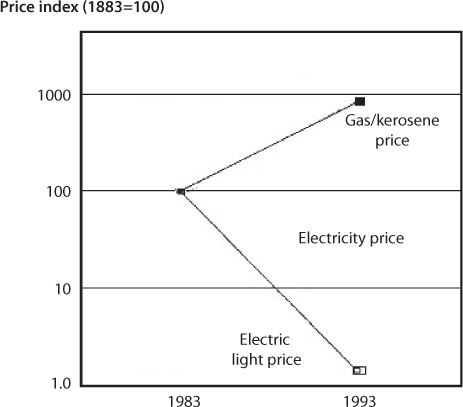
Figure 9.4 Energy pricing as seen by Nordhaus.
Nordhaus (1993) introduced his DICE model in the realm of science. However, the principal conclusion of this paper was that there should be a carbon tax. Without any scientific evidence, the paper started off with the conclusion that “a modest carbon tax would be an efficient approach to slow global warming, while rigid emissions-stabilization approaches would impose significant net economic costs.” This so-called ‘Dynamic Integrated Climate-Economy model’ claimed to have included dynamic policies as well as dynamic data. This was an improvement over past model that was steady state. Following assumptions were made:
- The economy is endowed with an initial stock of capital, labor, and technology, and all industries behave competitively;
- Each country maximizes an intertemporal objective function, identical in each region, which is the sum of discounted utilities of per capita consumption times population;
- Output is produced by a Cobb-Douglas production function in capital, labor, and technology;
- Population growth and technological change are exogenous, while capital accumulation is determined by optimizing the flow of consumption over time.
On the technological side, In modeling GHG emissions, Nordhaus assumes that the ratio of uncontrolled GHG emissions to gross output is a slowly moving parameter represented by σ(t). GHG emissions can be reduced through a wide range of policies is the fundamental assumption of his work. In this analysis, an ‘emissions control factor’, μ(t) is introduced so that the amount of CO2 can be reduced and its impact studied. This term is the fractional reduction of emissions relative to the uncontrolled level. Scientifically, this emission controlling factor has no meaning other than for a parametric study. It assumes that somehow emissions can be reduced and as a consequence, he wants to study what happens to the rest of climate. So, Nordhaus is merely looking at how to optimize the trajectory of emissions control. The emissions equation is given as:
Where, E(t) is GHG emissions, Q(t) is the gross output, σ(t) is determined from historical data, and it is assumed that GHG emissions were uncontrolled through 1990, meaning there was no reduction, µ(t), effectuated before that date. In addition to previous assumptions, this equation further assumes that Cobb–Douglas function of capital, labor, and technology applies to climate change. The most egregious aspect of this assumption is the conflation of anthropogenic CO2 with natural CO2 and application of mechanical relationship to nature, for which nothing of the modern engineering applies. Of course, the Cobb–Douglas production function was not developed on the basis of any knowledge of engineering, technology, or even management of the production process. It was instead developed because it had attractive mathematical characteristics, such as diminishing marginal returns to either factor of production and the property that expenditure on any given input is a constant fraction of total cost. Equation 9.1 serves as the basis for the entire DICE model and this represents the non-scientific nature of this model. Lindzen (2018) also called out the absurdity of using anthropogenic CO2 as the controlling parameter for global warming, although it represents miniscule portion of the global CO2 output.
The next part of the model introduces a number of relationships that attempt to capture the major forces affecting climate change. It is assumed that there is instant mixing of various gases. The following equation is assumed to govern the CO2 accumulation.
where M(t) is the change in concentrations from pre-industrial times, β is the marginal atmospheric retention ratio, and δM is the rate of transfer from the quickly mixing reservoirs to the deep ocean. Similar to Eq. 9.1, Eq. 9.2 is the GHG analog of the capital accumulation equation. Atmospheric concentrations in a period are determined by last period’s concentrations [M(t- l)] times (l-δM,), where δM is the rate of removal of GHGs. This approximation essentially assumes that none of the CO2 emitted is absorbable within the ecosystem. With this formulation, another series of linear relationship between CO2 accumulation and climate change are invoked. The climate system is represented by a multilayer system, namely three layers - the atmosphere, the mixed layer of the oceans, and the deep oceans - each of which is assumed to be well mixed. This is the crudest version of the 2-layer atmospheric model, as discussed in Chapter 2. It also assumes instant mixing and adiabatic wall – both illogical in a natural setting. The accumulation of GHGs is assumed to warm the atmospheric layer, which then warms the mixed ocean, which in turn diffuses into the deep oceans. The lags in the system are primarily due to the thermal inertia of the three layers. This model is written as:
(9.3)

where T(t)=temperature of layer i in period t (relative to the pre-industrial period); i = 1 for the atmosphere and upper oceans (rapidly mixed layer) and i = 2 for the deep oceans; F(t)=radiative forcing in the atmosphere (relative to the pre-industrial period); Ri = the thermal capacity of the different layers; τ2 = the transfer rate from the upper layer to the lower layer; and λ=the transfer rate f
The above expression essentially treats the atmosphere like a laboratory flask and presumes that the data available to calibrate the model are as abundantly available as a laboratory test.
Ignoring the fact that the above formulation has no scientific basis, Nordhaus proclaims that the most important shortcoming is that the damage function, particularly the response of developing countries and natural ecosystems to climate change, is poorly understood at present. This apparent admission of shortcoming diverts attention to the fact that the formulation has no scientific basis and the fundamental assumptions involved are fatally flawed and illogical. What it does in addition is to create hysteria. Note the following disclaimer:
“… the potential for catastrophic climatic change, for which precise mechanisms and probabilities have not been determined, cannot currently be ruled out. Furthermore, the calculations omit other potential market failures, such as ozone depletion, air pollution, and R&D, which might reinforce the logic behind greenhouse gas reduction or carbon taxes. Issues of sensitivity analysis with respect to either parameters or components of the model have not been addressed in this study, although an examination of these issues is underway, as discussed above. And finally, this study abstracts from issues of uncertainty, in which risk aversion and the possibility of learning may modify the stringency and timing of control strategies.”
However, this formulation would set the stage for universal carbon tax decades later. To the credit of Nordhaus, other scientists have been duped into taking his conclusions as facts and the entire debate has been surrounding peripheral issues, without focus on the core lack of science in DICE formulation (see for instance, Kelly and Kolstad, 2001). Economists served as the drum beater of the climate change proponents. Consider the following quote of Fatih Birol, executive director of the International Energy Agency, explains his warning that oil prices may be entering the “red zone”.
“It seems like expensive energy is back, and back at the wrong time for the global economy … Global economic growth is losing momentum, there are major currency issues in emerging countries, and trade tensions among major players” (Quoted by Financial Times, 2018).
Subsequent versions of DICE have been used by policymakers to investigate alternative approaches to slowing climate change, namely through the application of carbon taxes. This line of cognition dominates Nordhaus’ take on ‘economics of climate change’. He was not challenged and he continued to make his mark on energy politics. He co-edited an NRC report that concluded that the current federal tax provisions have minimal net effect on greenhouse gas emissions, according to a new report from the National Research Council. The report found that several existing tax subsidies have unexpected effects, and others yield little reduction in greenhouse gas emissions per dollar of revenue loss. This report was a result of Congressional request to evaluate the most important tax provisions that affect carbon dioxide and other greenhouse gas emissions and to estimate the magnitude of the effects. The report considered both energy-related provisions – such as transportation fuel taxes, oil and gas depletion allowances, subsidies for ethanol, and tax credits for renewable energy – as well as broad-based provisions that may have indirect effects on emissions, such as those for employer-provided health insurance, owner-occupied housing, and incentives for investment in machinery.
Using energy economic models based on the 2011 U.S. tax code, the committee found that the combined effect of energy-related tax subsidies on greenhouse gas emissions is minimal and could be negative or positive. It noted that estimating the precise impact of the provisions is difficult because of the complexities of the tax code and regulatory environment. However, it found that these provisions achieve very little greenhouse gas reductions at substantial cost; the U.S. Department of the Treasury estimates that the combined federal revenue losses from energy-sector tax subsidies in 2011 and 2012 totalled $48 billion. The report concluded that while few of these provisions were created solely to reduce greenhouse gas emissions, they are a poor tool for doing so. In this process, no one questioned the source of the greenhouse gases that they were trying to reduce. As we will see in latter section of this chapter, greenhouse gases from manmade activities are miniscule compared to what is emitted naturally.
Not surprisingly, the models indicated that the provisions subsidizing renewable electricity reduce greenhouse gas emissions, while those for ethanol and other biofuels may have slightly increased greenhouse gas emissions. However, the debate delved into national output. They suggested that broad-based provisions such as tax incentives to increase investment in machinery affect emissions primarily through their effect on national economic output. In other words, when a broad-based tax provision is removed, the percent change in emissions is likely to be close to the percent change in national output.
It was quite stunning that the committee came up with the recommendation that tax provisions and climate change policy can make a substantial contribution to meeting the nation’s climate change objectives, although they themselves determined that the current approaches were ineffective in making any dent on the greenhouse gas emission. Without any evidence, and in fact with evidence to the contrary, they recommended that carbon taxes or tradable emissions allowances, would be the most effective and efficient ways of reducing greenhouse gases. Their science had no logic and there was a total disconnection between what was observed and what was recommended.
Ever since the development of DICE and RICE models, no science has been added to those strictly empirical model, yet they have been assigned the name ‘science-based’ and the entire debate has been over how much emission reduction must be imposed and what carbon tax must be levied.
Then came the presentation of Nobel Prize in Economic sciences and the latest model, DICE-2016R2 was instantly sanctified and its predictions under presents four different scenarios, each applying a different carbon tax amount were gilded as the epitome of science-based policy making. The Nobel Committee tweeted,
“Laureate William Nordhaus’ research shows that the most efficient remedy for problems caused by greenhouse gas emissions is a global scheme of carbon taxes uniformly imposed on all countries. The diagram shows CO2 emissions for four climate policies according to his simulations.”
The Base case involves no new climate change policy beyond 2015 policies. The Opt option involves carbon taxes that maximize global welfare, using conventional economc assumptions about the importance of the welfare of future generations. The Stern option involves carbon taxes that maximize global welfare, with substantially more emphasis on the welfare of future generations than in scenario two as suggested in the Economics of Climate Change: The Stern Review, from 2007. The T < 2.5 option involves carbon taxes high enough to keep global warming from ever exceeding 2.5 C are implemented at minimum global welfare cost. If one had any doubt this is the epitome of knowledge, the following picture was plastered as a reminder, civilization has arrived and we are about to embark on the ultimate enlightenment, as depicted in Picture 9.1.

Picture 9.1 New Science has introduced a version of science that includes fundamental false assumptions that are in line with the desired outcome.
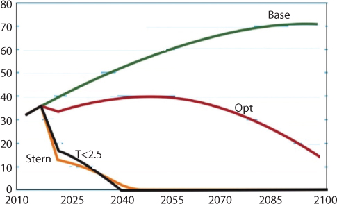
Figure 9.5 Predicted CO2 emissions tweeted by the The Royal Swedish Academy of Sciences (credit to Johan Jarnestad/The Royal Swedish Academy of Sciences, 2018).
What we have here is a correlation and a discussion around that correlation without first establishing or even stating the theory. Of course, correlation doesn’t mean causation, so science doesn’t accept everything that correlates. Before correlation comes the link to causation. Repeatedly scientists have fallen into this ‘correlation means causation’ argument. Yet, the science used has been analogous to the pirate vs. global warming correlation (Figure 9.6). This figure available on Internet and previously used by Islam et al. (2010a) to show the spurious nature of modern-day probability theories presents a case, in which an absurd correlation between number of pirates with natural disasters is sought. The conclusion derived from this plotting is that global warming, earthquakes, hurricanes, and other natural disasters are a direct effect of the shrinking numbers of Pirates since the 1800s. At this point, the debate becomes how accurate the correlation is and what can be done to bring up the number of pirates without invoking too much disturbance in the high sea. This metaphor helps understand the problem associated with modern day connection between global warming, CO2 concentration and carbon tax.

Figure 9.6 Illustration of how an absurd conclusion cannot be avoided unless true science is introduced.
Without any scientific basis, the decades old empirical model now has assumed the place of the most scientifically accurate predictive tool and forecasts are exact and final. For instance, if carbon taxes were 6 to 8 times higher than today’s levels, drastic emission cuts could be achieved over a 25 year period (and maintained for much longer). The one-sided research shows how economic activity and policymaking (the creation and application of taxes) can interact with basic chemistry and physics (the carbon emissions) to slow climate change. For example, if the highest level taxes were applied, global warming temperatures could be kept from exceeding 2.5 C. Note the value 2.5 how closely it hovers around the almost century old 3 C that was picked out of thin air and flaunted as the ultimate number for climate change.
Yet, anytime this ‘science’ is challenged, insults are dolled out. Within minutes of Nobel Committee flaunting carbon tax as the only solution to save humanity, the following insulting tweets were directed toward a tweet that attempted to talk logic (Screenshort 9.1).
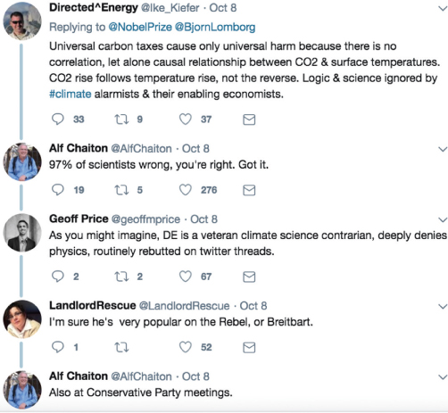
Screenshort 9.1 Twitter feeds in response to the announcement of Universal carbon tax.
9.3 Historical Development
Progress in humanity is synonymous with how we manage our energy needs. Notwithstanding what is routinely put out in popular science and mainstream media, the energy crisis that we face today is not a result of continuous progress in society, let alone the product of human evolutionary traits. The current civilization is unique in the sense that no other epoch has been fixated on fear and greed the way this current world has been. In today’s culture of fear and greed, in which every fear is perpetrated in order to scheme off the scared population, there are many tactics that are in place. The most popular one is that we are in every war because it is about oil. Then, the scientific community, which is also another sellout to the grand scheme, rings another warning bell, we are soon to run out of oil, and there must be another resource put in place for an extra cost. The moment we make progress toward increasing the oil supply through new techniques of oil extraction, expansion of resource base, there comes another debilitating fear – the global warming. It used to be the so-called peak oil theories that popped out from all corners. It is the same hype that was concocted in last century about the world running out of coal. Then comes another round of apoplectic messiahs that warn us about global warming and vilifying carbon – of all things – as the enemy of life on earth. Before anyone can get out of gasping, the economists come out and ring another warning bell – all these have to be remedied for a fee and we simply do not have enough to go around.
In this section, the history of technological development from the pre-industrial age to the petroleum is reviewed. There is a colloquial expression to the effect that exact change plus faith in the Almighty will always get you downtown on the public transit service. On the one hand, with or without faith, all kinds of things could happen with the public transit service, before the matter of exact fare even enters the picture. On the other hand, with or without exact fare, other developments could intervene to alter the availability of the service and even cancel it. This helps isolate one of the key difficulties in uncovering and elaborating the actual science of increased carbon-dioxide concentrations in the atmosphere. All kinds of activities can increase CO2 output into the atmosphere; but precisely which activities can be held responsible for consequent global warming or other deleterious impacts? Both the activity and its CO2 output are necessary, but neither by itself is sufficient, for establishing what the impact may be and whether it is deleterious. The delinearized history has to involve different epochs divided up by pre- and post-industrial age and then the petroleum era. Of course, the CO2 emission history uses pre-industrial period as the benchmark. However, when it comes to causation, petroleum industry is held accountable for the rise in CO2 level. Therefore, we have to study the petroleum period separately.
9.3.1 Pre-Industrial
One commonly encountered argument attempts to frame the historical dimension of the problem, more or less, as follows: once upon a time, the scale of humanity’s efforts at securing a livelihood was insufficient to affect overall atmospheric levels of CO2. The implication is that, with the passage of time and the development of more extensive technological intervention in the natural-physical environment, everything just got worse. However, from prehistoric times onward, there have been important periods of climate change in which the causes could not have had anything to do with human intervention in the environment, especially not at the level we see today that is widely blamed for “global warming.”
Nevertheless, these had consequences that were extremely significant and even devastating for wide swaths of subsequent human life on this planet. One of the best-known climate changes was the period of almost two centuries of cooling in the northern hemisphere during the 13th and 14th centuries CE, in which Greenland is said to have acquired much of its most recent ice cover. This definitively brought to an end any further attempts at colonizing the north and northwest Atlantic by Scandinavian tribes (descended from the Vikings), creating the opening for later commercial fisheries to expand into the northwest Atlantic by using Basque, Spanish, Portuguese and eventually French and British fishermen and fishing enterprises – the starting-point of European colonization of the North American continent.
9.3.2 Industrial Age
The Industrial Age will be remembered as the epoch that founded the culture of Dogma justified with the hubris of science. The critical review of all major theories (scientific as well as social) demonstrates that the most fundamental and fatal shortcoming of these theories is their fundamental premises that are spurious or unnatural (Islam et al., 2018a). In fact, every diagnosis process starts off with a spurious first premise, making the entire process aphenomenal. Not surprisingly, every publication comes up with a different explanation for the same set of data. The problem is further convoluted by the fact there is no standard theory that is free from inherent spurious premises (Islam et al., 2014). Yet, there is no shortage of hubris from both scientists and social scientists. Wilhelm Ostwald (1853–1932, recipient of the 1909 Nobel Prize in Chemistry for his work on catalysis) was credited for expanding explicitly “the second law of energetics to all and any action and in particular to the totality of human actions…. All energies are not ready for this transformation, only certain forms which have been therefore given the name of the free energies…. Free energy is therefore the capital consumed by all creatures of all kinds and by its conversion everything is done” (Ostward, 1912; quoted by Smil, 2017). Ostwald is usually credited with inventing the Ostwald process (patent 1902), used in the manufacture of nitric acid, although the basic chemistry had been patented some 64 years earlier by Kuhlmann. The science that Ostward introduced would pave the way to developing chemical fertilizers that triggered ‘green revolution’ around the world in 1960s. This ‘revolution’ was completed with another ‘miraculous’ technology in name of DDT, which fetched a Nobel prize for Paul Hermann Müller in 1948, only to be banned in 1972. We have seen in previous chapter how consequential these technological breakthroughs have been to the environment, in particular to the carbon culture.
It is the same story in social science and economics. The term “social science” first appeared in the 1824 book An Inquiry into the Principles of the Distribution of Wealth Most Conducive to Human Happiness. This ‘happiness’ applied to the Newly Proposed System of Voluntary Equality of Wealth by William Thompson (1775–1833). The concern for social equality was in the core of the social thinking but did not have a definite form, let alone concrete theories. Auguste Comte (1797–1857) argued that ideas pass through three rising stages, theological, philosophical and scientific. He defined the difference as the first being rooted in assumption, the second in critical thinking, and the third in positive observation. This framework, still rejected by many, encapsulates the thinking which was to push economic study from being a descriptive to a mathematically based discipline. Karl Marx was one of the first writers to claim that his methods of research represented a scientific view of history in this model. With the late 19th century, attempts to apply equations to statements about human behavior became increasingly common. Among the first were the “Laws” of philology, which attempted to map the change over time of sounds
After Newton, all modern European social theories are premised on considering humans as ‘just another species’, disconnecting human conscience or consciousness from human behavior. Malthus (1766–1834), who inspired the likes of Charles Darwin, Paul R. Ehrlich, Francis Place, Raynold Kaufgetz, Garrett Hardin, John Maynard Keynes, Pierre François Verhulst, Alfred Russel Wallace, William Thompson, Karl Marx, Mao Zedong, introduced this false premise.
Blumer (1954) dared question social theories advanced in the enlightened world, albeit limited to empirical science. He wrote:
“Now, it should be evident that concepts in social theory are distressingly vague. Representative terms like mores, social institutions, attitudes, social class, value, cultural norm, personality, reference group, social structure, primary group, social process, social system, urbanization, accommodation, differential discrimination and social control do not discriminate cleanly their empirical instances. At best they allow only rough identification, and in what is so roughly identified they do not permit a determination of what is covered by the concept and what is not.”
All modern European social theories are premised on considering humans as ‘just another species’, disconnecting human conscience or consciousness from human behavior (Islam et al., 2013). Here, we will discuss one of the most widely accepted (consciously or otherwise) theories that is based on the premise that humans are liabilities. This theory is in the core of all other theories, including peak oil theory. Reverend Thomas Robert Malthus, a British scholar advanced the theory of rent. In his publications during 1798 through 1826, he identified various factors that would affect human population. For him, the population gets controlled by disease or famine. His predecessors believed that human civilization can be improved without limitations. Malthus, on the other hand thought that the “dangers of population growth is indefinitely greater than the power in the earth to produce subsistence for man”. He added his religious fervor to this doctrine and considered it divine and wrote:
“Must it not be acknowledged by an alternative examiner of the histories of mankind, that in every age and in every State in which man has existed, or does now exist that the increase of population is necessarily limited by the means of subsistence, that population does invariably increase when the means of subsistence increase, and, that the superior power of population is repressed, and the actual population kept equal to the means of subsistence, by misery and vice.”
He supported the Corn Laws and opposed the poor law. The poor law had been in place for centuries to deal with the ‘nuisance’ of beggars and ‘impotent poor’. The Corn Laws were supposed to protect local farmers from less expensive imports of wheat and other food grains. The Corn Laws needs a bit elaboration. In 1816, the volcanic eruption in the Indonesian archipelago incurred tremendous consequences. It spewed an enormous volume of dust into the atmosphere that travelled around the globe in the jet stream and led to the “year with no summer” in Europe and the northern half of North America. In 1817, grain crops on the continent of Europe failed. In industrial Great Britain, where the factory owners and their politicians boasted how the country’s relatively (compared to the rest of the world) highly advanced industrial economy had overcome the “capriciousness of Nature,” hunger and famine actually stalked the English countryside for the first time in more than a century and a half. The famine conditions were blamed on the difficulties attending the import of extra supplies of food from the European continent and led directly to a tremendous and unprecedented pressure to eliminate the Corn Laws – the system of high tariffs protecting English farmers and landlords from the competition of cheaper foodstuffs from Europe or the Americas. Politically, the industry lobby condemned the Corn Laws as the main obstacle to cheap food, winning broad public sympathy and support. Economically, the Corn Laws actually operated to keep hundreds of thousands employed in the countryside on thousands of small agricultural plots, at a time when the demands of expanding industry required uprooting and forced the rural population to work as factory laborers. Increasing the industrial reserve army would enable British industry to reduce wages. Capturing command of that new source of cheaper labor was, in fact, the industrialists’ underlying aim.
Without the famine of “the year with no summer,” it seems unlikely that British industry would have targeted the Corn Laws for elimination, therefore blasting its way into dominating world markets. Even then, because of the still prominent involvement of the anti-industrial lobby of aristocratic landlords who dominated the House of Lords, it would take British industry nearly another 30 years. Between 1846 and 1848 Parliament eliminated the Corn Laws, industry captured access to a desperate workforce fleeing the ruin brought to the countryside, and overall industrial wages were driven sharply downwards. On this train of economic development, the greatly increased profitability of British industry took the form of a vastly whetted appetite for new markets at home and abroad, including the export of important industrial infrastructure investments in “British North America,” i.e., Canada, Latin America, and India. Extracting minerals and other valuable raw materials for processing into new commodities in this manner brought an unpredictable level of further acceleration to the industrialization of the globe in regions where industrial capital had not accumulated significantly, either because traditional development blocked its role or because European settlement remained sparse.
Malthus’ theories were later rejected based on empirical observations that confirmed that famine and natural disasters are not the primary cause of population control. Many economists, including, Nobel Laureate Economist Amartya Sen (1998) who confirmed the man-made factor playing a greater role in controlling the human population. However, Malthus’ theory lives on in every aspect of European social science and hard science. Malthus’ most notable follower was Charles Darwin whose theory of natural selection is eerily similar to Mathusian theory. They are similar in two ways: 1) they both assume that humans are just another species, thus disconnecting human conscience from human being; 2) they both use natural causes as the sole factor in deciding human population, thus inferring they knew the underlying program of nature science. Of more significance is the fact that Darwin was considered to be a ‘hard scientist’ whereas Malthus was considered to be a social scientist and an economist. This aspect needs some elaboration. Darwin said that the emergence of a species distinct in definite ways from its immediate predecessor and new to the surrounding natural environment generally marked the final change in the sequence of steps in an evolutionary process. The essence of his argument concerned the non-linearity of the final step, the leap from what was formerly one species to distinctly another species. Darwin was silent on the length of time that may have passed between the last observed change in a species-line and the point in time at which its immediate predecessor emerged – the characteristic time of the predecessor species – was the time period in which all the changes so significant for later on were prepared. This latter could be eons, spanning perhaps several geological eras. This idea of tNATURAL as characteristic time is missing from every European theorist. This is not unexpected. Ever since the work of Thomas Aquinas, Europeans scientists simply repeated the dogmatic adherence to tangible timelines while distancing themselves from doctrinal philosophy. However, as Islam et al. (2018a) have recently pointed out, they did not employ the scientific methodology of Averroes while accepted him as the father of secular philosophy in Europe as well as claimed themselves to be secular. This claim was not genuine. A second, but equally telling source of pressure on social scientists to mathematize their research methodology was a sense that their work would not be taken seriously as scientific without some such mathematical rigor. As the models and mathematics from the so-called “exact” sciences would hardly be appropriate or seem credible in any field of study focusing on human beings and their incredible variety of needs, wants and impulses, another kind of mathematics would have to do. This fascination comes from another trail of cognition that was popularized when the term social science was introduced. Questions of history and historical phenomena were also a convenient target because of the lack of any means to describe them with any meaningful, non-trivial mathematical model.
In terms of economics and purely social theory, John Maynard Lord Keynes was probably the biggest supporter of Malthus. Similar to Malthus, Keynes also believed that historical time had nothing to do with establishing the truth or falsehood of economic doctrine. “In the long run, we are all dead,” he wrote. He tied this to a stance that attacked all easy acceptance without question of any of the underlying assumptions propping up all forms of orthodoxy. Accordingly, this retort was taken as the sign of a fresh and rebellious spirit. However, in his own theoretical work he was frequently at pains to differentiate what happens to individuals who are driven by short-term considerations from what happens at the societal level at which he was theorising about broad historically sweeping movements of economic cause and effect (Keynes, 1936).
Keynes would emerge completely unscathed. No one challenged his theories that were accepted at face value with doctrinal fervor. Until now, every Nobel Laureate in Economics derives his/her inspiration from Keynes. One of them is Stiglitz, who was deconstructed by Zatzman and Islam (2007) as well as Zatzman (2012, 2013).
Even though not explicitly recognized for obvious reasons, Karl Marx also derived his inspiration from Malthus and did little to change the premise that Malthus built his theories on. For Karl Marx, however, human beings did have connection to the conscience but that conscience was solely dedicated to “survival”. This ‘conscience’ is not any different from what has been known as ‘instinct’ – something that every animal has. This survival, in Marx’s belief, was the reason for dialectic materialism and class struggle. Similar to what has been pointed out in the discourse on human civilization (Islam et al., 2013, 2014a, 2014b, 2014c), the only possibility that Karl Marx did not investigate is the existence of higher conscience that makes a human unselfish and considerate of long-term consequence. Such deviation from long-term approach is strictly Eurocentric. Such addiction to short-term approach was non-existent prior to Thomas Aquinas and the adoption of doctrinal philosophy.
What made Karl Marx popular is his empathy for the poor and the oppressed. His notion of capitalism being the “dictatorship of bourgeoisie”, a notion by itself is based on the same premise of ‘human being is an evil animal’ that Karl Marx used, hit a sympathetic cord with a wide range of followers. Similar to what Malthus predicted in terms of population control by famine and natural disasters, Karl Marx predicted that Capitalism would be subject to internal conflicts and will implode, being replaced with socialism. This in turn will lead to the replacement of “dictatorship of bourgeoisie” with “dictatorship of proletariat”. His theory was so convincing that Soviet Union was formed in 1922, leading the way to many countries that formally adopted Marxism as the formal political system of the country. In 1949, the People’s Republic of China became communist, making nearly half of the world population to immerse into a political system that can be best described as the dream application of Karl Marx’s political theory. Marx is recognized as one of the most influential person of all time (Hart, 2000). Yet, the prediction of Karl Marx that capitalism will be replaced with socialism and eventually give rise to stateless, classless society has utterly failed. Instead of stateless society ruled by “workers”, socialism created the biggest and most repressive government regimes of human history. Many celebrate the fact that every promise of capitalism has made in terms free market economy has been broken and monopoly has become the modus operandi of biggest corporations of ‘free market’ economy, but few point out that such is the demise of Marxist predictions in societies that did everything to uphold Marx’s ideals.
Even events like the volcanic eruption in the Indonesian archipelago in 1816 incurred tremendous consequences. It spewed an enormous volume of dust into the atmosphere that travelled around the globe in the jet stream and led to the “year with no summer” in Europe and the northern half of North America. In 1817, grain crops on the continent of Europe failed. In industrial Great Britain, where the factory owners and their politicians boasted how the country’s relatively (compared to the rest of the world) highly advanced industrial economy had overcome the “capriciousness of Nature,” hunger and famine actually stalked the English countryside for the first time in more than a century and a half. The famine conditions were blamed on the difficulties attending the import of extra supplies of food from the European continent and led directly to a tremendous and unprecedented pressure to eliminate the Corn Laws – the system of high tariffs protecting English farmers and landlords from the competition of cheaper foodstuffs from Europe or the Americas. Politically, the industry lobby condemned the Corn Laws as the main obstacle to cheap food, winning broad public sympathy and support. Economically, the Corn Laws actually operated to keep hundreds of thousands employed in the countryside on thousands of small agricultural plots, at a time when the demands of expanding industry required uprooting and forced the rural population to work as factory laborers. Increasing the industrial reserve army would enable British industry to reduce wages. Capturing command of that new source of cheaper labor was, in fact, the industrialists’ underlying aim. Without the famine of “the year with no summer,” it seems unlikely that British industry would have targeted the Corn Laws for elimination, therefore blasting its way into dominating world markets. Even then, because of the still prominent involvement of the anti-industrial lobby of aristocratic landlords who dominated the House of Lords, it would take British industry nearly another 30 years. Between 1846 and 1848 Parliament eliminated the Corn Laws, industry captured access to a desperate workforce fleeing the ruin brought to the countryside, and overall industrial wages were driven sharply downwards. On this train of economic development, the greatly increased profitability of British industry took the form of a vastly whetted appetite for new markets at home and abroad, including the export of important industrial infrastructure investments in “British North America,” i.e., Canada, Latin America, and India. Extracting minerals and other valuable raw materials for processing into new commodities in this manner brought an unpredictable level of further acceleration to the industrialization of the globe in regions where industrial capital had not accumulated significantly, either because traditional development blocked its role or because European settlement remained sparse.
9.3.3 Age of Petroleum
The modern era of oil production and the ensuing age of petro-politics began on August 27, 1859, when Edwin L. Drake drilled the first successful oil well 69 feet deep near Titusville in northwestern Pennsylvania. Just five years earlier, the invention of the kerosene lamp had ignited intense demand for oil. By drilling an oil well, Drake had hoped to meet the growing demand for oil for lighting and industrial lubrication. Drake’s success inspired hundreds of small companies to explore for oil. In 1860, world oil production reached 500,000 barrels; by the 1870s production increased phenomenally to 20 million barrels annually. In 1879, the first oil well was drilled in California; and in 1887 an oil well was drilled, in Texas. But as production boomed, prices fell and oil industry profits declined. However, in 1882, John D. Rockefeller had devised a solution to the problem of competition in the oil fields: the Standard Oil Trust. This brought together many of the leading refiners in the United States by controlling crude oil refining, the Trust was able to control the price of oil.
The world economy entered the Age of Petroleum with the rise of an industrial-financial monopoly in one sector of production after another in both Europe and America before and after World War I. Corresponding to this has been the widest possible extension of chemical engineering – especially the chemistry of hydrocarbon combination, hydrocarbon catalysis, hydrocarbon manipulation and rebonding – on which the refining and processing of crude oil into fuel and myriad byproducts, such as plastics and other synthetic materials, crucially depend. As a result, there is no activity, be it production or consumption, in any society today that is tied to the production and distribution of such an output where adding to the CO2 burden in the atmosphere can be avoided or significantly mitigated. In these developments, carbon and CO2 are, in fact, vectors carrying many other toxic compounds and byproducts of these chemically engineered processes. Atmospheric absorption of carbon and CO2 from human activities or other natural non-industrial activities would normally be continuous. However, what occurs when hydrocarbon complexes combine with inorganic and other substances, which occurs nowhere in nature, is much less predictable, and – on the available evidence – not benign, either. From a certain standpoint, there is logic in attempting to estimate the effects of these other phenomena by taking carbon and CO2 levels as vectors. However, there has never been any justification to assume the CO2 level itself is the malign element. Such a notion is a non-starter in science in any event, which raises the question: Just what is the role of science? Today, there is no large petrochemical company or syndicate that has not funded a study or group interested in CO2 levels as a global warming index – whether to discredit or to affirm such a connection. It is difficult to avoid the obvious inference that these very large enterprises, fiercely competing to retain their market shares against rivals, do not have a significant stake in engineering a large and permanent split in public opinion based on confusing their intoxication of the atmosphere with rising CO2 levels. Whether the consideration is refining for automobile fuels, processing synthetic plastics, or concocting synthetic crude, behind a great deal of the propaganda regarding “global warming” stands a huge battle among oligopolies, cartels, and monopolies over market share. The science of “global warming” is the only means that can separate the key question, “What is necessary to produce goods and services that are nature-friendly?” from the toxification of the environment as a byproduct of the anti-nature bias of chemical engineering in the clutches of the oil barons.
Up until the commencement of World War I in 1914, the United States produced between 60 and 70 percent of the worldwide oil supply. By 1920, oil production reached 450 million barrels – prompting fear that the United States was about to deplete the available reserves and, hence, run out of oil. In fact, Government officials predicted that oil reserves in the United States would last only ten more years. As fears grew that the oil reserves of the United States were seriously depleted, the search for oil turned to a worldwide basis. As a result, crude oil was discovered in Mexico at the beginning of the 20th Century, in Iran in 1908, in Venezuela during World War I, and in Iraq in 1927. Because of the politics of the time and the still-existing empires and/or colonies, many of the new discoveries occurred in areas dominated by Britain and the Netherlands: such as in the Dutch East Indies (now, Indonesia), Iran, and various British mandates in the Middle East. By 1919, Britain controlled 50% v/v of the proven world reserves of crude oil.
However, after World War I, a struggle for the control of world oil reserves erupted. The British, Dutch, and French excluded companies based in and originating in the United States from owning oil fields in territories under their sphere of control. Not surprisingly, the Congress of the United States retaliated in 1920 by adopting the Mineral Leasing Act, which denied access to American oil reserves to any foreign country that restricted American access to its reserves. The dispute was ultimately resolved during the 1920 s when American-based and owned oil companies were finally allowed to drill in the then British Middle East and also in the Dutch East Indies.
The fear that oil reserves in the United States were depleted to the point of near exhaustion ended abruptly in 1924, with the discovery of extensive crude oil fields in Texas, Oklahoma, and California. These discoveries, along with production of crude oil from fields in Mexico, the Soviet Union, and Venezuela, combined to significantly lower the price of crude oil. By 1931, with crude oil selling for 10 cents a barrel (which may be compared to a value – approximately $1.54 per barrel – much less than the current variable price of 50$ to $100 per barrel of oil), domestic oil producers in the United States demanded restrictions on production in order to raise prices. In fact, the major producers of crude oil – Texas and Oklahoma – passed state laws and stationed militia units at oil fields to prevent to enforce these laws and prevent drillers from exceeding production quotas. However, despite these measures, the price of crude oil continued to fall. In a final bid to solve the problem of overproduction, the federal government – under the National Recovery Administration (NRA) – imposed production restraints, import restrictions, and price control. After the Supreme Court of the United States declared the actions of the National Recovery Administration (i.e., the Federal government) to be unconstitutional, the Federal government took and additional step and imposed a tariff on foreign oil. During World War II, the oil surpluses of the 1930 s quickly disappeared – six billion barrels (6 × 10⁹ bbls) of the seven billion barrels (7 × 10⁹ bbls) of petroleum used by the allies during the war came from the United States. Again, there was concern that the United States was running out of oil.
On the other hand, world oil prices were at such low levels that in 1960 Iran, Venezuela, and oil producers in the Middle Eastern countries form an alliance (often referred to as a cartel) that became known as the Organization of Petroleum Exporting Countries (OPEC) to negotiate oil prices – for the most part, higher prices of crude oil. This price-fixing came to a head in the early 1970 s when the United States, which depended on the Middle East for a third of its oil, realized that foreign (non-domestic) oil producers were in a position to control and raise oil prices. The oil embargo of 1973 and 1974, during which oil prices quadrupled, and the oil crisis of 1978 and 1979, when oil prices doubled and emphasized the vulnerability of the United States to foreign producers (Yergin, 1991; Speight, 2011b; Yergin, 2011). However, the oil crises of the 1970 s had an unanticipated side-effect when higher oil prices stimulated conservation and exploration for new oil sources. As a result of increasing supplies and declining demand, oil prices fell from $35 a barrel in 1981 to $9 a barrel in 1986. The sharp slide in world oil prices was one of the factors that led Iraq to invade neighboring Kuwait in 1990 in a bid to gain control over a substantial portion (in excess of 40% v/v) of Middle Eastern oil reserves. On the other hand, there were oil-producing countries that existed and operated outside of the OPEC cartel which were responsible for producing 60% v/v of the world’s oil but they faced increasing production hurdles. Many of these non-OPEC producers had older, less productive wells and rising costs for new projects, and in some cases rising domestic demand, cut into the export totals, leading to increases in unconventional oil production (NPC, 2007).
Five of the world’s fifteen largest oil producers are outside of OPEC – those countries are Russia, the United States, China, Mexico, Canada, Norway, and Brazil. Some major producers, such as the United States, Mexico, and Norway, have experienced a decline in production in recent years but, on the other hand, non-OPEC production, although declining, has been bolstered by the significant increases in production from Brazil, Canada, Russia, and other former Soviet states (BP, 2008) as well as hitherto unavailable oil production from tight formations and from shale formations through expansion of hydraulic fracturing projects (Speight, 2015).
9.3.3.1 High-Acid Crude Oils and Opportunity Crudes
Within the petroleum family are two different types of crude oils based on price: (1) opportunity crude oils and (2) high acid crude oils. Opportunity crude oils are often dirty and need cleaning before refining by removal of undesirable constituents such as high-sulfur, high-nitrogen, and high-aromatics (such as polynuclear aromatic) components. A controlled visbreaking treatment would clean up such crude oils by removing these undesirable constituents (which, if not removed, would cause problems further down the refinery sequence) as coke or sediment. There is also the need for a refinery to be configured to accommodate opportunity crude oils and/or high acid crude oils which, for many purposes are often included with heavy feedstocks.
High acid crude oils are crude oil that contains considerable proportions of naphthenic acids which, as commonly used in the petroleum industry, refers collectively to all of the organic acids present in the crude oil (Shalaby, 2005: Rikka, 2007). By the original definition, a naphthenic acid is a monobasic carboxyl group attached to a saturated cycloaliphatic structure. However, it has been a convention accepted in the oil industry that all organic acids in crude oil are called naphthenic acids. Naphthenic acids in crude oils are now known to be mixtures of low to high molecular weight acids and the naphthenic acid fraction also contains other acidic species.
Naphthenic acids can be very water-soluble to oil-soluble depending on their molecular weight, process temperatures, salinity of waters, and fluid pressures. In the water phase, naphthenic acids can cause stable reverse emulsions (oil droplets in a continuous water phase). In the oil phase with residual water, these acids have the potential to react with a host of minerals, which are capable of neutralizing the acids. The main reaction product found in practice is the calcium naphthenate soap (the calcium salt of naphthenic acids). The total acid matrix is therefore complex and it is unlikely that a simple titration, such as the traditional methods for measurement of the total acid number, can give meaningful results to use in predictions of problems. An alternative way of defining the relative organic acid fraction of crude oils is therefore a real need in the oil industry, both upstream and downstream.
High acid crude oils cause corrosion in the refinery – corrosion is predominant at temperatures in excess of 180 °C (355°F) (Kane and Cayard, 2002; Ghoshal and Sainik, 2013) – and occurs particularly in the atmospheric distillation unit (the first point of entry of the high-acid crude oil) and also in the vacuum distillation units. In addition, overhead corrosion is caused by the mineral salts, magnesium, calcium and sodium chloride which are hydrolyzed to produce volatile hydrochloric acid, causing a highly corrosive condition in the overhead exchangers. Therefore these salts present a significant contamination in opportunity crude oils. Other contaminants in opportunity crude oils which are shown to accelerate the hydrolysis reactions are inorganic clays and organic acids.
In addition to taking preventative measure for the refinery to process these feedstocks without serious deleterious effects on the equipment, refiners will need to develop programs for detailed and immediate feedstock evaluation so that they can understand the qualities of a crude oil very quickly and it can be valued appropriately and management of the crude processing can be planned meticulously.
9.3.3.2 Oil From Tight Formations and From Shale Formations
In addition, oil from tight sandstone and from shale formations (tight oil) is another type of crude oil (Speight, 2014, 2015). Typically, tight oil is conventional oil that occurs in low-permeability reservoirs. The oil contained in such reservoirs will not flow to the wellbore without assistance from advanced drilling (such as horizontal drilling) and fracturing (hydraulic fracturing) techniques. There has been a tendency to refer to this oil as shale oil. This terminology is incorrect insofar as it is confusing and the use of such terminology should be discouraged as illogical since shale oil has been (for decades) the name given to the distillate produced from oil shale by thermal decomposition (Lee, 1990; Scouten; 1990; Speight, 2012, 2014, 2015).
Tight sandstone formations and shale formations are heterogeneous and vary widely over relatively short distances. Thus, even in a single horizontal drill hole, the amount recovered may vary, as may recovery within a field or even between adjacent wells. This makes evaluation of plays and decisions regarding the profitability of wells on a particular lease difficult. Production of oil from tight formations requires at least 15 to 20 percent natural gas in the reservoir pore space to drive the oil toward the borehole; tight reservoirs which contain only oil cannot be economically produced (EIA, 2013).
The challenges associated with the production of oil from shale formations are a function of their compositional complexities and the varied geological formations where they are found. These oils are light, but they are very waxy and reside in oil-wet formations. These properties create some of the main difficulties associated with oil extraction from the shale. Such problems include scale formation, salt deposition, paraffin wax deposits, destabilized asphaltene constituents, corrosion and bacteria growth. Multi-component chemical additives are added to the stimulation fluid to control these problems.
Oil from tight shale formation is characterized by low-asphaltene content, low-sulfur content and a significant molecular weight distribution of the paraffinic wax content. Paraffin carbon chains of C10 to C60 have been found, with some shale oils containing carbon chains up to C72. To control deposition and plugging in formations due to paraffins, the dispersants are commonly used. In upstream applications, these paraffin dispersants are applied as part of multifunctional additive packages where asphaltene stability and corrosion control are also addressed simultaneously.
Scale deposits of calcite, carbonates and silicates must be controlled during production or plugging problems arise. A wide range of scale additives is available. These additives can be highly effective when selected appropriately. Depending on the nature of the well and the operational conditions, a specific chemistry is recommended or blends of products are used to address scale deposition.
Another challenge encountered with oil from tight shale formations is the transportation infrastructure. Rapid distribution of shale oils to the refineries is necessary to maintain consistent plant throughput. Some pipelines are in use, and additional pipelines are being constructed to provide consistent supply. During the interim, barges and railcars are being used, along with a significant expansion in trucking to bring the various these oils to the refineries. Eagle Ford production is estimated to increase by a factor of 6: from 350,000 bpd to approximately 2,000,000 bpd by 2017. Thus, a more reliable infrastructure is needed to distribute this oil to multiple locations. Similar expansion in oil production is estimated for Bakken and other identified (and perhaps as yet unidentified) tight shale formations.
9.3.3.3 Natural Gas
The generic term natural gas applies to gas commonly associated with petroliferous (petroleum-producing, petroleum-containing) geologic formations. Natural gas generally contains high proportions of methane (a single carbon hydrocarbon compound, CH4) – higher molecular weight paraffins (CnH2n+2) generally containing up to eight carbon atoms may also be present in small quantities (Mokhatab et al., 2006; Speight, 2007, 2014). The hydrocarbon constituents of natural gas are combustible, but nonflammable non-hydrocarbon components such as carbon dioxide, nitrogen, and helium are also present in the minority and are regarded as contaminants.
In addition to the natural gas which exists in petroleum reservoirs, there are also those reservoirs in which natural gas may be the sole occupant. The principal constituent of natural gas is methane, but other hydrocarbons, such as ethane, propane, and butane, may also be present. Carbon dioxide is also a common constituent of natural gas as well as trace amounts of rare gases, such as helium, may also occur – certain natural gas reservoirs are a source of these rare gases. Just as petroleum varies in composition, natural gas also has varied composition depending upon the reservoir from which it is produced. Furthermore, differences in natural gas composition not only occurs between different reservoirs but wells in the same field may also produce natural gases that are different in composition (Speight, 1990, 2007; Mokhatab et al., 2006; Speight, 2014). Thus, there is no single composition of components which might be termed typical natural gas.
Like petroleum, natural gas has been known for many centuries, but its initial use was probably more for religious purposes rather than as a fuel. For example, gas wells were an important aspect of religious life in ancient Persia (modern-day Iran) because of the importance of fire in the religion of that region. In classical times these wells were often flared and must have been, to say the least, awe inspiring (Forbes, 1964). However, the use of petroleum has been relatively well documented (more so than natural gas) because of its use in warfare and as mastic for walls and roads (Henry, 1873; Abraham, 1945; Forbes, 1958a, 1958b, 1959; James and Thorpe, 1994).
There are several general definitions that have been applied to natural gas that require explanation. For example, associated or dissolved natural gas occurs either as free gas or as gas in solution in the petroleum. Gas that occurs as a solution in the petroleum is dissolved gas whereas the gas that exists in contact with the petroleum (gas cap) is associated gas. In addition, lean gas is gas in which methane is the major constituent and wet gas contains considerable amounts of the higher molecular weight hydrocarbons. Sour gas contains hydrogen sulfide whereas sweet gas contains very little, if any, hydrogen sulfide. In direct contrast to the terminology of the petroleum industry where the residue (residuum, resid) is the high boiling material left after distillation (Speight, 2014), residue gas is natural gas from which the higher molecular weight (higher boiling) hydrocarbons have been extracted and so is the lowest boiling hydrocarbon in natural gas. Finally casing head gas (casinghead gas) is derived from petroleum but is separated at the separation facility at the well-head.
To further define the terms dry and wet in quantitative measures, the term dry natural gas indicates that there is less than 0.1 gallon (one gallon, US,=264.2 m3) of gasoline vapor (higher molecular weight paraffins) per 1000 ft3 (one ft3 = 0.028 m3). The term wet natural gas indicates that there are such paraffins present in the gas, in fact more than 0.1 gal/1000 ft3.
Just as oil can be produced from tight shale formations (formations having less than 10% v/v porosity and less than 0.1 millidarcy permeability), natural gas is also produced from such formations. Such gas (also called shale gas) is a description for a field in which natural gas accumulation is locked in tiny bubble-like pockets within layered sedimentary rock such as shale and tight sandstone formations (Speight, 2015). Tight gas describes natural gas that is dispersed within low-porosity silt or sand areas that create a tight-fitting environment for the gas. In general, the same drilling and completion technology that is effective with shale gas can also be used to access and extract tight gas, even though the selection criteria for a given operation is dependent on many factors (Islam, 2014).
9.3.3.4 Heavy Oil
Heavy oil is a type of petroleum that is different from the conventional petroleum insofar as it is much more difficult to recover from the subsurface reservoir. This material (heavy oil) has a much higher viscosity (and lower API gravity) than conventional petroleum and recovery of heavy oil usually requires thermal stimulation of the reservoir (Speight, 2008, 2009, 2014).
Petroleum and heavy oil have been very generally, if not arbitrarily, defined in terms of physical properties – heavy oil was considered to be crude oil that had gravity somewhat less than 20° API with tar sand bitumen falling into the API gravity range <10°. For example, Cold Lake heavy crude oil has an API gravity equal to 12° and tar sand bitumen, usually has an API gravity in the range 5-10° (Athabasca bitumen = 8° API). However, classification of crude oil by the use of a single physical property is subject to the errors inherent in the analytical method (by which the property is determined) and must be used with caution (Speight, 2014).
However, while conventional crude oil is oil that flows naturally or that can be pumped without being heated or diluted, heavy crude oil usually requires thermal stimulation to cause recovery. In fact, a more appropriate definition of heavy oil is that it is it is recoverable in its natural state by conventional oil well production methods including currently used enhanced recovery techniques. By analogy, tar sand bitumen it is not recoverable in its natural state using enhanced (tertiary) recovery techniques (Speight, 2009, 2013c, 2014).
The term extra heavy oil has been introduced fairly recently (without any reasonable scientific or engineering justification) and has only served to confuse the issues of nomenclature. Realistically, the termcan be used to define the high-boiling bituminous material that occurs in the near-solid state but which is capable of free flow under reservoir conditions (Speight, 2009, 2013c, 2014).
9.3.3.5 Tar Sand Bitumen
Throughout this text, frequent reference is made to tar sand bitumen, which is the bituminous material that occurs in tar sand deposits and is immobile under deposit conditions. Commercial recovery of bitumen from tar sand deposits in Canada have been in place for over 40 years (Speight, 2014) and, thus, it is not surprising that more is known about the Alberta (Canada) tar sand reserves than any other reserves in the world.
By way of further explanation, the term bitumen (also, on occasion, incorrectly referred to as native asphalt, since asphalt is a refinery product) includes a wide variety of naturally-occurring brown to black materials of semisolid, viscous-to-brittle character that can exist in nature with no mineral impurity or with mineral matter content that exceeds 50% by weight. Bitumen is frequently found filling pores and crevices of sandstone, limestone, or argillaceous sediments, in which case the organic and associated mineral matrix is known as rock asphalt. Tar sand bitumen is a high-boiling material with little, if any, material boiling below 350 °C (660 °F) and from which synthetic crude oil is produced by thermal processes (Speight, 2013c, 2014). The term oil sand is also used in the same way as the term tar sand, and these terms are used interchangeably throughout this text.
It is incorrect to refer to bitumen as tar or pitch. Although the word tar is somewhat descriptive of the black bituminous material, it is best to avoid its use with respect to natural materials. More correctly, the name tar is usually applied to the heavy product remaining after the destructive distillation of coal or other organic matter. Pitch is the distillation residue of the various types of tar. Alternative names, such as bituminous sand or oil sand, are gradually finding usage, with the former name (bituminous sands) more technically correct.
For the purposes of this text, the definition of tar sand bitumen is derived from the definition of tar sand that has been defined by the United States government (FE-76–4):
“[Tar sands] … the several rock types that contain an extremely viscous hydrocarbon which is not recoverable in its natural state by conventional oil well production methods including currently used enhanced recovery techniques. The hydrocarbon-bearing rocks are variously known as bitumen-rocks oil, impregnated rocks, oil sands, and rock asphalt.”
By inference, heavy oil is that resource which can be recovered in its natural state by conventional oil well production methods including currently used enhanced recovery techniques. The term natural state means without conversion of the heavy oil or bitumen as might occur during thermal recovery processes (Speight, 2009, 2014).
Nevertheless, whatever numbers are used, bitumen in tar sand deposits represents a potentially large supply of usable energy (Speight and Islam, 2016), in spite of the negatives comments that continue to be used about the resource (Levant, 2010). However, many of these reserves are only available with some difficulty and optional refinery scenarios will be necessary for conversion of these materials to low-sulfur liquid products because of the substantial differences in character between conventional petroleum and tar sand bitumen (Speight, 2009, 2014). Bitumen recovery requires the prior application of reservoir fracturing procedures before the introduction of thermal recovery methods. Currently, commercial operations in Canada use mining techniques for bitumen recovery (Poveda and Lipsett, 2014; Speight, 2014).
Finally, the term black oil has also arisen during the past two decade and is equally meaningless and non-sensical. Thus caution is advised when attempting to assess the resources of crude oil, heavy oil, extra heavy oil, and tar sand bitumen. It is necessary to take into the consideration the method of recovery before assigning the content of a reservoir to either crude oil or heavy oil or extra heavy oil or tar sand bitumen.
9.4 Petroleum in the Big Picture
As indicated earlier, the reserve to production ratio of oil is declining around the world, some hitting critical need for enhanced oil recovery (EOR). The exception is the middle eastern region that continues to produce under par, as evident from Figure 9.7. World proved oil reserves at the end of 2012 reached 1668.9 billion barrels. This is sufficient to meet 60 years of global production, without tapping into additional sources. Note that additional sources include heavier or non-conventional resources and new discoveries. Global proved reserves have increased by 26%, or nearly 350 billion barrels, over the past decade. This trend is likely to continue.
Figure 9.7 Reserve production ratio by regions (courtesy BP, 2018).
Of significance is the fact that there is much more non-conventional petroleum reserve than the convention ‘proven’ reserve. This point is made in Figure 9.8. Even though it is generally assumed that more abundant resources are ‘dirtier’, hence in need of processing that can render the resource economically unattractive, sustainable recovery techniques can be developed that are more efficient for these resources and also economically attractive and environmentally appealing (Islam et al., 2010). In addition, natural gas quality is little affected by the environment. For instance, gas hydrate that represents the most abundant source of natural gas is actually far cleaner than less abundant resources.

Figure 9.8 Three is a lot more oil and gas reserve than the ‘proven’ reserve (From Islam, 2014)
It has been shown in previous chapter that the need for higher price and/or increased technological challenge is fictitious and is erased if scientific energy pricing along with sustainable technology are used. Current investment strategy has fueled this misconception.
In terms of oil industry, the main focus has been in non-conventional petroleum extraction. For instance, Figure 9.9 shows major investments in oil sands in Canada. In 2013, 7,299 trillion cubic feet of shale gas 345 billion barrel of shale/tight oil has been added. In USA, the focus has been on unconventional oil and gas. A government report published in summer of 2013 revealed that U.S. domestic crude-oil production exceeded imports last week for the first time in 16 years (Bloomberg, 2013). Output was 32,000 barrels a day higher than imports in the seven days ended May 31, according to weekly data today from the Energy Information Administration, the Energy Department’s statistical arm. Production had been lower than international purchases since January 1997. This surge in oil is attributed to the influx of horizontal drilling and hydraulic fracturing (popularly known as ‘fracking’). For over 20 years, horizontal drilling has been the most common drilling technique in USA. However, the unlocking of tight formations, including shale, has become the most important reason for the surge. Large schemes of fracking have been implemented in the states of North Dakota, Oklahoma and Texas. According to the EIA data, the surge in oil and gas production helped the U.S. meet 88 percent of its own energy needs in February, the highest monthly rate since April 1986. Crude inventories climbed to the highest level in 82 years in the week ended May 24, 2013.

Figure 9.9 Major investment in oil sands in Canada (From Islam et al., 2018)
This has been accentuated with an increasing efficiency in refining. Figure 9.10 shows how refining capacity has grown despite declining number of refineries.

Figure 9.10 Last few decades have seen an increase in efficiency of refineries. (Islam et al., 2018)
There are primarily three reasons given for increasing oil recovery. They are:
- Primary recovery technique leaves behind more than half of the original oil in place. This is a tremendous reserve to forego.
- Increased drilling activities do not increase new discoveries of petroleum reserve. While this has been replaced with ‘new technological opportunities (e.g., fracking technology creating oil and gas reserve in unconventional reserve), the argument is made to justify EOR.
- Environmental concern of CO2 emission. Ever since signing of Kyoto Agreement, US government has led the movement of CO2 sequestration, thereby increasing oil recovery.
From the beginning of oil recovery, scientists have been puzzled by the huge amount of oil left over following primary recovery. Naturally occurring drive mechanisms recover anything from 0% to 70% of the oil in place. In most cases, recovery declines rapidly as viscosity of oil increases. For instance, primary recovery is less than 5% when oil viscosity exceeds 100,000 cp. This is not to say that heavy oil recovery was the primary incentive for EOR, even though most EOR projects in U.S.A., Canada, and Venezuela involve heavy oil recovery. The primary incentive for EOR is the fact that a typical light oil reservoir would have more than 50% of the original oil in place left over while a small investment can recover over 70% of the oil in place. For heavy oil, the room for improvement is much higher. Even though theoretically there is much more recovery potential of heavier energy sources all the way up to biomass (Figure 9.11), the current recovery techniques are geared toward light oil. This figure shows that natural gas is the most efficient with the most environmental integrity. This argument has been sharpened in the previous chapter that breaks down natural gas further into various forms of unconventional reservoirs. Within petroleum itself, the ‘proven reserve’ is miniscule compared to the overall potential, as depicted in Figure 9.12.
Figure 9.11 As natural processing time increases so does reserve of natural resources (from Chhetri and Islam, 2008).

Figure 9.12 ‘Proven’ reserves are miniscule compared to total potential of oil (From Islam et al., 2018)
There is a scientific group that believes that the above graph is misleading. As can be seen in Table 9.1, recovery alone cannot be an evidence of declining reserve because the recovery to reserve ratio varies largely among different countries. Figure 9.13 lends credibility to this statement.
Figure 9.13 Declared reserve for various countries (From Islam et al., 2018).
Table 9.1 Reserve recovery ratio for different countries (from islam, 2014)
| Rank | Country | Reserves 109 bbl |
Reserve/production ratio years |
EOR reserve 109 bbl |
EOR suitability with existing technology | EOR suitability with sustainable technology |
| 1 | Venezuela | 296.5 |
387 |
44.5 |
Low | High |
| 2 | Saudi Arabia | 265.4 |
81 |
39.8 |
Medium | High |
| 3 | Canada | 175 |
178 |
26.25 |
Low | Medium |
| 4 | Iran | 151.2 |
101 |
22.7 |
Low | Medium |
| 5 | Iraq | 143.1 |
163 |
21.5 |
Low | Medium |
| 6 | Kuwait | 101.5 |
121 |
15.2 |
Low | Medium |
| 7 | United Arab Emirates | 136.7 |
156 |
20.5 |
Low | Medium |
| 8 | Russia | 80 |
22 |
12 |
High | High |
| 9 | Kazakhstan | 49 |
55 |
7.35 |
High | High |
| 10 | Libya | 47 |
76 |
7.0 |
Medium | High |
| 11 | Nigeria | 37 |
41 |
5.5 |
High | Medium |
| 12 | Qatar | 25.41 |
63 |
3.8 |
Medium | Medium |
| 13 | China | 20.35 |
14 |
3.1 |
High | High |
| 14 | United States | 26.8 |
10 |
4.0 |
High | High |
| 15 | Angola | 13.5 |
19 |
2.0 |
High | High |
| 16 | Algeria | 13.42 |
22 |
2.0 |
High | High |
| 17 | Brazil | 13.2 |
17 |
2.0 |
High | High |
Figure 9.13 also shows how countries with the exception of Venezuela have added no new reserve in the last decade. Despite this, there have been claims that major OPEC countries have inflated their reserves in order to gain more share in the competitive world market. This scenario is a pessimistic one because other countries do not actively look for or necessarily declare new reserves or reserves that have become ‘recoverable’ because of technological improvements. The most remarkable case here is Saudi Arabia. World’s 25% of recoverable reserve is in Saudi Arabia and until now the entire recovery process is through primary. Because the recovery over reserve ratio is still fairly high, EOR suitability of Saudi fields is a question mark. While it is considered to low risk to develop Saudi reservoirs for secondary recovery because of the low-cost of implementation of waterflood schemes, the benefit of implementing suitable EOR schemes directly after primary remain very high, at least in theory. Also, it is of importance to note that Saudi Arabia has significant amount of tar and other heavy oil deposits that are ignored in their reserve estimates. However, considering latest technological breakthroughs in tar sand and heavy oils, due to mega projects in Canada, Saudi heavy oil reserves can every well become very prominent in the world scale. Developments in The next most important case is that of Venezuela. Venezuela has the highest reserve to production ratio in the world. With EOR implementations, it has the capacity to double the daily output or total recoverable reserve.
Figure 9.14 shows the production reserve ratio for various countries. Figure 9.15 shows that global oil production is in the rise.
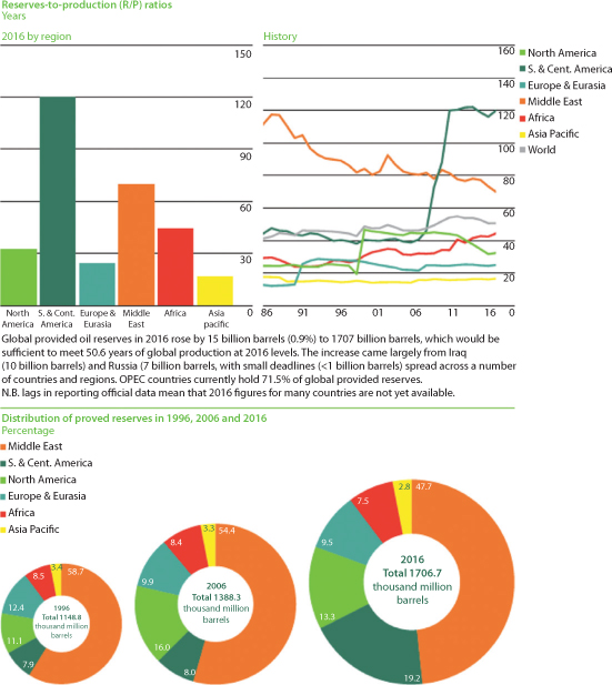
Figure 9.14 Production/reserve ratio for various countries (From BP, 2018).
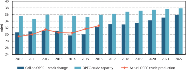
Figure 9.15 Crude oil production continues to rise overall (From EIA, 2017).
Table 9.2 shows total oil reserve as well as reserve/production ratio of top oil producing countries. Each country is marked for its need for EOR. Note that the EOR need does not imply suitability nor does it mean that other countries would not benefit from an EOR scheme.
Table 9.2 Summary of proven reserve data as of (Dec) 2016 And related reserve/production ratios (from islam et al., 2018).
| — | Country | Reserves 109 bbl (2012) |
Reserves 109 bbl (2016) |
Reserve/Production Ratio Years (2012) |
Reserve/Production Ratio Years (2016) |
| 1 | Venezuela | 296.5 |
300.9 |
387 |
341.1 |
| 2 | Saudi Arabia | 265.4 |
266.5 |
81 |
59 |
| 3 | Canada | 175 |
171.5 |
178 |
105 |
| 4 | Iran | 151.2 |
158.4 |
101 |
94.1 |
| 5 | Iraq | 143.1 |
153 |
163 |
93.5 |
| 6 | Kuwait | 101.5 |
101.5 |
121 |
88 |
| 7 | United Arab Emirates | 136.7 |
97.8 |
156 |
65.5 |
| 8 | Russia | 80 |
109.5 |
22 |
26.5 |
| 9 | Kazakhstan | 49 |
30 |
55 |
49 |
| 10 | Libya | 47 |
48.4 |
76 |
310 |
| 11 | Nigeria | 37 |
37.1 |
41 |
49.3 |
| 12 | Qatar | 25.41 |
25.2 |
63 |
36.3 |
| 13 | China | 20.35 |
25.7 |
14 |
17.5 |
| 14 | United States | 26.8 |
48 |
10 |
10.5 |
| 15 | Angola | 13.5 |
11.6 |
19 |
17.5 |
| 16 | Algeria | 13.42 |
12.2 |
22 |
21.1 |
| 17 | Brazil | 13.2 |
12.6 |
17 |
13.3 |
These numbers are only approximations. Uncertainty in reserve calculations comes from the fact the technology is evolving, both in recovery techniques and delineation of reservoirs. For instance, different estimates may or may not include oil shale, mined oil sands or natural gas liquids. Yet others would not include basement reservoirs in the calculation. In addition, proven reserves include oil recoverable under current economic conditions, which are variable depending on the overall state of economy and other factors of a country. The case in point is Canada’s proven reserve that increased suddenly in 2003 when the oil sands of Alberta were seen to be economically viable. Similarly, Venezuela’s proven reserves jumped in the late 2000 s when the heavy oil of the Orinoco was judged economic. When USA made great advances in recovering unconventional oil and gas in 2008, the US reserve increased significantly. Environmental concerns add to those uncertainties, particularly because those concerns are also a part of the political decisions.
Proven wet natural gas reserves increased in each of the five largest natural gas producing states (Texas, Wyoming, Louisiana, Oklahoma, and Pennsylvania) in 2011. Pennsylvania’s proven natural gas reserves, which more than doubled in 2010, rose an additional 90 percent in 2011, contributing 41 percent of the overall U.S. increase. Combined, Texas and Pennsylvania added 73 percent of the net increase in U.S. proved wet natural gas reserves. Expanding shale gas developments in these and other areas, particularly the Pennsylvania and West Virginia portions of the Marcellus formation in the Appalachian Basin, drove overall increases.
In terms of technical recoverability, both oil and gas reserves changed over the last decade. Figure 9.17 shows how technical recoverability has changed for both oil and gas reserves in USA. Even with reduced aggressive research, technological developments in various aspects of petroleum engineering made it possible to upgrade the reserve estimates. This decline has been accompanied with increasing sulfur content of US crude. Figure 9.18 shows general trends in sulfur content of crude oil in USA.
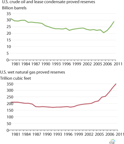
Figure 9.16 USA reserve variation in recent history (From EIA, 2018).

Figure 9.17 Technically recoverable oil and gas reserve in USA (From Islamet al., 2018).
Figure 9.18 Sulfur content of USA crude over last few decades (from EIA, 2018).
Figure 9.19 shows API gravity decline in USA crude. Together Figure 9.18 and 9.19 show that the overall quality of USA crude is declining. Figure 9.20 shows both API gravity and sulfur content of crude oil from around the world. Light and sweet crude oil is the most desirable. However, any change of the quality of the crude implies both economic and technological drain on the crude oil. Light sweet grades are desirable because they can be processed with far less sophisticated and energy-intensive processes/refineries. The figure shows select crude types from around the world with their corresponding sulfur content and density characteristics. One particular advantage of certain EOR techniques is in situ upgrading of in situ oil. While no data is available on the quality of oil recovered with EOR as compared to the same without EOR, it is reasonable to assume that in situ upgrading would improve the quality of produced oil.
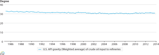
Figure 9.19 Declining API gravity of USA crude oil.
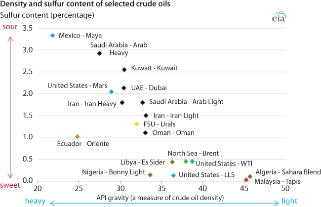
Figure 9.20 World-wide crude oil quality (From Islam et al., 2018).
The selected crude oils in the Figure 9.20 shows the ‘sweetness’ of various crude oils from around the world. These grades were selected for the recurrent and recently updated EIA report, “The Availability and Price of Petroleum and Petroleum Products Produced in Countries Other Than Iran.”
9.5 Current Status of Greenhouse Gas Emissions
It is a fact that industrial activities, especially related to the burning of fossil fuels, are major contributors of global greenhouse gas emissions – the gases that are not assimilated with the ecosystem. Climate change due to anthropogenic greenhouse gas (GHG) emissions is a growing concern for the global society, although scientists are not certain about the source of the poisoning status of the GHG. Ever since 1990s, the Intergovernmental Panel on Climate Change (IPCC) has been maintaining the position that the global warming of the last 60 years is due largely to human activity and the CO2 emissions that arise when burning fossil fuels. It has been reported that the CO2 level now is at the highest point in 125,000 years (Service 2005). Approximately 30 billion tons of CO2 are released from fossil fuel burning each year. The CO2 concentration level in the atmosphere traced back to 1750 was reported to be 280 ± 10 ppm (IPCC, 2001). It has risen continuously since then, and the CO2 level reported in 1999 was 367 ppm. The present atmospheric CO2 concentration level has not been exceeded during the past 420,000 years (IPCC 2001; Houghton et al. 2001; Houghton 2004). The latest 150 years have been a period of global warming (Figure 9.21). Global mean surface temperatures have increased 0.5–1.0 F since the late 19th century. The 20th century’s 10 warmest years all occurred in the last 15 years of the century. Of these, 1998 was the warmest year on record. Sea level has risen 4–8 inches globally over the past century, and worldwide precipitation over land has increased by about one percent. The industrial emissions of CO2 consist of process emissions and production emissions. Coal mining, oil refining, gas processing, petroleum fuel combustion, pulp and paper, ammonia, petroleum refining, iron and steel, aluminum, electricity generation, and cement production are the major industries responsible for producing various types of greenhouse gases. Besides these industrial sources, the transportation sector also contributes a large share of greenhouse gases.

Figure 9.21 Human-induced warming reached approximately 1 °C above pre-industrial levels in 2017. At the present rate, global temperatures would reach 1.5 °C around 2040 (From IPCC Panel, 2018).
Global mean surface temperatures have increased 0.5–1.0 F since the late 19th century. The 20th century’s 10 warmest years all occurred in the last 15 years of the century. Of these, 1998 was the warmest year on record. Sea level has risen 4–8 inches globally over the past century, and worldwide precipitation over land has increased by about one percent. The industrial emissions of CO2 consist of process emissions and production emissions. Coal mining, oil refining, gas processing, petroleum fuel combustion, NASA, 2018, website https://climate.nasa.gov/climate_resources/24/graphic-the-relentless-rise-of-carbon-dioxide/pulp and paper, ammonia, petroleum refining, iron and steel, aluminum, electricity generation, and cement production are the major industries responsible for producing various types of greenhouse gases. Besides these industrial sources, the transportation sector also contributes a large share of greenhouse gas emissions. Greenhouse gas emissions from bio-resources are also significant. However, the National Energy Board of Canada does not consider CO2 from biomass as contribution to greenhouse problems (Hughes and Scott 1997). The justification emerges from the fact that greenhouse gas emissions from bio-resources, such as fuel wood, agricultural waste, and charcoal, are carbon neutral because plants synthesize this CO2. However, if various additives are added during the production of fuel, such as pellet making and charcoal production, the CO2 produced is no longer carbon neutral. For instance, pellet making involves the addition of binders such as carbonic additives, coal, and coke breeze, which all emit carcinogenic benzene as a major aromatic compound (Chhetri et al. 2006). The CO2 contaminated with such chemical additives is not favored by plants for photosynthesis, and, as a result, CO2 will accumulate in the atmosphere. Moreover, deforestation, especially the unsustainable harvesting of biomass due to urbanization or so as to fulfill the industrial biomass requirement, also results in net CO2 emission from bio-resources. The worldwide CO2 emissions from the consumption of fossil fuels amounted to 24,409 million metric tons in 2002, and it is projected to reach to 33,284 million metric tons in 2015 and 38,790 million tons in 2025 (IEO 2005). The worldwide CO2 production from consumption and flaring of fossil fuels in 2003 was 25,162.07 million metric tons. The U.S. alone had a share of 5802.08 million tons of CO2 emission in 2003 (IEA 2005). The variation of CO2 concentrations at different time scales is presented in Figure 9.22. This figure shows the increase in CO2 emissions exponentially after 1950. However, present methodology does not classify CO2 based on its source. Industrial activities during this period also went up exponentially. Because of this industrial growth and extensive use of fossil fuels, the level of “industrial” CO2 emissions increased sharply. The worldwide supply of oil in 1970 was approximately 49 million barrels per day, but the supply has increased to approximately 84 million barrels per day (EIA 2006). At the same time, the level of “natural” CO2, which comes by burning biomass, went down due to deforestation. is not correct in terms of its impacts on global warming. NOAA (2005) defined the annual mean growth rate of CO2 as the sum of all CO2 added to and removed from the atmosphere by human activities and natural processes during a year. Natural CO2 cannot be the same as that of industrial CO2 and should be examined separately(NASA, 2018).
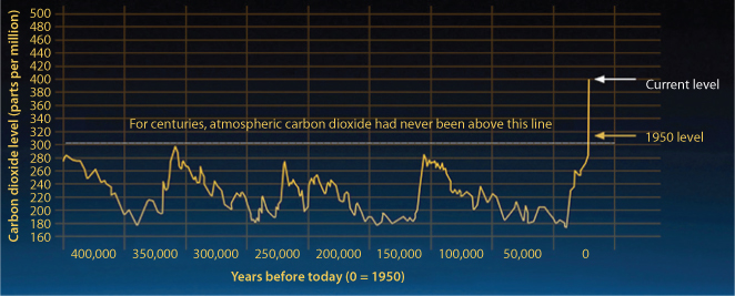
Figure 9.22 Variation in atmospheric CO2 concentration (NASA, 2018).
Figure 9.23 shows historical temperature data whereas Figure 9.24 shows historical CO2 concentration data. It is always contentious to report data from ancient past. Often, ancient air bubbles trapped in ice enable us to collect data on ancient time, however, the scientific validity and the level of representation of these data are questionable and certainly do not support the notion that these numbers can be used to calibrate historical events. Nevertheless, those data have been used to claim that the levels of carbon dioxide (CO2) in the atmosphere are higher than they have been at any time in the past 400,000 years. During ice ages, CO2 levels were around 200 parts per million (ppm), and during the warmer interglacial periods, they hovered around 280 ppm. In 2013, CO2 levels surpassed 400 ppm for the first time in recorded history. This continuous increase in CO2 shows a remarkably constant relationship with fossil-fuel burning, and can be well accounted for based on the simple premise that about 60 percent of fossil-fuel emissions stay in the air. At this rate, alarmists suggest that business-as-usual rate with the chemicals added to the refining process, CO2 will continue to rise to levels of order of 1500 ppm. The atmosphere would then not return to pre-industrial levels even tens of thousands of years into the future. This graph not only conveys the scientific measurements, but it also underscores the fact that humans have a great capacity to change the climate and planet. Tue most recent EIA report (2018) shows how climate change concerns and specifically greenhouse gas emissions have been instrumental in determining future energy outlook and regulatory policies. Regulators and investment companies been pushing energy companies to invest in technologies that are less GHG-intensive. Federal government grants are often linked to environmental aspects of petroleum engineering. Even within the petroleum industry, the focus has shifted toward mitigation of greenhouse gases.

Figure 9.23 Temperature fluctuations since 1880.
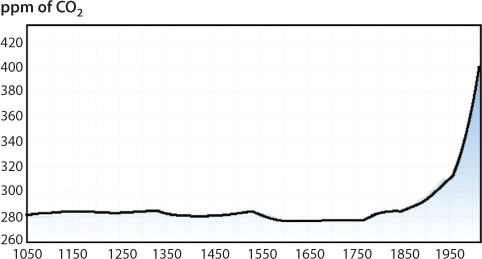
Figure 9.24 Historical concentration of CO2.
Figure 9.25 shows CO2 emissions per sector. On average, energy-related CO2 emissions in the Reference case decline by 0.2 percent per year from 2005 to 2040, as compared with an average increase of 0.9 percent per year from 1980 to 2005. Reasons for the decline include: an expected slow and extended recovery from the recession of 2007–2009; growing use of renewable technologies and fuels; automobile efficiency improvements; slower growth in electricity demand; and more use of natural gas, which is less carbon-intensive than other fossil fuels. In the Reference case, energy-related CO2 emissions in 2020 are 9.1 percent below their 2005 level. Energy-related CO2 emissions total 5,691 mil- lion metric tons in 2040, or 308 million metric tons (5.1 per- cent) below their 2005 level.

Figure 9.25 Past performance and future projections of greenhouse gases by sector. (million metric tons) (DOE/EIA, 2013)
Figure 9.25 through 9.27 show more recent data from EIA (2018). Energy-related CO2 emissions from the industrial sector grow the most on both an absolute and relative basis—0.6% annually—from 2017 to 2050 in the Reference case. Natural gas has the largest share of both energy and CO2 emissions in the industrial sector throughout the projection period. The relatively low cost of natural gas leads to further increases in usage and emissions. Even though the 2008 European gas crisis bolstered natural price, it still remains low on the basis of energy output per mass. Electric power sector CO2 emissions are relatively flat in the Reference case through 2050 as a result of favorable market conditions for natural gas and supportive policies for renewables compared with coal. Note that this scenario emerges from policies during the Obama era. After 2017, significant policy changes have been made particularly in diminishing credits for renewable energy and renewed emphasis on coal usage. Commercial sector emissions grow at a rate of 0.1% annually from 2017 to 2050, as higher energy use in the sector is only partially offset by efficiency gains. CO2 emissions in the residential and transportation sectors both decline by 0.2%/year over the projection period. Natural gas emissions grow at an annual rate of 0.8%, while petroleum and coal emissions decline at annual rates of 0.3% and 0.2%, respectively. Petroleum emissions rise in each of the final 13 years of the projection period, when increased vehicle usage outweighs efficiency gains.
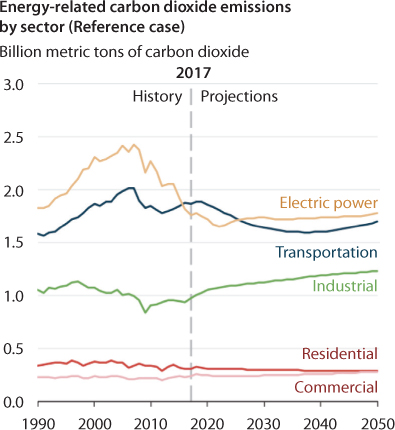
Figure 9.26 Carbon dioxide emission by sectors (EIA, 2018).

Figure 9.27 Carbon dioxide emission for various fossil fuels (EIA, 2018).
As can be seen from Figure 9.28, the total U.S. energy production increases by about 31% from 2017 through 2050 in the Reference case, led by increases in the production of renewables other than hydropower, natural gas, and crude oil (although crude oil production only increases during the first 15 years of the projection period). The contribution of so-called renewable energy is estimated through pre-Trump era thrust. However, this may likely to change. Recent announcement of President Trump that coal energy would be revived fuels the speculation that the energy outlook in new future will change toward more usage of fossil fuels (The Guardian, 2018). Trump’s new approach is expected to reduce carbon dioxide emissions from power plants by up to 1.5% by 2030. Although the EPA claims that such targets are achievable due to the usage of more effective power plants, the left remains unconvinced and the New York Attorney General vowed to sue the federal government over the deregulation plan.
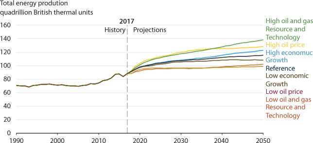
Figure 9.28 Projection relies on technology (From EIA Report, 2018).
Projected U.S. energy production is closely tied to assumptions about resources, technology, and prices, which is evident in side cases that vary these assumptions. However, the range of total production is bounded by the resource cases, which address the uncertainty in U.S. oil and natural gas resources and technology. The High Oil and Gas Resource and Technology case (Figure 9.28) assumes higher estimates than the Reference case of unproved Alaska resources; offshore Lower 48 resources; and onshore Lower 48 tight oil, tight gas, and shale gas resources. This side case also assumes lower costs of producing these resources and faster technology improvement. The Low Oil and Gas Resource and Technology case assumes the opposite. The High Oil Price case reflects the impact of higher world demand for petroleum products, lower Organization of the Petroleum Exporting Countries (OPEC) upstream investment, and higher non-OPEC exploration and development costs. The Low Oil Price case assumes the opposite.
This projection does not include latest Trump initiative regarding ANWR (USA Today, 2018). In this initiative, the Federal Register will start the environmental review process for setting up an oil and gas leasing program in the refuge’s 1.5-million-acre coastal plain. The review will help identify potential environmental issues related to the development, production and transportation of oil and gas in and from the coastal plain.
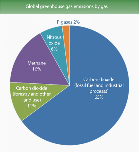
Figure 9.29 Greenhouse emissions of gas (Source: IPCC 2014).
At the global scale, the key greenhouse gases emitted by human activities are:
- Carbon dioxide (CO2) Fossil fuel use is the primary source of CO2. CO2 can also be emitted from direct human-induced impacts on forestry and other land use, such as through deforestation, land clearing for agriculture, and degradation of soils. Likewise, land can also remove CO2 from the atmosphere through reforestation, improvement of soils, and other activities. However, currently, there is no mechanism to identify and quantify contributions from different individual sources.
- Methane (CH4): Agricultural activities, waste management, energy use, and biomass burning all contribute to CH4 emissions.
- Nitrous oxide (N2O): Agricultural activities, such as fertilizer use, are the primary source of N2O emissions. Fossil fuel combustion also generates N2O.
- Fluorinated gases (F-gases): Industrial processes, refrigeration, and the use of a variety of consumer products contribute to emissions of F-gases, which include hydrofluorocarbons (HFCs), perfluorocarbons (PFCs), and sulfur hexafluoride (SF6).
- Electricity and Heat Production (25% of 2010 global greenhouse gas emissions): The burning of coal, natural gas, and oil for electricity and heat is the largest single source of global greenhouse gas emissions.

Figure 9.30 Source: IPCC (2014) on global emissions from 2010.
- Industry (21% of 2010 global greenhouse gas emissions): Greenhouse gas emissions from industry primarily involve fossil fuels burned on site at facilities for energy. This sector also includes emissions from chemical, metallurgical, and mineral transformation processes not associated with energy consumption and emissions from waste management activities. (Note: Emissions from industrial electricity use are excluded and are instead covered in the Electricity and Heat Production sector.)
- Agriculture, Forestry, and Other Land Use (24% of 2010 global greenhouse gas emissions): Greenhouse gas emissions from this sector come mostly from agriculture (cultivation of crops and livestock) and deforestation. This estimate does not include the CO2 that ecosystems remove from the atmosphere by sequestering carbon in biomass, dead organic matter, and soils, which offset approximately 20% of emissions from this sector.2
- Transportation (14% of 2010 global greenhouse gas emissions): Greenhouse gas emissions from this sector primarily involve fossil fuels burned for road, rail, air, and marine transportation. Almost all (95%) of the world’s transportation energy comes from petroleum-based fuels, largely gasoline and diesel.
- Buildings (6% of 2010 global greenhouse gas emissions): Greenhouse gas emissions from this sector arise from onsite energy generation and burning fuels for heat in buildings or cooking in homes. (Note: Emissions from electricity use in buildings are excluded and are instead covered in the Electricity and Heat Production sector.)
- Other Energy (10% of 2010 global greenhouse gas emissions): This source of greenhouse gas emissions refers to all emissions from the Energy sector which are not directly associated with electricity or heat production, such as fuel extraction, refining, processing, and transportation.
Figure 9.31 shows Global carbon emissions from fossil fuels have significantly increased since 1900. Since 1970, CO2 emissions have increased by about 90%, with emissions from fossil fuel combustion and industrial processes contributing about 78% of the total greenhouse gas emissions increase from 1970 to 2011. Agriculture, deforestation, and other land-use changes have been the second-largest contributors.

Figure 9.31 Trends in Global Emissions (From Boden et al., 2017).
Emissions of non-CO2 greenhouse gases have also increased significantly since 1900. It is in keeping with globalization efforts starting with Green Revolution in early 19th century.
As can be seen from Figure 9.32, in 2014, the top carbon dioxide (CO2) emitters were China, the United States, the European Union, India, the Russian Federation, and Japan. These data include CO2 emissions from fossil fuel combustion, as well as cement manufacturing and gas flaring. Together, these sources represent a large proportion of total global CO2 emissions.
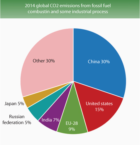
Figure 9.32 Emissions by Country (Source: Boden et al., 2017).
Emissions and sinks related to changes in land use are not included in these estimates. However, changes in land use can be important: estimates indicate that net global greenhouse gas emissions from agriculture, forestry, and other land use were over 8 billion metric tons of CO2 equivalent, or about 24% of total global greenhouse gas emissions. In areas such as the United States and Europe, changes in land use associated with human activities have the net effect of absorbing CO2, partially offsetting the emissions from deforestation in other regions. We have seen in Chapter 4, even the use of chemical fertilizer, pesticide, or GMO will affect the quality of CO2 permanently, thus skewing the impact curve away from fossil fuel usage.
9.5.1 CO2 Release to the Atmosphere
Some recent studies reported that the human contribution to global warming is negligible (Khilyuk and Chilingar 2004). The global forces of nature, such as solar radiation, outgassing from the ocean and the atmosphere, and microbial functions, are driving the Earth’s climate (Khilyuk and Chilingar 2006). These studies showed that the CO2 emissions from human-induced activities are far less in quantity than the natural CO2 emissions from ocean and volcanic eruptions. Others use this line of argument to demonstrate that the cause of global warming is, at least, a contentious issue (Goldschmidt 2005). These studies fail to explain the differences between natural and human-induced CO2 and their impacts on global warming. Moreover, the CO2 from the ocean and natural forest fires were a part of the natural climatic cycle even when no global warming was noticed. All the global forces mentioned by Khilyuk and Chilingar (2006) are also affected by human interventions. For example, more than 70,000 chemicals used worldwide for various industrial and agricultural activities are exposed, in one way or another, to the atmosphere or ocean water bodies, therefore contaminating the natural CO2. The CO2 produced from fossil fuel burning is not accepted by plants for their photosynthesis, and for this reason, most organic plant matters are depleted in carbon ratio δ13C (Farquhar et al. 1989; NOAA 2005). Finally, the notion of “insignificant” has been used in the past to allow unsustainable practices, such as the pollution of harbors, commercial fishing, and the massive production of toxic chemicals that were deemed to be “magic solutions” (Khan and Islam 2006). Today, banning chemicals and pharmaceutical products has become almost a daily affair (Globe and Mail 2006; New York Times 2006). None of these products were deemed “significant” or harmful when they were introduced. Khan and Islam (2007) have catalogued an array of such ill-fated products that were made available in order to “solve” a critical solution (Environment Canada 2006). In all these engineering observations, a general misconception is perpetrated; that is, if the harmful effect of a product can be tolerated in the short-term, the negative impact of the product is “insignificant.”
After a slowdown in growth, global CO2 emissions stalled in 2015. This was the year that ended with the signing of the landmark Climate Change Agreement in Paris by 194 countries and the EU, at the COP21 (EC-CLIMA, 2016). In preparation of the Paris Agreement, countries submitted their Intended Nationally Determined Contributions (‘INDCs’), outlining their post 2020 climate actions, and top emitters China and the United States set an example by effectively reducing their CO2 emissions over 2015 by 0.7% and 2.6%, respectively, compared to 2014 levels. Also, emissions in the Russian Federation and Japan decreased by 3.4% and 2.2%, respectively. However, these decreases were compensated for by increases in India and the European Union of 5.1% and 1.3%, respectively, and in a large group of almost 200 smaller countries that, together, accounted for 9% of global CO2 emissions. In 2015, this yielded a total amount in globally emitted CO2 emitted of 36.2 billion tonnes – virtually the same level as in 2014 (Figure 9.33). In this figure, Other OECD countries G20 include Australia, Canada, Mexico, South Korea and Turkey. Other G20 countries include Argentina, Brazil, Indonesia, Saudi Arabia and South Africa, Turkey. Other large countries include Egypt, Iran, Kazakhstan, Malaysia, Nigeria, Taiwan, Thailand and the Ukraine.

Figure 9.33 Global CO2 emissions per region from fossil-fuel use and cement production (IPCC, 2016).
The calculated trend in the global total is –0.1%. Since global population growth is 1.2% per year, stalling of global emissions means per definition a 1.2% annual decrease in global per capita CO2 emissions; that is, 4.9 tonnes CO2/capita in 2015 and 5.0 tonnes in 2014. The stalling of global emissions is no surprise, as this is in line with the slowing trend in annual emission growth over the past three years, starting from 2.0% in 2013 to 1.1% in 2014 and further down to –0.1% in 2015. A similar trend of declining growth in global emissions could also be seen from 2010 to 2012, starting from 5.7% down to 0.7%. It is debatable whether the plateaued emission level will continue and results from structural changes (Jackson et al., 2016; Qi et al., 2016; Green and Stern, 2016).
This global emission is often attributed to specific measures taken by companies and countries. As pointed out by Sullivan (2017), most companies have developed the management systems and processes necessary to manage their GHG emissions and related business risks effectively. He reported that companies in developed countries have clear management accountabilities for environmental and/or climate change issues (93% publish this information), publish environmental and/or climate change policies (92%) and GHG emissions inventories (90%), and provide at least some information on their perceptions of the risks and opportunities presented by climate change (86%).
In 2009, a stronger global downward trend of –1.0% was recorded, compared to 2008 levels, but this was due to the global economic downturn and not related to specific actions taken up by various countries. This correlation of greenhouse gas emission with GDP has been the hallmark of current civilization (Islam et al., 2018a). However, the more recent trend of the stalling in emissions is not coupled with the GDP trend, as global GDP kept up with an annual growth of 3.0% in 2015 compared to 2014. A more structural change with a shift away from carbon-intensive activities, particularly in China but also in the United States, contributed considerably to this trend. The IEA estimates that in 2015 global investment in energy efficiency increased by 6% (IEA, 2016). Changes in fossil fuel mix and renewably energy Global primary energy consumption increased in 2015 by 1.0%, which was similar to 2014 but well below the 10 year annual average of 1.9%, even though fossil fuel prices fell in 2015 in all regions (BP, 2016).
Coal consumption, globally, decreased in 2015 by 1.8%. Apart from the recession in 2009, these global annual changes represented the lowest growth levels since 1998. Global oil and natural gas consumption increased by 1.9% and 1.7%, respectively. These shifts in energy production and consumption had major effects on the fuel mix. The shift in the fossil fuel mix from coal to oil and natural gas, in part, resulted from lower regional fuel prices. The largest decreases in coal consumption were seen in the United States and China, partly counterbalanced by increases in India and Indonesia.
Figures 9.34 and 9.35 show coal consumption and production, respectively world proved coal reserves are currently sufficient to meet 134 years of global production, much higher than the R/P ratio for oil and gas. By region, Asia Pacific holds the most proved reserves (41% of total), split mainly between Australia, China and India. The US remains the largest single reserve holder (24.2% of total).

Figure 9.34 Coal consumption in 2017 by regions (BP, 2018).
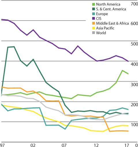
Figure 9.35 Coal production by regions (BP, 2018a).
For oil consumption, the largest increases were in China, India and United States. The global increase in the use of natural gas was mainly due to increased consumption in the United States and the European Union, with smaller increases in Iran and China, partly compensated for by decreased natural gas use, in particular in the Russian Federation and the Ukraine, as well as in Japan and South Korea (BP, 2016). Of the non-fossil fuel energy sources, nuclear energy increased by 1.3% and hydropower by 1.0%, resulting in respective shares of 4.4% and 6.8% in global primary energy consumption and 10.7% and 16.4% in total global power generation. Considerable efforts to increase other renewable power generation, notably wind and solar energy, resulted in a 15.2% increase in 2015, for the 12th consecutive year with double-digit growth, now providing almost 6.7% of global power generation, up from 3.5% in 2010. In 2015 their share increased to 2.8% of the total primary energy consumption, a doubling since 2010 (BP, 2016). Still, the remaining two thirds (66.2%) of global electricity are generated by fossil-fuel-fired power stations, which is a 0.9 percentage point down from 2014 and the lowest share since 2002. The share of fossil fuels in global primary energy consumption was 86% in 2015, calculated by using a substitution method for nuclear and renewable energy, assuming a 38% conversion efficiency (the average for OECD thermal power generation). 2015 by far the warmest year on record As for the weather, the US National Oceanic and Atmospheric Administration (NOAA) recorded 2015 as the hottest year since records began in 1880. Figure 9.36 shows regional energy demand during 1970, projected through 2040.
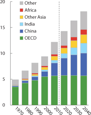
Figure 9.36 Regional energy demand (From BP, 2018).
In addition, the 16 warmest years ever recorded are in the 1998–2015 period. The year 2015 was characterised by one of the strongest El Niños in history, and with record high ocean temperatures, globally (with annually averaged ocean surface temperature around the world of 0.74 C higher than the average over the 20th century). The global land temperature for 2015 was 1.33 C above the 20th century average, surpassing the previous records of 2007 and 2010 by 0.25%, the largest margin by which an annual global land surface temperature has been broken (NOAA, 2016a). Most regions experienced record high temperatures. Europe experienced relatively mild winter months in 2015, but saw 3% more so-called Heating Degree Days than the very mild winter in 2014. Heating Degree Days (HDDs) are an indicator of the demand for space heating (EIA, 2016f). The United States and Russia benefited from a milder winter in 2015 than in 2014, and recorded 9% fewer HDDs that year (NOAA, 2016a). This led to the usage of less amount of heating fuel. A drop in natural gas consumption can be associated with the 9% drop in demand for space heating in the United States and Russia, as well as in many other countries such as Canada, Japan and South Korea. In summary, the six largest emitting countries/regions in 2015 were:
- China (with 29% share in the global total),
- the United States (14%),
- the European Union (EU-28) (10%),
- India (7%), the Russian Federation (5%) and
- Japan (3.5%)
Regional CO2 emission trends differed strongly between countries, in particular, between the top six emitting countries and the European Union, which accounted for two thirds of total global emissions (Figure 9.37). In China and the United States, emissions decreased (by 0.7% and 2.6%, respectively) after a slight increase (0.9%) in 2014, compared to 2013, whereas the European Union saw an increase (1.3%) in 2015, compared to 2014, after the large decrease in the previous year (5.4%). India’s emission growth continued, with 5.1% in 2015, compared to 2014, while emissions continued to decrease in Russia and Japan (by 3.4% and 2.2%, respectively). Of particular importance are large countries with emerging economies, such as India, which is still characterised by relatively low per capita CO2 emissions of 1.9 tonnes CO2/cap per year (17% higher than the average per capita CO2 emissions of the nearly 200 smallest and poorest countries, but still 60% below the global annual average of 4.9 tonnes CO2/capita), in combination with a large population and relatively rapidly increasing human activities. If India and the European Union were to continue their average annual change (6.8% increase per year for India and a decrease of1.9% per year for the European Union (averaged rates for 2006–2015)), then India would surpass the European Union by 2020. However, the population of India would be nearly three times that of EU-28.

Figure 9.37 CO2 emissions from fossil-fuel use and cement production in the top five emitting countries and European Union (Source: NOAA 2016).
Indonesia (currently with a share of 1.4% of the global total) showed a 4.0% increase in emissions in 2015, compared to 2014.
Of the global CO2 emission, coal-fired power plants account for one-third of global CO2 emissions. Recent trends in the fossil fuel mix with shifts from coal to natural gas, and vice versa, in the United States, China and Europe, are very relevant for the overall trend in CO2 emissions. IEA data for 2013 show that global coal combustion was responsible for 46% of CO2 emissions from fossil fuel combustion, with 31 percentage points emitted from coal-fired power plants. Since coal emits more CO2 per unit of energy than do oil and natural gas, many NGOs promote phasing out coal use in power generation, because of its large share in global CO2 emissions and since coal-fired power plants have long technical lifetimes of several decades. Among the top 4 emitting countries and the European Union, coal-fired power plants also have high but variable shares in national CO2 emissions: 48% for China, 31% for the United States, 28% for the European Union and 47% for India. However, the industry continues to build new coal-fired power plants, at a rapid pace, also in countries with an overcapacity. Utilisation rates decreased since 2005 in the top 4 emitting countries and the EU-28, to around 50% to 55%, and in India to around 65%. In China, the average coal-fired power plant ran at about 49% of its capacity in 2015. Over the course of 2015, coal-fired power plant construction activities were very different in China, compared to those in the rest of the world. In China there was an increase of 21.7 GW, whereas all other countries collectively decreased construction activities by 13.7 TW. A similar difference could be observed for the preconstruction coal plant pipeline. Since 2010, new coal-fired power plants have been built in 33 countries, totalling about 473.4 TW, of which in China and India 208 TW and 102 TW, respectively. These two countries now account for 85% of all new coal-fired power plants. Other countries, each with additions of more than 1 TW in 2015, were in decreasing order: Germany, Vietnam, Indonesia, the Netherlands, Turkey, Malaysia and the Russian Federation (Shearer et al., 2016).
China has been much of the focus in terms of efficiency and CO2 emissions. Figure 9.38 shows China has kept up with fuel efficiency (Figure showing the case of cars) and soon pass the efficiency of US cars. The main reason for the curbing of global CO2 emissions is the change in the world’s fossil-fuel use due to the structural change in the economy and in the energy mix of China. For the first time since 2000, China’s CO2 emissions decreased by 0.7% in 2015 and its per capita CO2 emissions by 1.2%, compared to 2014. Even though this relative change seems small, the difference corresponds to the total emissions in a country such as Greece. Several recent papers suggest coal consumption and CO2 emissions in China peaked in 2014 or 2015 (Qi et al., 2016; Korsbakken et al., 2016).
Figure 9.38 Fuel economy of new cars (BP, 2018).
This data set shows small decreases in coal consumption of 0.8% in 2014 and 1.5% in 2015 (in energy units). China’s CO2 emissions still increased by 2.0% in 2014, in particular due to increasing consumption of oil products and natural gas, and then decreased again by 0.7% in 2015. Although emissions in China, are double those of the United States, the Chinese per capita CO2 emission level (7.7 tonnes CO2/cap) remains below half that in the United States (16.1 tonnes CO2/cap). Even though China’s emissions increased extraordinarily rapidly, due to China’s fast industrialisation path during the first decade of the 21st century (on average, 10% per year between 2002 and 2011), the average annual increase over the 2012–2015 period amounted to only 3%. This – and the even decreasing emissions in 2015 – was mainly due to a decrease in coal consumption of 1.5% (BP, 2016) and increase in the share of non-fossil fuel in primary energy consumption from 10.9% to 11.8%. The latter was achieved through substantial increases in nuclear energy (29%), hydropower (5%) and other renewable energy such as wind and solar energy (21%), in 2015, compared to 2014 levels. Apart from the latter, China has an energy strategy aiming at reducing coal consumption and improving air quality. Among other things, it has put a cap on new coal mines and coal consumption, and has started countrywide carbon trading, initially with coal-fired power generation, encouraging hybrid and full electric cars as well as more energy-efficient cars and buildings (Adler, 2016). Moreover, China is also reducing excess capacity in industry (Xinhua, 2016). Decreasing CO2 emissions in the United States CO2 emissions in the United States decreased considerably with 2.6%, in 2015. This mainly resulted from a 13% drop in coal consumption (BP, 2016), which in percentage was the largest annual decrease in any fossil fuel in the United States, over the past five decades. The 12% decrease in energy-related CO2 emissions during the past decade mostly occurred in the power sector, due to a shift from coal to natural gas used for electricity generation, whereas the demand for electricity has remained rather constant since 2005 (EIA, 2016c). The large number of recent closures of coal-fired power plants have mainly been due to the new air pollution standards, which came into effect in 2015. Some operators decided that retrofitting certain coal-fired plants would be too costly and, instead, opted to shut these plants down permanently. In addition, over the last decade, fuel consumption decreased in the transport sector and, to a lesser extent, also in the residential and industrial sectors, all contributing to the decrease in CO2 emissions since 2005. In addition, focusing on the last years, while electricity consumption increased in 2013 and 2014, the demand fell in 2012 and 2015 due to relatively warm winter temperatures. As the warmer winters also significantly decreased the consumption of natural gas for space heating, it also lowered natural gas prices. The drop in gas prices and very efficient gas-fired power plants increased the appeal of natural gas for base load power production. As a result, in 2015, for the first time ever, the total in kWhs produced by gas-fired power plants was almost equal to those produced using coal.
It has been reported that CO2 emissions in the United States decreased considerably with 2.6%, in 2015. This mainly resulted from a 13% drop in coal consumption (BP, 2016), which in percentage was the largest annual decrease in any fossil fuel in the United States, over the past five decades. Figure 9.39 shows the CO2 emission for top emitting countries. The 12% decrease in energy-related CO2 emissions during the past decade mostly occurred in the power sector, due to a shift from coal to natural gas used for electricity generation, whereas the demand for electricity has remained rather constant since 2005 (EIA, 2016c). The large number of recent closures of coal-fired power plants have mainly been due to the new air pollution standards, which came into effect in 2015. Some operators decided that retrofitting certain coal-fired plants would be too costly and, instead, opted to shut these plants down permanently. In addition, over the last decade, fuel consumption decreased in the transport sector and, to a lesser extent, also in the residential and industrial sectors, all contributing to the decrease in CO2 emissions since 2005. In addition, focusing on the previous years, while electricity consumption increased in 2013 and 2014, the demand fell in 2012 and 2015 due to relatively warm winter temperatures. As the warmer winters also significantly decreased the consumption of natural gas for space heating, it also lowered natural gas prices. The drop in gas prices and very efficient gas-fired power plants increased the appeal of natural gas for base load power production. As a result, in 2015, for the first time ever, the total in kWhs produced by gas-fired power plants was almost equal to those produced using coal.
Figure 9.39 CO2 emissions from fossil-fuel use and cement production in the top 6 to 10 emitting countries.
Similarly, the European Union facing stagnation in emission reduction. After four years of decreasing emissions (by an average of 3.1% per year during 2011–2014), emissions in the European Union increased by 1.3% in 2015, compared to 2014 levels. Total EU emissions in 2015 reached 3.5 Gt CO2, about 50 Mt CO2 (the size of Sweden’s inventory) more than in 2014. In particular, in the southern European countries, Spain and Italy, emissions increased considerably (by 7% and 5%, respectively), mainly because of a 24% increase in coal consumption in Spain and an 8% increase in oil and natural gas consumption in Italy. In other countries, such as United Kingdom, Finland and Denmark emissions decreased between 4% and 10% in 2015, compared to 2014 levels. Renewable energy resources in the European Union were further supported and increased by 15% (excluding hydropower), yielding a share of 8.3% in primary energy consumption in 2015. Although, in 2015, the amount of hydropower in the European Union declined by 10% - mainly in Italy, Spain, France, Portugal and Romania - due to less favourable weather, the share of total renewable electricity increased by seven percentage points to 29% of total electricity production. Trends over the last decades Annual growth rates of global CO2 emissions continued to decrease from 2012 until they plateaued in 2015. Globally, there are also signs of a partial decoupling between CO2 emissions and GDP, which continued to increase in 2015 at 3%. Reports of previous years in this series on trends in Global CO2 emissions (Olivier et al., 2013, 2014, 2015) suggest that the small increases in annual CO2 emissions registered in 2012, 2013 and 2014, and currently estimated at 0.7%, 2.0% and 1.1%, could be signs of a permanent slowdown in the increase in global CO2 emissions. The 2015 stalling of global CO2 emissions confirms this and is evidence of emission levels being no longer coupled to a global economic recession. Moreover, after four years of relatively low growth rates, China’s growth in energy consumption and industrial production in the first three quarters of 2015 has been stalling under a continued increase in the share of renewable energy. Thus, it can be concluded that the slowdown of China’s CO2 emissions since 2012 has not been a temporary effect, but a more permanent trend, reflecting structural changes in the Chinese economy towards a less energy-intensive service and high value-added manufacturing industry, as well as a more low-carbon energy mix. On a global scale, the slowdown since 2012 is also not a temporary, short-term effect, but has so far already lasted for four years. It may also reflect structural changes in the global economy, such as improvements in energy efficiency and the energy mix of the key global players. However, further mitigation of fossil-fuel use, and in particular of coal use, will be needed for large absolute decreases in global greenhouse gas emissions, which will be necessary to substantially mitigate anthropogenic climate change, as was concluded by both the IPCC (2014a,b) and the Paris Agreement (UNFCCC, 2015). Technically, these reductions are still feasible (IPCC, 2014b; UNEP, 2014), but would need to be widely implemented very soon, if future global greenhouse gas emission levels need to remain compatible with pathways that could limit global warming to 2 C, or even 1.5 C, by the end of the 21st century, concluded that the slowdown of China’s CO2 emissions since 2012 has not been a temporary effect, but a more permanent trend, reflecting structural changes in the Chinese economy towards a less energy-intensive service and high value-added manufacturing industry, as well as a more low-carbon energy mix. On a global scale, the slowdown since 2012 is also not a temporary, short-term effect, but has so far already lasted for four years. It may also reflect structural changes in the global economy, such as improvements in energy efficiency and the energy mix of the key global players. However, further mitigation of fossil-fuel use, and in particular of coal use, will be needed for large absolute decreases in global greenhouse gas emissions, which will be necessary to substantially mitigate anthropogenic climate change, as was concluded by both the IPCC (2014a, b) and the Paris Agreement (UNFCCC, 2015). Technically, these reductions are still feasible (IPCC, 2014b; UNEP, 2014), but would need to be widely implemented very soon, if future global greenhouse gas emission levels need to remain compatible with pathways that could limit global warming to 2 C, or even 1.5 C, by the end of the 21st century. The level of uncertainty in national CO2 emissions varies between countries. In this report, they range from 5% to 10% (95% confidence interval), with the largest uncertainties concerning the data on countries with rapidly changing or emerging economies, such as Russian Federation data on the early 1990 s and data on China since the late 1990s, based on Marland et al. (1999), Tu (2011), Andres et al. (2012), Guan et al. (2012), Liu et al. (2015) and Korsbakken et al. (2016). Moreover, in general, the most recent statistics are also somewhat more uncertain for every country, since first published statistics are often subject to subsequent revisions when more detailed data become available (Olivier and Peters, 2002). For China, Wang and Chandler (2011) give a good description of the revision process for energy and GDP statistics, also in response to the two National Economic Censuses. Korsbakken et al. (2016) built on and extended the study by Wang and Chandler (2011) and compared the impact of various revisions of coal statistics by the NBS, following each of the three National Economic Censuses. For China, the Russian Federation and most other non-OECD countries, we assumed 10% uncertainty, whereas for the European Union, the United States, Japan India and other OECD countries, a 5% uncertainty was assumed. Our preliminary estimate of total global CO2 emissions in 2015 is believed to have an uncertainty of about 5%, and our estimated emission decrease of 0.1% may be accurate to within ± 0.5%.
9.5.2 Linking with GDP
Gross Domestic Product (GDP) can be considered the total value added achieved by all economic sectors, which greatly differ in terms of energy intensity, such as the power sector, energy-intensive basic materials industry, other industries, service sectors and agriculture. Moreover, household energy consumption for heating, electrical appliances and private transport is not directly coupled to GDP. Annual growth rates often greatly vary between sectors. Therefore, annual trends in GDP and total energy consumption are generally only very weakly related. Since the energy mix generally varies per sector and country, the link between global GDP and global CO2 emissions is even weaker. The relationship between the increase in annual global CO2 emissions and the annual increase in atmospheric CO2 concentrations (not included in this study) is also rather weak. This is because the net annual increase in CO2 concentrations is affected by the large inter-annual changes in CO2 emissions from forest fires and deforestation and in the amount of CO2 absorbed by vegetation, in particular by growing forests, which vary substantially depending on temperature and the amount of sunshine and precipitation. Moreover, the large absorption of atmospheric CO2 by the oceans also varies over time. These changes are larger in ‘El Nino years’, such as 2015. The IPCC’s Fifth Assessment Report (IPCC, 2014a, b) concluded that the effects of anthropogenic greenhouse gas emissions have been detected throughout the climate system and are extremely likely to have been the dominant cause of the observed warming since the mid-20th century. Cumulative emissions of carbon dioxide will largely determine global mean surface warming by the late 21st century and beyond. It would be possible, using a wide array of technological measures and changes in behaviour, to limit the increase in global mean temperature to 2 C above pre-industrial levels. There are multiple mitigation efforts that in addition to those in place today required to reduce CO2 emissions to near zero and so limit the increase in global mean temperature to 2 C above pre-industrial levels.
The Paris Agreement, which was adopted on 12 December 2015, is a global milestone for enhancing collective action and accelerating the global transformation to a low-carbon and climate-resilient society. The Paris Agreement entered into force in October 2016, after having been ratified by 55 countries, and accounts for at least 55% of global emissions. The Paris Agreement includes both mitigation and adaptation actions and the countries agreed, among other things, on the following key elements: On reducing global emissions: The target to keep the global average temperature well below 2 C above pre-industrial levels; To pursue efforts to limit the temperature increase to 1.5 C above pre-industrial levels, since this would significantly reduce risks and the impacts of climate change; The need for global emissions to peak as soon as possible, recognising that this will take longer for developing countries; To undertake rapid reductions thereafter, in accordance with best available science. On transparency, NDCs and global stock-take: Countries shall submit national climate action plans (Nationally Determined Contributions, NDCs) as contributions to the global response to climate change; – Each successive NDC will represent a progression beyond the then current NDC and reflect its highest possible ambition; – Countries shall report to each other and the public on how well they are doing on the implementation of their targets; – Countries shall track their progress towards the long-term goal, using a robust transparency and accountability system; – Countries shall, every 5 years, make a global stock take to set more ambitious targets as required by science.
9.5.3 Different Trends in the Largest Emitting Countries and Regions
The most significant introduction to the global climate change scenario is China. China’s CO2 emissions, in 2015, decreased by about 0.7%, compared to 2014. This was mainly due to a 1.5% decline in coal consumption, partly compensated for by increases in oil consumption of 6.3% and natural gas of 4.7% (all percentages in energy units, e.g. in PJ) (BP, 2016). Coal is the dominant fossil fuel in the non-transport sectors: power generation, industry, residential and services (IEA, 2015b, 2016c). China’s CO2 emissions from fossil fuel combustion, which account for about 85% of total national CO2 emissions, originated in 2013 for 83% from coal, 14% from oil products and 3% from natural gas. Although the shares of oil and natural gas are on the rise, the reliance of China on coal is one of the highest of all countries. To calculate the CO2 emissions for China from all fossil-fuel-related activities, we used IEA’s revised energy balance statistics on China (TJ with fuel consumed in each sector) for the 1990–2014 period (IEA, 2016c), which includes all detailed revisions published in May 2015 by the National Bureau of Statistics of China (NBS) for the 2000–2013 period on an aggregate level only (NBS, 2015c). For more information on how the IEA included the revised detailed energy balances of NBS, see IEA (IEA, 2016f). The very large share of coal combustion emissions in the national total was due to the large amount of coal used in the manufacturing industry (28% of the national total), whereas coal-fired power generation accounted for 48% of the national total.

Figure 9.40 Shares of greenhouse gas emissions, 2010 (IEA, 2016f). Source: CO2 fossil fuel and industrial processes: EDGAR 4.3.2 (JRC/PB, 2016, notably IEA, 2014); others: EDGAR 4.2 FT2010 (JRC/PBL 2012). In this figure, storage/removal of emissions (also known as ‘sinks’) are not shown here. This figure differs from CO2 emissions in this report: it includes CO2 emissions from forest fires and deforestation (‘Forests’) (shown in red), but excludes CO2 sinks/removals of mainly living carbon stock change. For the latter see GCP (2016). Moreover, 2010 was chosen as this is the most recent year for which EDGAR data on non-CO2 sources are presently available).
9.6 Comments on the Copenhagen Summit
Picture 9.2 shows locations of principal international events that dealt with the climate change issues. In 2011, Durban, South Africa was unique because of the fact that countries agreed to achieve an outcome that was applicable to all parties. Some argued that it was Copenhagen accord that was the first one to agree on a universal outcome. Also, most of the key elements of the Paris Agreement can be found in the Copenhagen Accord. The shift away from the binary approach to differentiation that was at the heart of the Kyoto Protocol, towards a more flexible approach that encompasses all countries is in the core of these latest agreements. With that comes the pledge to mobilize climate finance from public and private sources (with a target figure of $100 billion specified in the Paris decision text but not the agreement itself). At the end, it all boils down to channeling funds from public to private sectors and from one country to another. Copenhagen was special in the sense that it marked a new beginning of pledges in the run up and at Copenhagen covered 80% of global emissions, up from Kyoto (never more than 50% and had fallen to less than 20%), and not far below Paris (96%). For a decade, the entire world pinned hope on Kyoto protocol. Even though for some scientists it was just business as usual, for the vast majority of general public, it was supposed to offer reversal of global warming. As the developed nations came to realize the goals set for Kyoto protocol cannot be achieved, new hope was introduced in the name of Copenhagen summit.
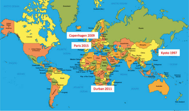
Picture 9.2. locations of various international big events regarding Climate Change.
Thanks to the transparency of the information age, it has become possible to observe the political chaos created during the Copenhagen Summit. To some extent, the world public could witness the humiliating treatment of heads of states, and thousands of high-profile representatives from various countries. On December 18, 2009, the final day of the Summit was suspended by the Danish government to hand over the principal conference room to US President Obama, where he and a select group of invitees, 16 in total, would have the exclusive right to speak. Obama’s speech failed to imply any binding commitment to environmental integrity and more importantly, undid any hope of the Kyoto Framework Protocol. He left the room after listening to a few more speakers. Among those invited to take the floor were the most industrialized countries, a number of the emerging economies and some of the least developed countries (LDC). The leaders and representatives of more than 170 only had the right to listen. From the night of December 17 to the early hours of the 18th, the prime minister of Denmark and senior U.S. representatives met with the president of the European Commission and the leaders of 27 countries in order to propose to them, on Obama’s behalf, a draft agreement which did not have the participation of any of the other leaders from the rest of the world. If sustainability means bottom-up participation, this was indeed an unsustainable move to ‘fix the climate’. During the entire night of the 18th to three in the morning on the 19th, when many heads of state had already gone, the country representatives were waiting for the re-initiation of the sessions and the closing session. Obama had meetings and press conferences all day on the 18th. The European leaders did likewise. Then they left. Then an unheard of event took place: at three in the morning on the 19th, the prime minister of Denmark convened a meeting for the closing of the Summit. Ministers, officials, ambassadors and technical personnel remained representing their countries. This move did not go unchallenged. A number of third world country representatives insisted on their voice heard. It was a remarkable move, particularly by the members of the ALBA (Bolivarian Alternative for the Americas). The following statements of Cuban, representative summarizes the nature of the Copenhagen Summit and how it offered no hope for greening the environment (Islam et al., 2010).
“The document that you affirmed on a number of occasions did not exist, Mr. President, has now appeared. We have seen versions that were circulating surreptitiously and being discussed in small secret meetings …
Cuba considers the text of this apocryphal project as insufficient and inadmissible. The goal of two degrees centigrade is unacceptable and would have incalculable disastrous consequences.
The document that you, lamentably, are presenting has no commitment whatsoever to reduced emissions of greenhouse gases …
I am aware of earlier versions that, via questionable and clandestine procedures, were being negotiated in closed corridors.
The document that you are now presenting precisely omits the already meager an insufficient key phrases that that version contained …
For Cuba, it is incompatible with the universally recognized scientific criterion which considers it urgent and unavoidable to assure levels of reduction of at least 45% of emissions by the year 2020, and a reduction of no less than 80% or 90% by 2050 …
Everything proposed around the continuation of negotiations for adopting, in the future, agreements on reductions of emissions, must inevitably include the concept of the validity of the Kyoto Protocol. Your paper, Mr. President, is the death certificate of the Kyoto Protocol, which my delegation does not accept …
The Cuban delegation wishes to emphasize the pre-eminence of the principle of ‘common but distinguished responsibilities’ as a central concept of the future negotiation process. Your paper does not say a single word about that. This draft declaration omits concrete commitments of funding and the transfer of technologies to the developing countries as part of meeting the obligations contracted by the developed countries under the United Nations Framework Convention on Climate Change The developed countries which are imposing their interests via this document, Mr. President, are evading any concrete commitment.
Mr. President, what you refer to as ‘a group of representative leaders’ is, for me, a gross violation of the principle of sovereign equality consecrated in the Charter of the United Nations.
Mr. President, I am formally asking for this declaration to be included in the final report on the work of this lamentable and shameful 15th Conference of the Parties.”
The state representatives were given only one hour to express their views. Following that hour, there came a long debate in which the delegations of the developed countries exercised heavy pressure in an attempt to make the Conference adopt the said document as the final result of their deliberations. This did not bode well with developing countries that pressed on fundamental issues, such as, (a) absence of any commitment on the part of the developed countries in terms of the reduction of carbon emissions; or, (b) funding for the nations of the South to adopt measures of mitigation and adaptation. At the end, the Conference confined itself to “taking note” of the existence of that document as the position of a group of approximately 25 countries.
The following is the draft decision that was being touted by the President of Conference:
Draft decision -/CP.15
Proposal by the President
Copenhagen Accord
The Heads of State, Heads of Government, Ministers, and other heads of delegation present at the United Nations Climate Change Conference 2009 in Copenhagen,
In pursuit of the ultimate objective of the Convention as stated in its Article 2, Being guided by the principles and provisions of the Convention, Noting the results of work done by the two Ad hoc Working Groups, Endorsing decision x/CP.15 on the Ad hoc Working Group on Long-term Cooperative Action and decision x/CMP.5 that requests the Ad hoc Working Group on Further Commitments of Annex I
Parties under the Kyoto Protocol to continue its work, Have agreed on this Copenhagen Accord which is operational immediately.
- We underline that climate change is one of the greatest challenges of our time. We emphasise our strong political will to urgently combat climate change in accordance with the principle of common but differentiated responsibilities and respective capabilities. To achieve the ultimate objective of the Convention to stabilize greenhouse gas concentration in the atmosphere at a level that would prevent dangerous anthropogenic interference with the climate system, we shall, recognizing the scientific view that the increase in global temperature should be below two degrees Celsius, on the basis of equity and in the context of sustainable development, enhance our long-term cooperative action to combat climate change. We recognize the critical impacts of climate change and the potential impacts of response measures on countries particularly vulnerable to its adverse effects and stress the need to establish a comprehensive adaptation programme including international support.
- We agree that deep cuts in global emissions are required according to science, and as documented by the IPCC Fourth Assessment Report with a view to reduce global emissions so as to hold the increase in global temperature below two degrees Celsius, and take action to meet this objective consistent with science and on the basis of equity. We should cooperate in achieving the peaking of global and national emissions as soon as possible, recognizing that the time frame for peaking will be longer in developing countries and bearing in mind that social and economic development and poverty eradication are the first and overriding priorities of developing countries and that a low-emission development strategy is indispensable to sustainable development.
- Adaptation to the adverse effects of climate change and the potential impacts of response measures is a challenge faced by all countries. Enhanced action and international cooperation on adaptation is urgently required to ensure the implementation of the Convention by enabling and supporting the implementation of adaptation actions aimed at reducing vulnerability and building resilience in developing countries, especially in those that are particularly vulnerable, especially least developed countries, small island developing States and Africa. We agree that developed countries shall provide adequate, predictable and sustainable financial resources, technology and capacity-building to support the implementation of adaptation action in developing countries.
- Annex I Parties commit to implement individually or jointly the quantified economy wide emissions targets for 2020, to be submitted in the format given in Appendix I by Annex I Parties to the secretariat by 31 January 2010 for compilation in an INF document. Annex I Parties that are Party to the Kyoto Protocol will thereby further strengthen the emissions reductions initiated by the Kyoto Protocol. Delivery of reductions and financing by developed countries will be measured, reported and verified in accordance with existing and any further guidelines adopted by the Conference of the Parties, and will ensure that accounting of such targets and finance is rigorous, robust and transparent.
- Non-Annex I Parties to the Convention will implement mitigation actions, including those to be submitted to the secretariat by non-Annex I Parties in the format given in Appendix II by 31 January 2010, for compilation in an INF document, consistent with Article 4.1 and Article 4.7 and in the context of sustainable development. Least developed countries and small island developing States may undertake actions voluntarily and on the basis of support. Mitigation actions subsequently taken and envisaged by Non-Annex I Parties, including national inventory reports, shall be communicated through national communications consistent with Article 12.1(b) every two years on the basis of guidelines to be adopted by the Conference of the Parties. Those mitigation actions in national communications or otherwise communicated to the Secretariat will be added to the list in appendix II. Mitigation actions taken by Non-Annex I Parties will be subject to their domestic measurement, reporting and verification the result of which will be reported through their national communications every two years. Non-Annex I Parties will communicate information on the implementation of their actions through National Communications, with provisions for international consultations and analysis under clearly defined guidelines that will ensure that national sovereignty is respected. Nationally appropriate mitigation actions seeking international support will be recorded in a registry along with relevant technology, finance and capacity building support. Those actions supported will be added to the list in appendix II. These supported nationally appropriate mitigation actions will be subject to international measurement, reporting and verification in accordance with guidelines adopted by the Conference of the Parties.
- We recognize the crucial role of reducing emission from deforestation and forest degradation and the need to enhance removals of greenhouse gas emission by forests and agree on the need to provide positive incentives to such actions through the immediate establishment of a mechanism including REDD-plus, to enable the mobilization of financial resources from developed countries.
- We decide to pursue various approaches, including opportunities to use markets, to enhance the cost-effectiveness of, and to promote mitigation actions. Developing countries, especially those with low emitting economies should be provided incentives to continue to develop on a low emission pathway.
- Scaled up, new and additional, predictable and adequate funding as well as improved access shall be provided to developing countries, in accordance with the relevant provisions of the Convention, to enable and support enhanced action on mitigation, including substantial finance to reduce emissions from deforestation and forest degradation (REDD-plus), adaptation, technology development and transfer and capacity-building, for enhanced implementation of the Convention. The collective commitment by developed countries is to provide new and additional resources, including forestry and investments through international institutions, approaching USD 30 billion for the period 2010. 2012 with balanced allocation between adaptation and mitigation. Funding for adaptation will be prioritized for the most vulnerable developing countries, such as the least developed countries, small island developing States and Africa. In the context of meaningful mitigation actions and transparency on implementation, developed countries commit to a goal of mobilizing jointly USD 100 billion dollars a year by 2020 to address the needs of developing countries. This funding will come from a wide variety of sources, public and private, bilateral and multilateral, including alternative sources of finance. New multilateral funding for adaptation will be delivered through effective and efficient fund arrangements, with a governance structure providing for equal representation of developed and developing countries. A significant portion of such funding should flow through the Copenhagen Green Climate Fund.
- To this end, a High Level Panel will be established under the guidance of and accountable to the Conference of the Parties to study the contribution of the potential sources of revenue, including alternative sources of finance, towards meeting this goal.
- We decide that the Copenhagen Green Climate Fund shall be established as an operating entity of the financial mechanism of the Convention to support projects, programme, policies and other activities in developing countries related to mitigation including REDD-plus, adaptation, capacity building, technology development and transfer.
- In order to enhance action on development and transfer of technology we decide to establish a Technology Mechanism to accelerate technology development and transfer in support of action on adaptation and mitigation that will be guided by a country-driven approach and be based on national circumstances and priorities.
- We call for an assessment of the implementation of this Accord to be completed by 2015, including in light of the Convention’s ultimate objective. This would include consideration of strengthening the long-term goal referencing various matters presented by the science, including in relation to temperature rises of 1.5 degrees Celsius.
APPENDIX I
Quantified economy-wide emissions targets for 2020
Annex I Parties Quantified economy-wide emissions targets for
9.6.12020
Emissions reduction in 2020 Base year
APPENDIX II
Nationally appropriate mitigation actions of developing country
Parties
Non-Annex I Actions
9.7 The Paris Agreement
The Paris Agreement was adopted by consensus on the 12 December 2015. The Agreement is a treaty under international law and is binding upon member parties. It gained notoriety over President Trump’s abandonment but recovered much of what was lost during the Nobel Prize season of 2018.
9.7.1 Connection to Nordhaus
In order to understand the Paris Agreement, one has to look into the mindset of Bill Nordhaus, the first Nobel laureate economist with ties to climate science. In a recent keynote speech on the retirement ceremony of Martin Weitzman, Nordhaus gave the title:
The Intellectual Footprint of Martin Weitzman in Environmental Economics (Stavins, 2018). He opened the speech with attribution to Weitzman, who “has changed the way we think about economics and the environment.” Nordhaus then went on to itemize Weitzman’s impressive body of work, including his series of studies on the share economy; his research on the Soviet Union and central planning; his seminal 1974 paper, “Prices vs. Quantities,” which provided fresh insight on how regulatory policy can best be leveraged to maximize public good; and his work on so-called “fat tails” and the “dismal theorem,” which questioned the value of a standard benefit-cost analysis when conditions could result in catastrophic events, even if the probability of such events is very low. Nordhaus devoted much of his talk to highlighting Weitzman’s extraordinary contributions to the field of environmental economics, in particular, the economics of climate change and climate change policy. It was Weitzman’s “revolutionary” series of papers on the ideal measures of national income, Nordhaus stated, that focused early attention on the need to take the harmful impacts of pollution into account when tabulating the gross domestic product (GDP), a concept referred to as “Green GDP.” This is a term that has been introduced as an index of economic growth with the environmental consequences of that growth factored into a country’s conventional GDP. It is an implicit way of quantifying environmental effects that are vastly intangible (Zatzman and Islam, 2007; Islam et al.,, 2018a). Green GDP is a means to monetize the loss of biodiversity, and accounts for costs caused by climate change. Some environmental experts prefer physical indicators (such as “waste per capita” or “carbon dioxide emissions per year”), which may be aggregated to indices such as the “Sustainable Development Index”. In Islam et al. (2018a), this has been included in its scientific form through consideration of intangibles – the entire time function that is ignored in conventional economic analysis.
In that keynote speech, Nordhaus stated, “Our output measures do not include pollution … They include goods like cars and services like concerts and education, but they do not include CO2 that is pumped into the atmosphere.” He explained that pollution abatement measures are often blamed for causing a drag on the economy, but aren’t credited for the health and welfare benefits they create. Of course, the implicit assumption is that modern technologies are constantly generating avenues to improve sustainability and environmental impact. In reality, each new technology covers up the negative effects that eventually show up at a later date (Islam et al., 2018a). The following quote serves as a reminder that economists and scientists alike have become a tool for justifying policies. As it was discovered only recently, the real intent behind these ‘scientific’ observation is to justify universal carbon tax (from Stavins, 2018).
“If our incomes stay the same but we are healthier, and live a year longer or ten years longer, that will not show up in the way we measure things,” Nordhaus added. “But we can apply these Weitzman techniques to value improvements in health and happiness.”
“Those who claim that environmental regulations hurt growth are completely wrong, because they are using the wrong yardstick,” Nordhaus continued. “Pollution should be in our measures of national output, but with a negative sign, and if we use green national output as our standard, then environmental and safety regulations have increased true economic growth substantially in recent years.For this important insight we applaud Martin Weitzman, a radically innovative spirit in economics.”
The ‘radically innovative technique’ of Weitzman that’s being lauded is nothing but transformation of intangibles into tangibles with a distinct role played by the economist (Weitzman, 1974). Islam et al. (2018a) critiqued this technique as a launchpad in the wrong direction, in which perception is transformed into reality with the motive of the economist hidden.
9.7.2 The Agreement
The Paris Agreement entered force and became legally binding on ratifying countries on 4 November 2016. Currently, 143 countries have ratified the Agreement (UNFCCC, 2017). Kemp (2018) gives a useful critique of the of the 2015 Paris Agreement on Climate established at the 21st Conference of the Parties (COP21) to the United Nations Framework Convention on Climate Change (UNFCCC). This Agreement had the promises of a panacea but became flat after US President Donald Trump refused to back it up much to the chagrin of vast majority of scientists that continue to peddle carbon tax and ‘carbon is the enemy’ line. The Agreement was considered inadequate to limit global warming to safe levels but it contained recommendations for ambitious emissions reductions from members. The Agreement was uniquely designed to increase action through a “ratchet mechanism” obligating countries to put forward stronger targets, political pressure and a “signal” to investors to transition towards low-carbon portfolios and activities. In general, it meant increasing the marketability of so-called renewable energy technologies in favour of making fossil fuel technologies more difficult to afford. Kemp (2018) concluded that none of the expressed intention of the Paris Agreement was logical or could be realistically implementable. The legal wording of the Paris Agreement means that no “ratchet mechanism” exists. Political pressure through a pledge and review process has rarely worked in other international agreements or in previous international efforts on climate change. The idea of international law sending an investment signal is tenuous at best, and existing evidence in renewable energy and fossil fuel markets suggests that the signal is currently not functioning. Furthermore, Kemp detected that the Paris Agreement has inbuilt delay, making the lock-in of emissions-intensive trajectories likely. Long before President Trump called it out in the following terms (Whitehouse, 2017):
Compliance with the terms of the Paris Accord and the onerous energy restrictions it has placed on the United States could cost America as much as 2.7 million lost jobs by 2025 according to the National Economic Research Associates. This includes 440,000 fewer manufacturing jobs — not what we need — believe me, this is not what we need — including automobile jobs, and the further decimation of vital American industries on which countless communities rely. They rely for so much, and we would be giving them so little.
According to this same study, by 2040, compliance with the commitments put into place by the previous administration would cut production for the following sectors: paper down 12 percent; cement down 23 percent; iron and steel down 38 percent; coal — and I happen to love the coal miners — down 86 percent; natural gas down 31 percent. The cost to the economy at this time would be close to $3 trillion in lost GDP and 6.5 million industrial jobs, while households would have $7,000 less income and, in many cases, much worse than that.
In short, the mechanisms for change designed into the Paris Agreement are unlikely to work. The Agreement as a system for changing state behaviour in a sufficient timescale is likely to fail.
In this section, we will see the real merit of this Agreement so we can proceed to study the real science behind global warming.
The Paris Agreement is not a new or unique agreement. It follows from decades of concern over climate change and all the hysteria surrounding it. In reality, the direction that was set in Kyto Protocol, which itself emerges from Framework Convention on Climate Change (UNFCCC) adopted at the Earth Summit in Rio de Janeiro in 1992. The direction set in previous Agreements became ingrained in Paris Agreement and the direction has always been away from real sustainability (Islam et al., 2018a).
The Paris Climate Agreement of 2015 is one agreement that has widely been heralded as a diplomatic success (Harvey, 2015; Rajamani, 2016). However, this is nothing new. History of modern-day technology development tells us that every new initiative has been heralded as the ultimate panacea only to discover within years it was a terrible choice, thus making way to the development of newer technologies, triggering another series of celebration (Khan and Islam, 2016).
The overarching goals of the Agreement, stated under Article 2, are to limit “increase in the global average temperature to well below 2 C above pre-industrial levels and to pursue efforts to limit the temperature increase to 1.5 C above pre-industrial levels”. This is later elaborated on in Article 4, which aims to achieve “balance between anthropogenic emissions by sources and removals by sinks of greenhouse gases in the second half of this century”. Of course, this cannot be achieved unless a zero emission mode is utilized (Rockström et al., 2017). Zero emissions, on the other hand cannot be achieved without using zero-waste system. Yet, zero-waste has been considered as an oxymoron in the post Kelvin era of engineering (Khan and Islam, 2016). Then, one must ask where did this number 2 C come from? As we have seen in the previous section this value has no scientific basis. Without regards to these clearly illogical feature of the fundamental basis, the Paris Agreement establishes a pledge and review process that requires countries to put forward pledges every 5 years, with correlated reviews called “global stocktakes”. The pledges for national climate action or nationally determined contributions (NDCs) under the Agreement, however, are not legally binding. Instead, they are simply political commitments (Bodansky, 2015), subject to changes as a political regime changes.
The pledge and review cycles of Paris are depicted in Table 9.1. The first submission of new pledges will occur in 2025 and will be proceeded by the first global stocktake in 2023. These stocktakes will account for and review the cumulative efforts of countries under the Agreement and estimate the temperature rise and greenhouse gas concentration the world is tracking towards. It will also review collective progress in terms of international financing of climate efforts and adaptation activities. The next stocktake will then occur in 2028, followed by a new round of pledges in 2030. The cycle will continue ad infinitum until net zero emissions (or presumably ecological collapse) is reached. However, if this outcome will not be in the right direction unless true sustainability is employed. That involves eliminating sources of unsustainability, namely the use of artificial chemicals as well as artificial energy sources.
Table 9.3 The paris agreement process (from Kemp, 2018).

The Paris Agreement hinges upon the existence of the ratchet mechanism. It is expected that the pledges and review system of the Paris Climate Agreement is intended to hinge on the use of a ratchet mechanism: a measure that forces countries to periodically ratchet up their commitments. However, the agreement does not identify the source of such a mechanism or what would inspire a country to ratchet up its commitment. The provisions of global stocktakes and the stipulation that future pledges be informed by the stocktake are part of the perceived ratcheting mechanism but are non-existent. In the meantime, stocktakes themselves are inherently weak and the need for future pledges to be “informed” by stocktakes in legal practice means little more than mere token (Kemp, 2018). The main mechanism for ratcheting is situated under Article 4.3 of the Agreement which reads “Each Party’s successive nationally determined contribution will represent a progression beyond the Party’s then current nationally determined contribution …” (UNFCCC, 2015). The wording here ambiguous and subject to speculation. Overall, there is no provision for mitigation. There is a legal argument that a small increase in international climate financing accompanied by an unchanged mitigation target could be put forward as a progression. This argument is based on the fallacy that financing is directly connected to technological advancement and that too in a sustainable fashion.
It is not a matter of adding the term ‘progression’ because even if progression in emissions cuts was required, it would be have no tooth unless any mechanism to enforce it was put in place. Also, an increase in terms of mitigation commitments could be entirely insignificant but still qualify as a progression. For instance, the Australian pledge is to reduce emissions 26–28% below 2005 levels by 2030 (Australian Government, 2015). A progression on this target could be 29–30% by 2035. It would not be a progression in terms of the rate of emissions reductions but would be an increase in absolute terms. We are thrown back to the dilemma of not having a standard. In absence of such standard, any country could put forward incremental progressions but never achieve them. Pledges under Paris are unbinding and there are no mechanisms to effectively enforce the fulfilment of legal obligations.
As pointed out by Kemp (2018), Article 4.3 can actually create perverse incentives for weaker targets. If a country believes it needs to scale-up action over time, there may be an enticement to initially put forward weaker targets. That would make both the achievement of targets and progression easier. It is politically far safer for countries to put forward weaker targets and then overachieve rather than risk more stringent goals they may not meet (Raustiala, 2005). This seems to be a typical problem that comes from the post-enlightenment era, in which good intention is banked on while recognizing that every player would act selfishly.
Some authors penned hope considering that the Paris Agreement does contain some positive traits due to the existence of two feedback mechanisms that could bolster ambition over time. The first mechanism is simple political pressure. The entire premise of a pledge and review system is that pressure from within countries and from other states can hold governments accountable to their targets (Bodansky, 2016). This is based on the belief that a pledge can be just as effective as a legal contract if the state believes its reputation and popular support will suffer if it publicly fails to meet it (Jacquet & Jamieson, 2016). Once again, this premise banks on the fallacy that a country can be selfish and selfless at the same time. In addition, the fallacy that the regular occurrence of a global stocktake every 5 years can to create political moments that can pressure governments into increasing ambition. The second mechanism is the idea of a “market message” or “investment signal “. This is the notion that long-term goals supported by pledges showcase to investors that the world is heading towards decarbonisation (van Asselt, 2016). Here, the premise that ‘carbon is the enemy’ is firmed up and then the corporations are lured into thinking there is money to be made in this decarbonisation process. This regulatory certainty in low-emissions developments and uncertainty for emissions-intensive investments is manifested in the 2018 declaration and related Nobel prize in Economics that claim that universal carbon tax would trigger both economic growth and environmental sustainability – a clear paradox. Yet, this is the very feature of Paris Agreement that was hailed by the mainstream financial authorities. Soon after the Paris Agreement, an op-ed in the Economist wrote: “Perhaps the most significant effect of the Paris agreement in the next few years will be the signal it sends to investors … after Paris, the belief that governments are going to stay the course on their stated green strategies will feel a bit better founded—and the idea of investing in a coal mine will seem more risky” (The Economist, 2015). It’s almost begging to trust the corporation to be benevolent for the reason that the government is also perceived to be acting in good faith.
Figure 9.41 is a causal loop diagram of how these two feedback mechanisms should theoretically operate. In causal loop diagrams, arrows denote a flow of influence. The “variables” (boxed and unboxed labels) are key aspects of the system under investigation. Polarities (+and –) show the nature of the relationship between variables. They are not moral judgements but simply highlight how one variable will change a connected variable. Positive signs (+) demonstrate that the direction of change of the variable at the tail of the arrow will be the same as that the head (e.g., increasing progress towards global goals increases the level of regulatory certainty). Negative polarities (–) signify the opposite: an increase in the variable at the tail of the arrow will decrease the variable at the head, and vice versa. The diagram in Figure 9.41 is simplified to showcase the main causal loops, or feedback mechanisms, that are supposed to drive climate action under the Paris Agreement.
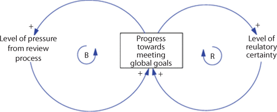
Figure 9.41 The feedbacks of Paris.
9.8 Carbon Tax: The Ultimate Goal of Climate Change Hysteria
It is no surprise that every science and technology discussion always ends with a conclusion that stipulates more government spending, which in turn monetizes any science. Long before understanding global climate change and the cause behind it, there has been a superflux of justification for more government spending. As we have seen in an earlier section, a carbon tax was sought out even during the nascent state of the Climate Change movement, culminating in the most recent declaration emboldened by Nobel prize in economics. It has always been argued that despite the uncertainties, reducing emissions makes sense, and a carbon tax is the simplest, most effective, and least costly way to do this. It is understood that a carbon tax would provide substantial new revenues which may be badly needed, especially in USA, where historically high debt-to-GDP levels, pressures on social security and medical budgets, and calls to reform taxes on personal and corporate income. Until President Trump was installed, this path to carbon tax was a given. In Canada, where liberal hold the majority, carbon tax has become a reality with the premise that: “it should not be free to pollute” (Financial Post, 2018). When such a push faced resistance, it was quickly stated that 90% of the carbon tax collected would be returned to the payers. One is left wondering what this would accomplish in term of government efficiency. Clearly, this obsession with carbon tax is aimed at helping the government more than the environment.
Ever since the Clinton era, carbon tax has been mulled by the government and also the mainstream academics, who have vested interest in increasing government revenue. The initial justification involves the elimination of selected other tax subsidies and spending programs. It is promoted that the distributional effects would be regressive but could be offset by other policy changes. The following expressed reasoning is offered (Williams III and Wichman, 2015):
- A carbon tax (taken by itself) will likely impose a small but significant long-term drag on the economy.
- Using the carbon tax revenue in ways that promote long-run economic growth will offset most of that negative effect (or perhaps even lead to a net economic gain).
- Potential pro-growth uses of carbon tax revenue include cuts in the rates of other taxes, reductions in the budget deficit, and forms of government spending that can boost long-term economic growth (e.g., research, education, and infrastructure).
- The reduction in greenhouse gas emissions caused by a carbon tax can also promote long-term growth, by limiting economic damage from climate change. But this effect depends on global emissions, not merely on US emissions, so other nations’ policy responses to a US carbon tax are important.
- Short-run effects of carbon taxes on unemployment and the business cycle can be combatted by delaying implementation of a carbon tax or to pair it with short-term cuts in other taxes or increases in government spending.
Islam et al. (2018a) reviewed how any tax, starting from the Great Recession can affect short-term and long-term economies. Any carbon tax would increase energy prices, essentially affecting the overall level of economic activity and its rate of growth over time. While the exact nature of this effect is hard to predict, it is certain that little of the revenue will lead to amelioration of the environment. As Islam et al. (2018a) have pointed out, no taxation has ever benefited the general public, instead bolstering the accumulation of wealth by a few (the 0.01 percenters).
Williams III and Wichman (2015) reported the long-term effect of carbon taxes. They highlighted the paradox of using economic model (that uses Lord Keynes’ infamous motto: In the long-term we are all dead), coupled with climate change issues that are a result of centuries of practices and for which the standard to be considered is millennia old. Of course, this would not be an issue as in normal economic times, the longer term would be any time more than a few years into the future, though under current conditions – with an unusually persistent global economic slump – the longer term may be further off, but it certainly wouldn’t be expected to look into a timeframe spanning over decades, let alone centuries.
Any tax affects the economy through policy-induced changes in the longer-run productive capacity of the economy resulting from advances in technology or changes in the supply of inputs into production (capital, labor, raw materials, etc.). This point is not unique to a carbon tax and as such all the facts we know about regular taxation apply to carbon tax. During an economic downturn, productive capacity may be underused (workers may be unemployed, machines may sit idle, etc.), and thus demand-side effects can be highly important in the short term. However, over the longer term, the ups and downs of the business cycle even out, and the level of economic activity is driven primarily by the productive capacity of the economy. This is also the recipe for economic status quo. If we have learned anything from history, we should know that paradigm shift –something that is needed in dealing with climate change crisis – is never possible if status quo is maintained (Islam et al., 2018a; Islam et al.,, 2010).
In justifying taxes, often these two metrics are used: gross domestic product (GDP) and economic welfare. GDP measures the total value of goods and services produced within a country. It is directly measured, widely reported, and relatively easy to understand. However, GDP fails to measure the value of most non-market goods and services (that is, goods and services that are not bought and sold), even though they have substantial value. Islam et al. (2018a) deconstructed some of the myths associated with GDP as a metric of economic welfare, particular in view of justifying higher taxes. Recently, USA has hit unprecedented level of economic success soon after the massive tax cut by President Trump. Although this has done little to dampen the critique (Tanzi and Miller, 2018)
History tells us taxing has not been conducive to economic growth. However, cutting taxes did not pay any dividend either, because, no government actually does anything to ensure the benefit goes to the public, with the exception of President Trump (Islam et al., 2018a). Trump uniquely redistributed the tax burdens in such a way that there was incentives for greater employment, for spending within USA and other measures all targeting the USA GDP. For instance, President Clinton raised tax from 31% to 39.6% for over $250,000. His was the peace dividend era and the whole benefit went to whom? Government certainly did little to homogenize the economy. Bush 43 cut tax rate to 35% and also capital gains and dividends. As a result, government grew so did defense contracts, insurance company profits and big pharma. In 2012, Obama restored the 39.6% tax, and he went down as the worst GDP president of modern time. Here is the complete list of average annual real GDP growth by postwar president (in descending order):
Johnson (1964–68), 5.3%
Kennedy (1961–63), 4.3%
Clinton (1993–2000), 3.9%
Reagan (1981–88), 3.5%
Carter (1977–80), 3.3%
Eisenhower (1953–60), 3.0%
(Post-WWII average: 2.9%)
Nixon (1969–74), 2.8%
Ford (1975–76), 2.6%
H. W. Bush (1989–92), 2.3%
W. Bush (2001–08), 2.1%
Truman (1946–52), 1.7%
Obama (2009–15), 1.5%
Figure 9.42 shows the GDP trends for these US presidents. This figure shows that President Johnson’s era showed the highest GDP while President Obama’s showed the lowest. In the core of all economic theories is a fundamentally flawed premise that led to deification of Money and robotization of humans. This premise was recently summed up by Tim O’Reilly (2016): “Here is one of the failed rules of today’s economy: humans are expendable. Their labor should be eliminated as a cost whenever possible. This will increase the profits of a business, and richly reward investors. These profits will trickle down to the rest of society.” Economic welfare is a much broader measure of how well-off households are, which includes (in theory) everything that individuals value – including both the market goods and services measured by GDP and all of the non-market items that GDP omits. This is considered to be a more complete and more accurate measure of whether a policy truly makes households better or worse off. Problem, however, is with the fact that ‘valuing something’ is purely subjective. For instance, cigarette smoking is valued to the level of obsession for some, but what does that do his/her own health and to the environment? Even in the short-term, only corporations are benefited. In addition, there is no real way of measuring economic welfare. It is no surprise that both the proponent and detractor of carbon taxes have resorted to using GDP as the sole metric for evaluating the economy.

Figure 9.42 GDP trends for various presidents (From Islam et al., 2018a).
Because fossil fuels, and electricity produced from them, are ubiquitous, a carbon tax would immediately affect every household. Even industries that directly emit little or no carbon dioxide (CO2), such as auto manufacturing, or even solar panel and wind turbine industries, are also affected, because they use as inputs goods produced by other industries that do emit CO2. We have seen in previous chapters, even the agricultural sector will be affected because of the manufacturing of fertilizer and pesticide and that includes organic fertilizers. Industries that are formally subject to a carbon tax (e.g., fuel suppliers) can be expected to pass along all of that tax to consumers of their products, after adding ‘processing fees’. This is in line with sales tax and how it is managed by the corporations. This fact has been used by some to conclude that carbon tax is an economically efficient way to reduce carbon emissions: not only do the direct users of fossil fuels have an incentive to reduce emissions, but the pass-through of the tax means that industries and consumers who buy goods that are carbon-intensive in production also have an incentive to shift to less carbon-intensive alternatives (e.g., buying more energy-efficient appliances in order to use less electricity). This conclusion is based on two false premises. First, it is assumed that consumers minimize waste when it comes to more expensive products. The other assumption is there is steady supply of more efficient products in the market. The reality is each new product that has been touted to have reduced the environmental impact has in fact done the opposite – a fact that has been consistently revealed after decades of abuse (Chhetri and Islam, 2008). In reality, a carbon tax implicitly acts as a tax on factors of production (primarily labor and capital). Some portion of the tax is “passed backward,” lowering wages for labor, returns on capital, and the prices of other inputs in production. Another portion is “passed forward,” raising the prices of both consumer and capital goods. Either way, the effect is to lower the real return to those factors of production, thus reducing the incentive to work, save, and invest. This leads to lower levels of GDP, employment, and other measures of economic activity. Now recall that components of GDP include Personal Consumption Expenditures plus Business Investment plus Government Spending plus (Exports minus Imports). It means, government spending alone can offset the GDP loss due to lowering of personal consumption. When it comes to government spending, it does not matter if the spending is on war, giving subsidies to the financial institutions or big pharma. All these factors considered, the negative effect of carbon tax is immeasurable.
For example, Goulder and Hafstead (2013) suggest that imposing a carbon tax with an initial rate of $10/ton and rising at 5 percent/year would cause the level of GDP 20 years later to be roughly 0.6 percent lower than it would have been in the absence of the tax. This is an optimistic estimate and some have considered it to be the proof that a carbon tax will have no real impact because a 0.6 percent difference in GDP levels over 20 years translates to less than a 0.03 percent difference in average annual GDP growth rates over that time – an effect small enough that it would be impossible to notice.
Based on the false premise that the macroeconomic effects are relatively small, because the energy price impacts of the level of carbon tax considered here are also relatively small, the debate switches over to what percent of carbon tax is suitable. It is furthermore suggested that this economic effect could be largely (if not completely) offset if the revenue from the carbon tax is used in a way that boosts economic activity, as we discuss next. Once again, the government and corporations are trusted to be benevolent and judicious and it is assumed that they are both aware of and willing to remedy the environmental calamity that is foreseen.
Figure 9.43 shows estimates from seven different studies of the amount of revenue that a carbon tax would raise. The amount of revenue varies, depending on the initial carbon tax rate and how rapidly it rises, but in every case the revenue is substantial and rising over time.
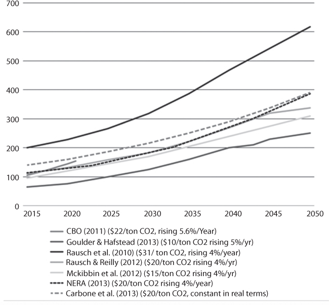
Figure 9.43 Projected gross revenue from a carbon tax (billions of $2012) (From Goulder and Hafstead, 2013).
The latest in this carbon tax saga has been the pandering of ‘double dividend’, which would convert the revenue from an environmental tax to boost economic activity or economic efficiency. The two “dividends” are: a reduction in pollution emissions; and a boost in GDP and/or economic efficiency from the use of the environmental tax revenue. Of course, this conclusion assumes that actual pollution reduction is carried out with carbon tax-related activities and in addition the tax money would actually be invested in boosting the economy. In fact these two premises are demonstrably false as discussed by Islam et al. (2018a).
Three categories of economic dividends are purported to exist. They are: 1) cuts in other taxes (such as payroll taxes or corporate or personal income taxes); 2) reducing the government budget deficit; and 3) financing valuable public spending.
The argument for why using carbon tax revenue to pay for cuts in other taxes boosts the economy is the same as the old ‘trickle down’ economics. Cutting corporate income taxes and personal income taxes on capital gains, dividends, and interest increases the incentive to save and invest, thus promoting capital accumulation. Cutting taxes on labor income is believed to have a similar effect by boosting incentives to work and to invest in human capital, thus increasing labor supply and labor force productivity. In either case, the result is an increase in the productive capacity of the economy, and thus a long-run boost in the level of economic activity. This also corresponds to a boost in economic efficiency, as those tax cuts reduce the tax distortions in labor and capital markets. All these, of course, assume corporations are benevolent and can be trusted to reinvest instead of hording the money. They also assume that humans, by their very nature, will be inspired to be more benevolent and above all the government can be trusted to be the caretaker of this process. Islam et al. (2018a) have detailed how the current pitiful state of the world is because of this paradoxical economic model.
Instead of addressing the paradoxes of this approach, Economic models suggest that the net effect of a carbon tax (with revenues used to cut labor/capital taxes) on the overall economy would be slightly negative, though much smaller than the effect of the carbon tax by itself. For example, Carbone et al. (2013) finds that imposing a carbon tax and using the revenue to fund cuts in taxes on labor still leads to a net reduction in GDP, but that the economic boost from the labor tax cuts offsets more than 80 percent of the effect of the carbon tax itself – so the net reduction in GDP is tiny. Consider the impact if the assumptions of benevolence and effectiveness are removed.
The paradoxical model is taken one step further. It is perpetrated that the tax cut could more than offset the effect of the carbon tax, and thus actually have a slight positive overall effect on GDP. For example, Parry and Williams (2010) take into account the effects of tax preferences – exemptions and deductions (like those for employer medical insurance and owner-occupied housing) that are large and pervasive across the US tax system. These deductions and exclusions narrow the base of income and other taxes, making them less efficient – and thus boosting the economic gain from cutting them. As a result, the net effect of the carbon tax shift can be to increase GDP. In reality, this scenario will never be reached unless there is a fundamental shift in government structure and its power over corporations (Islam et al., 2018).
The prospects for a net gain also depend on what other tax is cut. Most studies find that the biggest economic gains come from cutting taxes on capital, particularly from cutting the corporate income tax rate. Translation? The investment in non-human or mechanical assets will have the biggest impact on the society. In reality, the opposite occurs. Any investment in large infrastructure means more damage to the environment, more corporation profiteering, and more control of the government. The depiction in Figure 9.44 transforms the fallacious argument into a justification of imposing carbon tax. Figure 9.44 displays the estimated effects on the level of GDP resulting from the imposition of a carbon tax, for a total of seven different model runs taken from four different studies. This depiction actually shows that imposing a carbon tax and using the revenues to cut taxes on capital can yield a small net gain for the economy. For example, Carbone et al. (2013) finds that the net effect of a $30/ton carbon tax with the revenues used to cut taxes on capital is to increase GDP by about 1 percent in 20 years.

Figure 9.44 Projected impacts of carbon tax shifts on GDP (% change), selected results. (Goulder and Hafstead, 2013)
It is no surprise all these models show similar results although they emerge from apparently different premises. This is the case because they all start with the same set of false premises. This aspect is discussed latter in this section.
At this point, the discussion leads to what should be the upper limit of carbon tax. The NERA (2013) study (performed for the National Association of Manufacturers), which estimates that a carbon tax sufficient to reduce carbon emissions by 80 percent would cause GDP to be 3.4 percent lower in 2050 than it would have been without the carbon tax – a quite substantial drop. The reason this case is so different is that it represents a much higher carbon tax rate than any of the other studies: the carbon tax rate in that case is approximately $1,000 per ton by 2050 (which might be impractically high), whereas none of the other studies have a rate over $60/ton by 2050. The higher the carbon tax rate, the more substantial the effect on the economy, so it is not surprising that such an extremely high rate would have major effects on the economy. The conclusion, therefore, becomes carbon tax is effective as long as it is limited to a ‘decent’ number.
Often the budget deficit aspect of tax imposition relies on the example of the Great Recession, the outlook for medium- and long-run deficits are cause for concern (Gale and Harris, 2011). While the most recent projections from the Congressional Budget Office indicate that the deficit will shrink slightly over the next few years, those projections also indicate that the deficit and the debt-to-GDP ratio are set to rise substantially over the longer term. It is stated that large government budget deficits can retard economic growth in a variety of ways. Government borrowing creates additional demand in capital markets, thus potentially driving up interest rates and crowding out private investment. The need to eventually pay off the debt – or just to pay the interest on it – means that tax rates will need to rise in the future, cutting economic growth then (and perhaps also affecting the economy today, as workers and investors anticipate future tax increases). Also, a larger debt-to-GDP ratio increases the risk of a debt crisis.
Carbone et al. (2013) suggest that over the long term, the economic gain from using carbon tax revenues to reduce the deficit is generally substantially larger than the gain from using those revenues to cut taxes now. This result is driven primarily by the effects of higher future taxes: because the deficit is currently higher than a long-run sustainable level, future taxes will need to be higher than taxes today. The higher the tax rate, the more harmful a tax increase will be, so it is more efficient to raise additional revenue now (at today’s lower rates) than it will be later. The study does not fully capture the other effects of deficits (mentioned above), and thus likely understates the gains from deficit reduction. Carbone et al. (2013) also indicate one reason why addressing the budget deficit is so difficult: even though using carbon tax revenues to fund cuts in the deficit leads to substantially larger gains over the long term than using those revenues to fund tax cuts today, today’s voters tend to be better off with tax cuts today, whereas those who benefit more from deficit reductions are too young to vote (or not yet born). This analysis relies on the benevolence of the government as well as the corporation in general.
A third potential pro-growth use for carbon tax revenue would be to fund particularly valuable government spending. If the government has set the mix of taxes and spending efficiently, then the gains from funding an additional dollar of spending will equal the gains from a dollar of tax cuts. This is perhaps the most illogical argument in favour of carbon tax. History shows us at no time a government has grown to be more effective. Not a single government project in environmental remediation has yielded even decent result (Islam et al., 2018a).
The overwhelming conclusion of modern economic analysis is that a carbon tax could help mitigate future economic damage from climate change. However, a true scientific analysis by Islam et al. (2018a) shows the opposite.
An excellent manifestation of such outcome, supporting carbon tax, was captured in 2013, when the economist Robert J. Shiller shared the Nobel prize with Eugene Fama, while subscribing to two opposite view on the process of financial market (Applebaum, 2013). Similar to the above figures, it is perceived that any instability caused by either natural events or by government imposition would result in an eventual equilibrium, always settling with a positive outcome. Figure 9.45 shows how reality is trashed while promoting falsehood as the standard of the truth, thus creating a paradigm shift in the wrong direction.
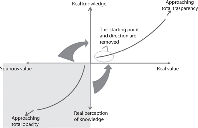
Figure 9.45 Falsehood is turned into truth and ensuing disinformation makes sure that truth does not come back in subsequent calculations. (From Islam et al., 2018)
Figure 9.46 shows how this deceptive process works. First, the connection between real values and real knowledge is removed. For economics, it would be removing the role of intention or conscience from the economic analysis. Then, spurious values are assigned to false perception of real knowledge. In this process, opacity is an asset and any process that can potentially reveal the opaque nature of the science of economics is shunned. Instead, mathematics that would glamourize the process of opacity is celebrated. In essence, the bottom left quadrant is brought to the right top quadrant and more the opacity more becomes the profit margin. Once this ‘fact’ is established, it becomes a matter of race to get to the most opaque solution and touting it as a progress, often branding it as a breakthrough discovery. This process of scientific disinformation amounts to taking the left quadrant with spurious values and turn it around to the top right quadrant, thereby promoting the implosive disastrous model as the ‘knowledge model’. The most stunning outcome of this process of mechanization is the robotization of humans. Metaphorically depicted in Picture 9.4, it involves false and illogical assertion continuous transition from ape to humans, essentially disconnecting conscience or the fundamental trait of humanity from humanity, then set robot or virtual reality as the ultimate model for humanity.
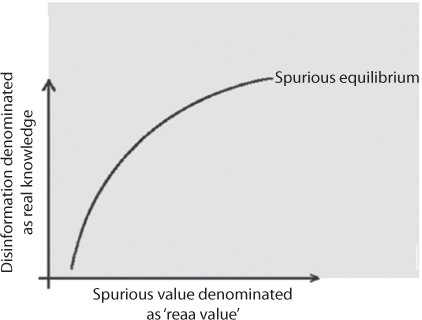
Figure 9.46 A new paradigm is invoked after denominating spurious value as real and disinformation into ‘real knowledge’.

Picture 9.4 Robotization is embedded into the fundamental assumptions.
What we see in the process is, all economists start off with the premise that carbon tax is good for the environment and the economy, then they revel by the finding that indeed their conclusions support their first premise.
9.9 Conclusions
The mindset of the economics model is deconstructed with regards to climate change. The fundamental assumptions behind major economic models used to justify control of policies related to climate are examined and tallied against facts related to greenhouse gases. It is shown that the economic models are the same that have been discredited from scientific perspective. The lack of real science behind climate change predictive models is exposed. Detailed deconstruction of Copenhagen and Paris Agreements are made. It is shown that both of them eventually had the hidden agenda of justifying carbon tax. Finally, the negative impacts of carbon tax are presented while refuting the incessant assertion of the mainstream economists and scientists that carbon tax is the only solution to the climate change crisis.