Chapter 10
The Science of Global Warming
10.1 Introduction
Global hydrological cycle is integral to the climate system. Even though it has become customary to present climate change as a distinct crisis, the overall climate change pattern depends on the entire ecosystem. In focus is the global temperature that shows a consistent upward slope in the modern era, synchronized with modern data collection techniques. Ever since the creation of The Intergovernmental Panel on Climate Change (IPCC) in 1988, numerous projects have been dedicated to collecting data as well as projection with various models (e.g., Figure 10.1). As discussed in previous chapters, these predictive models are rudimentary and do not have scientific basis.

Figure 10.1 IPCC FAR BAU global surfacetemperature projection adjusted to reflectobserved GHG radiative forcings 1990-2011 vs. observed surfacetemperature changes (average of NASA GISS, NOAA NCDC, and HadCRUT4) for 1990 through 2012 (Houghton et al., 2001).
However, the lack of scientific foundation did not stop scientists from making claims. Scores of publications have claimed to know the exact temperature from centuries (even millennia) of the history or to make predictions for centuries to come. They have often added contributions of human activities – meaning activities related to fossil fuel production and utilization Figure 10.2. For these as well, there has been no scientific rigor. For instance, none considered the long-term impact of the use of pesticide, chemical fertilizers, and genetic alteration on the quality of atmospheric health.

Figure 10.2 Evolution of global mean surface temperature (GMST) over the period ofinstrumental 24 observations. Grey line shows monthly mean GMST in the HadCRUT4, NOAA, GISTEMP and 25 Cowtan-Way datasets, expressed as departures from1850–1900, with line thickness indicating 26 inter–dataset range. Allobservational datasets shown represent GMST as a weighted average of 27 nearsurface air temperature over land and sea surface temperature over oceans.Human–induced 28 (yellow) and total (human– and naturally–forced, orange)contributions to these GMST changes (Houghton et al., 2001).
Numerous stations have been installed and they have generated volumes of data. In general, the bias in data collection has been attributed to the time of data collection and locations of the station (Williams et al. (2012). These two biases have been the focus of subsequent studies (Muller et al. 2012) and few, if any, have ventured into commenting on the applicability of the data, let alone scientific merit of the data collected. It is true, that considerable bias exists regarding stations’ predominant coverage of developed nations and very poor coverage of polar regions (Cowtan and Way, 2014). However, a scientific study that would actually question the parameters that are being monitored is what is lacking.
In this chapter, a scientific investigation is conducted in order to answer questions that have eluded previous researchers. The discussion identifies real source of global warming and unravels the mysteries surrounding climate change issues.
10.2 Current Status of Greenhouse
There is no doubt, there is almost 100% consensus that there is a climate change crisis that is caused by anthropogenic CO2 and is manifested through a rise in global temperature (Trivedi et al., 2013). In previous chapters, we have presented numerous graphs, depicting millennia of data, all allowing to ‘prove’ that that we are facing a great crisis that challenges the existence of the planet hearth. The reason that CO2 is a suspect is that CO2 is readily absorbed in the ocean that acts as a sink for virtually unlimited amount of CO2, yet the atmospheric concentration has been rising. In this analysis, CO2 has been lumped with other greenhouse gases, although unlike other greenhouse gases, CO2 is readily used by plants to synthesize carbohydrate, quickly renewing the life cycle. Compare that with, for instance, aerosols – the synthetic kind. Aerosols are not absorbed the environment and are instantly rejected by the ecosystem. Even methane and other greenhouse gases are subject to oxidation (at any temperature, because low-temperature oxidation is continuous). In addition, methane oxidation is a microbial metabolic process for energy generation and carbon assimilation from methane that is carried out by specific groups of bacteria, the methanotrophs. Methane (CH4) is oxidized with molecular oxygen to carbon dioxide, once again being reduced into useful gases. One can analyse each of the following greenhouse gases (listed in order of abundance) and show that there is no reason for them to become rejected by the ecosystem, except the last two, CFC, HCFC & HFC, which are not natural.
- Water vapour (H2O)
- Carbon dioxide (CO2)
- Methane (CH4)
- Nitrous oxide (N2O)
- Ozone (O3)
- Chlorofluorocarbons (CFCs)
- Hydrofluorocarbons (incl. HCFCs and HFCs)
As shown in Figure 10.3. the least amount released are the synthetic chemicals. Naturally, this depiction draws more attention to CO2.
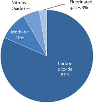
Figure 10.3 Greenhouse gasemission in 2016 (EPA, 2018).
Of course, in the bigger picture, CO2 is among trace gases, the concentration of all of which combined is less than 0.1%. The permanent gases whose percentages do not change from day to day are nitrogen, oxygen and argon. Nitrogen accounts for 78% of the atmosphere, oxygen 21% and argon 0.9%. Trace gases are: carbon dioxide, nitrous oxides, methane, and ozone. Of course, the entire atmosphere is embedded in water, the vapour form of which has a concentration ranging from 0–4%, depending on the location and time of the day. Within the trace gases, CO2 is the most abundant (93.497%), followed by Neon (4.675%), Helium (1.299%), Methane (0.442%), Nitrous Oxide (0.078%), and Ozone (0.010%). Note that each of these components can be natural origin or artificial origin. For instance, N2O can occur in nature and as such wouldn’t pose a threat to the environment. However, when N2O is emitted from a catalytic converter, it contains tiny fragments of the catalysts and other materials that didn’t exist in nature before. This makes the N20 distinctly different from the naturally occurring ones. Because, New Science doesn’t have a means of tracking source of material in the process of material characterization, pathway analysis of artificial chemicals as opposed to natural chemicals has eluded all modern scientists. Had there been a characterization based on natural and artificial sources of matter, a new scientifically accurate image would appear.
As has been stated numerous times in previous chapters, in addition to geological scale variation, CO2 concentrations show seasonal variations (annual cycles) that vary according to global location and altitude. Several processes contribute to carbon dioxide annual cycles: for example, uptake and release of carbon dioxide by terrestrial plants and the oceans, and the transport of carbon dioxide around the globe from source regions (the Northern Hemisphere is a net source of carbon dioxide, the Southern Hemisphere a net sink). In addition to the obvious seasonal variations and long-term trends in CO2 concentrations, there are also more subtle variations, which have been shown to correlate significantly with the regular El Niño-Southern Oscillation (ENSO) phenomenon and with major volcanic eruptions. These variations in carbon dioxide are small compared to the regular annual cycle, but can make a difference to the observed year-by-year increase in CO2. These are much more significant events than the burning of some 100 million barrels of oil. Carbon dioxide enters the atmosphere through burning fossil fuels (coal, natural gas, and oil), solid waste, trees and wood products, and also as a result of certain chemical reactions (e.g., manufacture of cement). On the other hand, CO2 is removed from the atmosphere when it is absorbed by plants as part of the biological carbon cycle. There would be perfect balance had it not been for certain fraction of CO2 that becomes contaminated and as such rejected by the plants as part of the carbon cycle. Carbon dioxide being the most important component of photosynthesis, the estimation of this lost CO2 is the greatest challenge in describing the global warming phenomenon.
It is noted that CO2 concentrations in the air were reasonably stable (typically quoted as 278 ppm) before industrialization. Since industrialisation (typically measured from the mid-18th century), CO2 concentrations have increased by about 30 per cent, thus prompting the current hysteria against carbon. However, it is not clear why petroleum products are targeted because the petroleum era is much more recent that the industrial era.
Similar to CO2, Methane concentrations in the air were reasonably stable before industrialization, typically quoted as 700 ppb. Since industrialisation, methane concentrations have increased by more than 150 per cent to present day values (~1790 ppb in 2009). In contrast with CO2, the rise in methane concentration is attributed to a variety of agricultural practices, such as rice and cattle farming, as well as from the transportation and mining of coal, the mining and reticulation of natural gas and oil, from livestock and other agricultural practices, by the decay of organic waste in municipal solid waste landfills, and from wetlands in response to global temperature increases. Methane concentrations show seasonal variations (annual cycles) that vary according to global location and altitude. The major processes that contribute to methane annual cycles are:
- release from wetlands, dependant on temperature and rainfall;
- destruction in the atmosphere by hydroxyl radicals;
- transport of methane around the globe from source regions (the Northern Hemisphere is a net source of methane, the Southern Hemisphere a net sink).
Similar to CO2, there are the more subtle inter-annual variations in methane, which have been shown to correlate with the regular ENSO phenomenon and with major volcanic eruptions. These variations in methane are small compared to the regular annual cycle.
The variation in methane concentration is, therefore, not considered to be the cause of global warming. It is also true that bulk of methane is not inherently toxic to the environment. Unlike CO2, most of methane available in the atmosphere is a result of direct discharge rather than a product of chemical/thermal reaction in presence of artificial chemicals or energy sources.
Nitrous oxide concentrations in the air were reasonably stable before industrialisation (in the timeframe of human existence), typically quoted as 270 ppb (parts per billion molar). Since industrialization, nitrous oxide concentrations have increased by about 20 per cent to present day values (~330 ppb in 2017). Figure 10.4 shows concentrations of nitrous oxide in the atmosphere from hundreds of thousands of years ago through 2015. The data come from a variety of historical ice core studies and recent air monitoring sites around the world. Each line represents a different data source as reported by EPA.
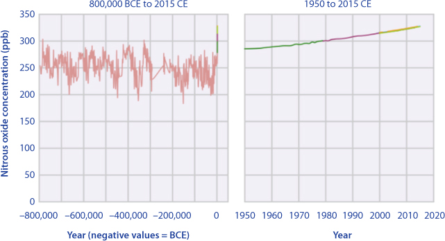
Figure 10.4 Nitrousoxide in the atmosphere (from EPA, 2018).
Nitrous oxide is a potent GHG with ~300-fold greater warming potential than CO2 on a per molecule basis, and is involved in destruction of the stratospheric ozone layer (Ravishankara et al., 2009). Globally, soil ecosystems constitute the largest source of N2O emissions (estimated at 6.8 Tg N2O-N/year), comprising approximately 65% of the total N2O emitted into the atmosphere, with 4.2 Tg N2O-N/year derived from nitrogen fertilization and indirect emissions, 2.1 Tg N2O-N/year arising from manure management and 0.5 Tg N2O-N/year introduced through biomass burning (IPCC, 2007). Other important N2O sources include ocean, estuaries and freshwater habitats and wastewater treatment plants (Schreiber et al. 2012). In recent years, the excessive use of nitrogen-based fertilizers (ca. 140 Tg N/year), has greatly contributed to the conspicuous elevation in atmospheric N2O concentrations, from pre-industrial levels of 270 ppbv. Generally, for every 1000 kg of applied nitrogen fertilizers, it is estimated that around 10–50 kg of nitrogen will be lost as N2O from soil, and the amounts of N2O emissions increase exponentially relative to the increasing nitrogen inputs (Shcherbak et al., 2014). Industrial activities, as well as during combustion of fossil fuels and solid waste are believed to be the cause of monotonous increase in Nitrous oxide.
Figure 10.5 shows different pathways that can generate NO2. The quality of NO2 will depend on the pathway travelled by various components. Hu et al. (2015) presented details of various techniques that can track the pathways. Even though this work can shed light on truly scientific characterization of matter, they do not identify a technique that would separate natural origin from the artificial (synthetic) one. For instance, their analysis doesn’t differentiate between chemical fertilizer and organic fertilizer. With the advent of new analytical tools, it is becoming possible to characterize matter with proper signatures (Wielderhold, 2015). Most recent developed will be discussed in a latter section.
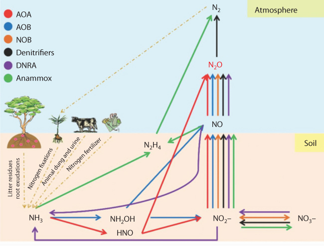
Figure 10.5 Simplifiedschematic representations of the major microbial pathways and microbes for theglobal N2O production and nitrogen cycling in soil ecosystems (FromHu et al., 2015) AOA: ammonia-oxidizing archaea; AOB: ammonia-oxidizingbacteria; NOB: nitrite oxidation; DNRA: dissimilatorynitrate reduction to ammonium; Annamox: anaerobic ammonium oxidation.
Hydrofluorocarbons, perfluorocarbons, sulfur hexafluoride, and nitrogen trifluo-ride are synthetic, powerful greenhouse gases that are emitted from a variety of industrial processes. Fluorinated gases are sometimes used as substitutes for stratospheric ozone-depleting substances (e.g., chlorofluorocarbons, hydrochlorofluorocarbons, and halons). These gases are typically emitted in smaller quantities, but because they are potent greenhouse gases, they are sometimes referred to as High Global Warming Potential (GWP) gases. GWP was developed in order to allow comparison of various greenhouses gases through their impact on global warming. The base is CO2 and other gases are measured relative to CO2. It is a measure of how much energy the emissions of 1 ton of a gas will absorb over a given period of time, relative to the emissions of 1 ton of carbon dioxide (CO2). The larger the GWP, the more that a given gas warms the Earth compared to CO2 over that time period. The time period usually used for GWPs is 100 years. By definition, CO2 has a GWP of 1 regardless of the time period used. Methane (CH4) is estimated to have a GWP of 28–36 over 100 years. Methane emitted today lasts about a decade on average, which is much less time than CO2. However, methane also absorbs much more energy than CO2. The net effect of the shorter lifetime and higher energy absorption is reflected in the GWP. Nitrous Oxide (N2O) has a GWP 265–298 times that of CO2 for a 100 year timescale. N2O emitted today remains in the atmosphere for more than 100 years, on average. Chlorofluorocarbons (CFCs), hydrofluorocarbons (HFCs), hydrochlorofluorocarbons (HCFCs), perfluorocarbons (PFCs), and sulfur hexafluoride (SF6) are sometimes called high-GWP gases because, for a given amount of mass, they trap substantially more heat than CO2. This characterization is useful but not entirely scientific as it doesn’t distinguish the composition of artificial chemicals within a gaseous system.
Although not considered before, clues to the answer of key climate change questions lie within monitoring the concentration of Chlorofluorocarbons (CFCs) in the atmosphere. These chemicals all had 0 concentration before the onset of the so-called plastic era, which saw mass production of artificial chemicals for ubiquitous applications. Figure 10.6 shows CFC concentrations as monitored by NORA (2018). The dashed marks are estimated values. NOAA monitors atmospheric concentrations of these chemicals and other important halocarbons at twelve sampling sites using either continuous instruments or discrete flask samples.
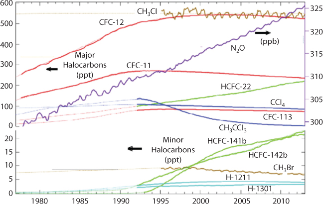
Figure 10.6 CFC concentration in atmosphere as monitored by NORA (2018).
Refrigerators in the late 1800s and early 1900s used the toxic gases, ammonia (NH3), methyl chloride (CH3Cl), or sulfur dioxide (SO2), as refrigerants. After a series of fatal accidents in the 1920s when methyl chloride leaked out of refrigerators, a search for a less toxic replacement began as a collaborative effort of three American corporations- Frigidaire, General Motors, and Du Pont. CFCs were first synthesized in 1928 by Thomas Midgley, Jr. of General Motors as safer chemicals for refrigerators used in large commercial applications. In 1932 the Carrier Engineering Corporation used FreonTM-11 (CFC-11) in the world’s first self-contained home airconditioning unit, called the “Atmospheric Cabinet”. During the late 1950s and early 1960s the CFCs made possible an inexpensive solution for air conditioning in many automobiles (CFC-12), homes, and office buildings. Later, the growth in CFC use took off worldwide with peak, annual sales of about a billion dollars (U.S.) and more than one million metric tons of CFCs produced. During the same time (1930), Einstein patented a technology for the same purpose that used ammonia, butane – a remarkable feat considering it used no electricity, had no moving part, and could operate without any synthetic chemical (Khan and Islam, 2012). While, this technology is making a comeback (Zyga, 2008), the science behind this technology and its merit in creating an engineering design without resorting to synthetic chemicals didn’t appeal to anyone for almost a century.
Instead, CFCs were promoted as ‘safe’ to use in most applications and ‘inert’ in the lower atmosphere. In 1974, two University of California chemists, Professor F. Sherwood Rowland and Dr. Mario Molina, showed that CFCs could be a major source of inorganic chlorine in the stratosphere following their photolytic decomposition by ultra-violet (UV) radiation there. Some of the released chlorine would become active in destroying ozone in the stratosphere. Ozone is a trace gas located primarily in the stratosphere. While this damage to the environment was recognized when “Ozone Holes” were discovered in 1980s and the synergistic reactions of chlorine and bromine and their roles recognized, the solutions offered was to reduce the production of these chemicals. For instance, in Montreal Protocol (on September 16, 1987), 27 nations signed a global environmental treaty to Reduce Substances that Deplete the Ozone Layer that had a provision to reduce production levels of these compounds by 50% relative to 1986 before the year 2000. This international agreement included restrictions on production of CFC-11,-12, -113,-114, -115, and the Halons (chemicals used as a fire extinguishing agents). An amendment approved in London in 1990 was more forceful and called for the elimination of CFC production by the year 2000. The chlorinated solvents, methyl chloroform (CH3CCl3), and carbon tetrachloride (CCl4) were added to the London Amendment as controlled substances in 1992. Subsequent amendments added methyl bromide (with exemptions for specific uses), hydrobromofluorocarbons, and bromochloromethane. This explains the peaks reached in various CFC graphs in Figure 10.6. So, how was the reduction of these chemicals compensated? Instead of finding chemicals that wouldn’t cause the kind of harm CFC was causing, other chemicals were produced that would delay the response of the environment although in long-term effects they were not any less desirable than CFC. For instance, two classes of halocarbon substituted for others. These are: hydrochlorofluorocarbons (HCFCs) and the hydrofluorocarbons (HFCs). The HCFCs include hydrogen atoms in addition to chlorine, fluorine, and carbon atoms. The advantage of using HCFCs is that the hydrogen reacts with tropospheric hydroxyl (OH), resulting in a shorter atmospheric lifetime. HCFC-22 (CHClF2) has an atmospheric lifetime of about 12 years compared to 100 years for CFC-12. This, however, says nothing about the fact that HCFC-22 is not compatible with the ecosystem. In fact, it is US EPA site that lists it as a candidate for high-temperature oxidation in order to mitigate (EPA, 2014). There lies another layer of disinformation. It is assumed that HCFC-22, a synthetic chemical that never existed in nature can be combusted into generating CO2 – a natural chemical that is essence of life on Earth.
EPA (2014) reports Global abatement potential in the HCFC-22 production sector is 228 million metric tons of carbon dioxide equivalent (MtCO2e) and 255 MtCO2e in 2020 and 2030, respectively, which equates to a 90% reduction from projected baseline emissions (Figure 10.7). It is then stated that thermal oxidation is the only abatement option considered for the HCFC-22 production sector, for a price tag of $one per tCO2. Then comes the solution in terms of tagging cleanup with increasing price Figure 10.8. We’ll see in latter section of this chapter that New Science is incapable of properly analyzing the real damage caused by these synthetic chemicals.
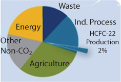
Figure 10.7 FluorinatedGreenhouse Gas Emissions from HCFC-22 Production (from EPA, 2014).
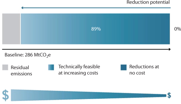
Figure 10.8 It would be cost-effective to reduce emissions by 0%, compared to the baseline, in 2030. An additional 89% reduction is available using technologies with increasingly higher costs (From EPA, 2014).
Curiously, New Science didn’t stop at avoiding artificial/natural sourcing, it used the presence of artificial sources to explain the paradoxical nature of CO2 cause effect narration. For instance, the warming this century occurred mostly between 1910 and 1940, when the carbon dioxide concentration grew slowly from 293 to 300 ppm. Meanwhile, the temperature remained steady between 1940–1980, while the carbon dioxide concentration increased from 300 to 335 ppm. These seemingly paradoxical behaviors are explained by the presence of atmospheric aerosol – the artificial variety ones. Aerosols are emitted by industrial processes, transport, etc, and their increased concentration offset simultaneous warming due to increasing greenhouse gases. However the warming overtook the cooling by mid 1970’s (Keeling et al., 1996).
Figure 10.9 Shows the latest details of greenhouse gas emissions in USA. Note that the only nitrous oxide and fluorinated gas show continuous increase, whereas carbon dioxide and methane show fluctuations over time.
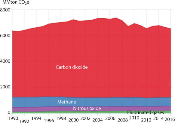
Figure 10.9 Nitrousoxide in the atmosphere (from EPA, 2018).
Figure 10.10 shows distribution of greenhouse gas among various sectors. As we’ll see in latter sections, CO2 generated from transportation, electricity generation, and industry are 100% contaminated and cannot be absorbed by the ecosystem. When it comes to agriculture, the production of contaminated CO2 is proportional to the practices of the region. For instance, in the west, beef is the most CO2-intesive operation. Gerber et al. (2013) give a complete details of greenhouse gases emitted from livestocks. For this sector, global emissions from the production, processing and transport of feed account for about 45 percent whereas fertilization of feed crops and deposition of manure on pastures generate substantial amounts of N2O emissions, representing together about half of feed emissions (i.e., one-quarter of the sector’s overall emissions). About one-quarter of feed emissions (less than 10 percent of sector emissions) are related to land-use change.

Figure 10.10 Distribution of greenhouse gas among various sectors in USA (EPA, 2017).
Among feed materials, grass and other fresh roughages account for about half of the emissions, mostly from manure deposition on pasture and land-use change. Crops produced for feed account for an additional quarter of emissions, and all other feed materials (crop by-products, crop residues, fish meal and supplements) for the remaining quarter. Enteric fermentation is the second largest source of emissions, contributing about 40 percent to total emissions. Cattle emit 77% of enteric CH4, buffalos 13%, whereas small ruminants emit about 10%. Methane and N2O emissions from manure storage and processing represent about 10 percent of this sector’s emissions. When energy consumption is tallied up, the total emissions amount to about 20%. This is the part that depends heavily on the region where the livestock is grown.
Today, this entire analysis doesn’t distinguish between organic or mechanical processes. For instance, methane emitted from enteric fermentation is lumped together with industrial methane from oil and gas activities, both being branded as ‘antropogenic methane’. Whereas, this enteric methane accounts for as much as 30% of global anthropogenic methane emissions.
The problem is very similar for N2O emission as well. In natural processes (including bacterial activities), N2O is integral part of vital functioning of NO (Wang et al., 2004). Whereas, NO2 emitted from industrial processes is inherently toxic to the environment and gets rejected by the ecosystem.
10.3 The Current Focus
At present all theories are geared toward targeting carbon as the source of global warming. In this process, CO2 is the paradigm and other gases are expressed as a CO2 equivalent. No distinction is made between organic CO2 (either naturally occurring or through biological process) and mechanical CO2 (generated through modern engineering).
10.3.1 Effect of Metals
Dupuy and Douay (2001) studied of the behavior of heavy metals in soils requires the knowledge of the complexation between soil constituents and metals and this information is not available from conventional analytical techniques such as atomic absorption. Since metals do not absorb mid infrared radiation, we wanted to characterize them using their interaction with the organic matter of soils. The use of chemometrics treatment of the spectroscopic data has demonstrated firstly that the interaction between soil constituents and metals takes place preferentially via organic matter, secondly the high difference between the complexation of lead and zinc into organic matter should be noted. The study of the infrared spectra shows that two bands at 1670–1690 and 1710 cm−1 vary according to the concentration of lead, which seems to be preferentially complexed by the salicylate functionality.
Five distinct layers have been identified based on following features (NOAA, 2018)
- thermal characteristics (temperature changes);
- chemical composition;
- movement; and
- density.
Each of the layers are bounded by “pauses” where the greatest changes in thermal characteristics, chemical composition, movement, and density occur. These five basic layers of the atmosphere are Figure 10.11:
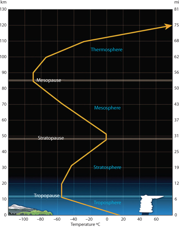
Figure 10.11 Various atmosphericlayers and their principal features (from NOAA, 2018a).
Exosphere: This is the outermost layer of the atmosphere and is external to our atmospheric system. It extends from the top of the thermosphere to 10,000 km above the earth. In this layer, all matters escape into space and satellites orbit the earth. At the bottom of the exosphere is the thermopause located around 375 miles (600 km) above the earth.
Thermosphere: This layer is between 85 km and 600 km from the surface of the earth. This layer is known as the upper atmosphere. The density of gases is very low but starts to increase drastically toward lower layers. In this layer that high energy ultraviolet and x-ray radiation from the sun begins to be absorbed by the molecules in this layer, causing temperature increases. Because of this absorption, the temperature increases with height. From as low as –120 C at the bottom of this layer, temperatures can reach as high as 2,000 C near the top. However, even at that high temperature, the actual heat retention is not large because of the low density of matter in that layer.
Mesosphere: This layer extends from around 50 km above the Earth’s surface to 85 km. In this layer, the density of gases increases drastically, accompanied with rise in ambient temperature. This is the layer that is dense enough to slow down meteors hurtling into the atmosphere, where they burn up, leaving fiery trails in the night sky. The transition boundary which separates the mesosphere from the stratosphere (next one) is called the stratopause.
Stratosphere: The Stratosphere extends around 50 km down to anywhere from 6 to 20 km above the surface of the Earth. This layer holds 19 percent of the atmosphere’s gases but very little water vapor. In this region the temperature increases with height. Heat is produced in the process of the formation of Ozone and this heat is responsible for temperature increases from an average –51 C at tropopause to a maximum of about –15 C at the top of the stratosphere. As such, warmer air is located above the cooler air, thus minimizing intra-layer convection.
Troposphere: The troposphere begins at the surface of the Earth and extends from 6 to 20 km high. The height of the troposphere varies from the equator to the poles. At the equator it is around 18–20 km high, at 50°N and 50°S, 85 km and at the poles just under 65 km high. The sun’s rays provide both light and heat to Earth, and regions that receive greater exposure warm to a greater extent. This is particularly true of the tropics, which experience less seasonal variation in incident sunlight. As the density of the gases in this layer decrease with height, the air becomes thinner. Therefore, the temperature in the troposphere also decreases with height in response. As one climbs higher, the temperature drops from an average around 17 C to –51 C at the tropopause.
Scientists have spent great amount of time and energy in explaining how greenhouse gases have created the global warming. At present, it is theorized that many molecules in the atmosphere possess pure-rotation or vibration-rotation spectra that allow them to emit and absorb thermal infrared (IR) radiation (4–100 μm), such gases include water vapor, carbon dioxide and ozone (but not the main constituents of the atmosphere, oxygen or nitrogen). It is this property that gives special status for greenhouse gases. Because this absorption of IR prevents heat from escaping the earth, the greenhouse gas effect kicks in. It is customary to consider that convection is the dominant mechanism below tropopause. As such, it is often justified that instant mixing occurs up to that interface. Overall, thermal balance is maintained through exchange of IR back and forth from the Earth’s surface. Consequently, the change in the radiative flux at the triopopause, which marks the interface between convective layer and a stable layer becomes the most crucial zone for overall climate control (Ramanathan et al., 1987). Mechanically, Earth’s spin creates three belts of circulation due to its continuous spinning motion (Stevens, 2011). Air circulates from the tropics to regions approximately 30° north and south latitude, where the air masses sink. This belt of air circulation is referred to as a Hadley cell, after George Hadley, who first described it (Holton, 2004). Two additional belts of circulating air exist in the temperate latitudes (between 30° and 60° latitude) and near the poles (between 60° and 90° latitude). A further consideration is the spectroscopic strength of the bands of molecules which dictates the strength of the infra-red absorption. Molecules such as the halocarbons have bands with intensities about an order of magnitude or greater, on a moleculeper-molecule basis, than the 15 |im band of carbon dioxide. This is further impacted by the presence of any fraction of artificial chemicals that often have heavy metals. The actual absorbance by a band is, however, a complicated function of both absorber amount and spectroscopic strength so that these factors cannot be considered entirely in isolation.
Other factors involve radiative forcing and in particular the spectral absorption of the molecule in relation to the spectral distribution of radiation emitted by a matter. The distribution of emitted radiation with wavelength is shown by the dashed curves for a range of atmospheric temperatures as shown in Figure 10.12. Unless a molecule possesses strong absorption bands in the wavelength region of significant emission, it can have little effect on the net radiation. The solid line shows the net flux at the tropopause (Wm2) in each 10 cm-1 interval using a standard narrow band radiation scheme and a clear-sky mid-latitude summer atmosphere with a surface temperature of 294K (Shine et al., 1990). Under this scenario, the wavelength is important.

Figure 10.12 Spectrum of variousemissions from a black body (Wm2 per 10 cm−1 spectral interval) across the thermal infrared for temperatures of 294K, 244K and 194K (from Shine et al., 1990).
There has been a perfect balance in the concentration of naturally occurring gases in the atmosphere and all strata that are described above. These concentrations dictate the level of absorption that would take place within the tropopause. It is understood that gases, such as halocarbons that didn’t exist in nature before, the forcing is linearly proportional to the concentration. On the other hand, for gases such as methane and nitrous oxide, their forcings are considered to be proportional to the square root of their concentration (Shine et al., 1990). For CO2, the spectrum is so opaque that additional molecules of carbon dioxide are considered to have little impact, making forcing to be logarithmic in concentration. Molecules such as the halocarbons have bands with intensities about an order of magnitude or even greater, on a molecule-per-molecule basis, than the 15 μm band of carbon dioxide The actual absorptance by a band is, however, a complicated function of both absorber amount and spectroscopic strength so that these factors cannot be considered entirely in isolation (Rey et al., 2018). Initial work of Rey et al. (2018) indicates that for these artificial chemicals (CF4 in this particular case), “hot bands” corresponding to transitions among excited rovibrational states contribute significantly to the opacity in the infrared even at room temperature conditions. Such molecules have a particularly long atmospheric lifetime (scientifically, they never become assimilated with the ecosystem) and their very estimated global warming potentials are very large. They report a list on such data for CF4 in the range 0–4000 cm−1, containing rovibrational bands that are the most active in absorption. is partitioned into strong & medium intensity transitions and the quasi-continuum of individually indistinguishable weak lines. The latter ones are compressed using “super-lines” (SL) databases for an efficient modelling of absorption cross-sections (Figure 10.13).
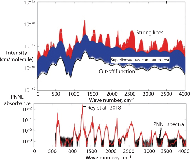
Figure 10.13 Top panel: Strong lineintensities (in red) and schematic representation of the quasi-continuum area(QC, in blue, treated using super-lines) of tetrafluoromethane at296 K. A plot of the cutoff function is also given (black line). Bottom panel:Plot of the PNNL absorbance and comparison with TheoReTS (From Rey et al., 2018).
This behavior is strongly affected by the presence of heavy metals (Vernooij et al., 2016). Table 10.1. gives atomic absorption data for select metals, along with their intensity and corresponding wave numbers.
Table 10.1 Atomic absorption data for certain elements (From Sansonettia and Martin, 2005).
| Element | Ground state | Ionization energy | Intensity/wavelength (air) |
| Pb I | 1s22s22p63s23p63d104s24p64d104f145s25p65d106s2 6p21/2(1/2,1/2)0 | 59819.2 cm−1(7.411663 eV) | 90/2663.154 |
| Pb II | 1s22s22p63s23p63d104s24p64d104f145s25p65d106s2 6 p2P01/2 | 121 245.14 cm−1(15.03248 eV) | 50/3713.982 |
| Hg I | 1s22s22p63s23p63d104s24p64d104f145s25p65d106s21S0 | 84184.1 cm−1(10.4375 eV) | 80/3131.839 |
| Hg II | 1s22s22p63s23p63d104s24p64d104f145s25p65d106s2S1/2 | 151284.4 cm−1(18.7568 eV) | 60/2260.294 |
| Pt I | 1s22s22p63s23p63d104s24p64d104f145s25p65d96s3D3 | 72257.3 cm−1(8.9588 eV) | 30/1971.5374 |
| Pt II | 1s22s22p63s23p63d104s24p64d104f145s25p65d92D5/2 | 149723 cm−1(18.563 eV) | 30/1954.7436 |
| Cd I | 1s22s22p63s23p63d104s24p64d105s21S0 | 136374.74 cm−1(16.908 31 eV) | 150/3252.524 |
| Cd II | 1s22s22p63s23p63d104s24p64d105s2S1/2 | 136374.74 cm−1(16.908 31 eV) | 200/2321.074 |
| Cu I | 1s22s22p63s23p63d104s2S1/2 | 62317.44 cm−1(7.72638 eV) | 150P/2178.94 |
| Cu II | 1s22s22p63s23p63d104s1S0 | 163669.2 cm−1(20.2924 eV) | 150P/1999.698 |
| Fe I | 1s22s22p63s23p63p63d64s25D4 | 63737 cm−1(7.9024 eV) | 40/2373.6245 |
| Fe II | 1s22s22p63s23p63p63d64s6D9/2 | 63737 cm−1(7.9024 eV) | 40/2363.8612 |
10.3.2 Indirect Effects
In addition to their direct radiative effects, many of the greenhouse gases also have indirect radiative effects on climate through their interactions with atmospheric chemical processes. Note that these processes are continuous and take place under any temperature and pressure, albeit at different rates. In addition, the presence of contaminats alter the nature of these reactions, as will be shown in latter section of this chapter. Some of these interactions are listed in Table 10.2.
Table 10.2 Direct radiative effects and indirect trace gas chemical-climate Interactions (Shine et al. 1990).
| Gas | Greenhouse gas? | Is its tropospheric concentration affected by chemistry | Effects on tropospheric chemistry? | Effects on stratospheric chemistry? |
| CO2 | Yes | No | No | Yes, affects O3 |
| CH4 | Yes | Yes, reacts with OH | Yes, affects OH, O3 and CO2 | Yes, affects O3 and H2O |
| CO | Yes, but weak | Yes, reacts with OH | Yes, affects OH, O3 and CO2 | Not significantly |
| N2O | Yes | No | No | Yes, affects O3 |
| NOX | Yes | Yes, reacts with OH | Yes, affects OH and O3 | Yes, affects O3 |
| CFC-11 | Yes | No | No | Yes, affects O3 |
| CFC-12 | Yes | No | No | Yes, affects O3 |
| CFC-113 | Yes | No | No | Yes, affects O3 |
| HCFC-22 | Yes | Yes, reacts with OH | No | Yes, affects O3 |
| CH3Cl3 | Yes | Yes, reacts with OH | No | Yes, affects O3 |
| Cl2CFBr | Yes | Yes, reacts with OH | No | Yes, affects O3 |
| CF3Br | Yes | No | Yes, affects O3 | |
| Yes, but weak | Yes, reacts with OH | Yes, increases aerosols | Yes, increases aerosols | |
| cs3scs3 | Yes, but weak | Yes, reacts with OH | Source of SO2 | Not significantly |
| CS2 | Yes, reacts with OH | Source of COS | Yes, increases aerosols | |
| COS | Yes but weak | Yes, reacts with OH | Not significant | Yes increases with aerosol |
| O3 | yes | yes | yes | yes |
This table focuses on the role of Ozone. Ozone plays an important dual role in affecting the climate. Ozone concentration in the atmosphere depends on its vertical distribution throughout troposphere and stratosphere. This is in addition to concentration in the atmosphere – this concentration being dynamic as Ozone concentration is not stable like other greenhouse gases, such as CO2. Ozone is also a primary absorber of solar radiation in the stratosphere, thus contributing to the increase with altitude. The greenhouse effect is directly proportional to the temperature contrast between the level of emission and the levels at which radiation is absorbed. This contrast is greatest near the tropopause, where temperatures are at a minimum compared to the surface. Above about 30 km, added ozone causes a decrease in surface temperature because it absorbs extra solar radiation, effectively depriving the troposphere of direct solar energy that would otherwise warm the surface (Lacis et al, 1990). Lacis et al. (1990) observed a cooling of the surface temperature at northern mid-latitudes during the 1970s equal in magnitude to about half the warming predicted for CO2 for the same time period. However, the measurement uncertainty of the observed trends is large, with the best estimates for mid-latitude cooling being –0.05 ± 0.05 °C. The surface cooling was determined to be caused by ozone decreases in the lower stratosphere, which outweigh the warming effects of ozone increases in the troposphere. The results obtained differ from predictions based on one-dimensional photochemical model simulations of ozone trends for the 1970s, which suggest a warming of the surface temperature equal to ~20% of the warming contributed by CO2. Also, the ozone decreases observed in the lower stratosphere during the 1970 s produce atmospheric cooling by several tenths of a degree in the 12- to 20-km altitude region over the northern mid-latitudes. This temperature decrease is larger than the cooling due to CO2 and thus may obscure the expected stratospheric CO2 greenhouse signature.
The presence of metals affect the IR absorption. This principle has been used for material characterization, the technique being called Surface-enhanced IR absorption (SEIRA). It is established that IR absorption of molecules adsorbed on metal nanoparticles is significantly enhanced than would be expected in the normal measurements without the metal (Miki et al., 2002). SEIRA spectroscopy (SEIRAS) has been applied to in situ study of electrochemical interfaces. A theoretical calculation predicts that SEIRA effect can be observed on most metals if the size and shape of particles and their proximity to each other are well tuned. It has been observed for Au, Ag, Cu, and Pt. From a comparison with the spectra of CO adsorbed on smooth Pt surfaces, it has been reported that the absorption is 10–20 times enhanced on Pt nanoparticles (Miki et al., 2002).
Figure 10.14 shows the fluxes of energy in and out of Earth’s surface. The Sun provides most of the incoming energy, shown in yellow. Most of this energy is absorbed at the surface with the exceptions of:
- - energy reflected by clouds or the ground; and
- - energy absorbed by the atmosphere.
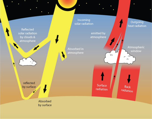
Figure 10.14 Overall energy balanceof the Earth (From NASA, as reported in Rosen and Egger, 2016).
Most of the outgoing energy is emitted by Earth’s surface as long wavelength radiation, shown in red in Figure 10.14. These are the radiations that mostly get absorbed by greenhouse gases the atmosphere. The atmosphere re-emits some of this energy up to space and some of it back down to Earth. The red arrow labeled “back radiation” represents the greenhouse effect, which can create imbalance if there is a perturbation in thermochemical features of the atmosphere.
Arrhenius set out to account for all the energy coming into and leaving the Earth system – a kind of energy budget (Arrhenius, 1896). That required tallying up all the sources of energy, the ways energy could be lost (known as energy sinks) and the ways energy could be transferred (known as energy fluxes). Arrhenius did not include an illustration in his 1896 paper, but essentially captured what is shown in Figure 10.14. This diagram shows the fluxes of energy in and out of Earth’s surface. The Sun provides most of the incoming energy, shown in yellow. Most of this energy is absorbed at the surface, except for a small amount that gets reflected by clouds or the ground, or that gets absorbed by the atmosphere. Most of the outgoing energy is emitted by Earth’s surface as long wavelength radiation, shown in red. However, most of this energy gets absorbed by greenhouse gases in the atmosphere. The atmosphere re-emits some of this energy up to space and some of it back down to Earth. The red arrow labeled “back radiation” represents the greenhouse effect. Thin black arrows in Figure 10.14 represent solar radiation in Arrhenius’ equation. Because long-wave infrared radiation is absorbed by greenhouse gases, they were known to have a role in global temperatre.
Arrhenius reasoned that if the atmosphere was absorbing infrared radiation, it too was heating up. Thus, he added another level of complexity to his model: an atmosphere that could absorb and radiate heat just like Earth’s surface. For simplicity, he treated the whole atmosphere as one layer. The atmosphere absorbed outgoing radiation emitted by the surface (thick red arrow), and then emitted its own radiation both up to space and back down to Earth (thin red arrows). This was the beginning of the so-called 2-layer model.
This was an important realization, because it showed that the atmosphere didn’t block outgoing radiation as Fourier had proposed. It absorbed it. Then, like the hotbox, it heated up and emitted infrared energy. The atmosphere emits this energy in all directions, including back toward the earth. This flux of energy from the atmosphere to the surface represents another important source of heat to Earth’s surface, and it explains the real mechanism behind the greenhouse effect.
10.4 Scientific Characterization of Greenhouse Gases
It has been known for some time that biogeochemical cycling of anthropogenic metals can attach an isotopic signature during the biological processing in a natural environment. If this signature is often accompanied by stable isotope fractionation, which can now be measured due to recent analytical advances (Wiederhold, 2015). A new research field involves complementing the traditional stable isotope systems (H, C, O, N, S) with many more elements across the periodic table (Li, B, Mg, Si, Cl, Ca, Ti, V, Cr, Fe, Ni, Cu, Zn, Ge, Se, Br, Sr, Mo, Ag, Cd, Sn, Sb, Te, Ba, W, Pt, Hg, Tl, U), which then can be potentially applied as novel geochemical tracers. The same technique can also shed light on the application of metal stable isotopes as source and process tracers in environmental studies. Wiederhold (2015) introduced most important concepts of mass-dependent and mass-independent metal stable isotope fractionation and their effects on natural isotopic variations (redox transformations, complexation, sorption, precipitation, dissolution, evaporation, diffusion, biological cycling, etc.).
It is known that stable isotope ratios of chemical elements in environmental samples contain valuable information on sources and processes that elements were exposed to, in essence carrying the signature of the pathway all the way going back to the source. For decades, there has been a flux of new techniques for isotope analysis of light elements (H, C, O, N, S) and their applications to environmental geochemistry (Hoefs, 2009; Fry, 2006). These stable isotope systems encompass only elements, which can then be converted into a gaseous form, thus being amenable to gas-source mass spectrometers (de Groot, 2008). For decades, the main difficulty in analysis techniques was the lack of technique suitable for discerning natural variations in the stable isotope composition of heavier elements, especially metals. This capability has been enhanced greatly over last few years, during which period the high-precision stable isotope analysis techniques have been expanded to almost the entire periodic table. This includes primarily the present-day cycling of metals and metalloids in the environment related to their important roles as:
- integral components of earth surface processes (e.g., weathering, pedogenesis);
- as nutrients for organisms (e.g., plants, microorganisms); and
- as pollutants affecting natural ecosystems as a result of anthropogenic activities (e.g., emissions from industrial or mining sources).
10.4.1 Connection to Subatomic Energy
Islam (2014) presented comprehensive mass-energy balance equation that erases the artificial boundary between mass and energy. Every chemical reaction involes mass transfer and every mass transfer involves energy transfer. Starting with Newton, mass and energy have been disconnected in all analyses of New Science. Only recently, it has been recognized that energy exchange is inherent to chemical reactions1. Problem, however, persists because currently there is no mechanism to discern between organic/natural mass and synthetic/artificial mass, which are the source of organic energy and artificial energy, respectively. The use of quantum chemistry has made the situation worse because instead of seeking scientific reasoning, it has made it easier to invoke dogmatic and often paradoxical concepts. Even then, the latest discoveries are useful in gaining insight into physic-chemical reactions. In that regard, Rahm and Hoffmann (2015) introduced new ways of understanding the origins of energy in chemical reactions Starting with the premise that all of the interactions between the molecules, atoms, and the electrons that bind atoms together can collectively be understood in terms of energy, they propose a new energy decomposition analysis in which the total changing energy of any chemical reaction can be broken down into three components:
- nuclear-nuclear repulsion (the repulsive energy between the positively charged nuclei of different atoms);
- the average electron binding energy (the average energy required to remove one electron from an atom); and
- electron-electron interactions (the repulsive energy between negatively charged electrons).
The first one (repulsion) occurs when two atoms are brought together by decreasing the distance between nuclei. This repulsion leads to accumulation of electron to fill in the space caused by repulsion. In the presence of the two nuclei, the average binding energy of the electrons changes due to differences in electron-nuclear attraction. As the electrons move closer together, they also begin to interact more strongly with each other. At this point, quantum chemistry focuses on quantifying these electron-electron interactions with the assumption that all electrons are similar, irrespective of what element it belongs to. We argued in previous chapters that not only they are different from element to element, they are also different in their spinning depending on the source of the element, meaning a natural source would have them spin in a different direction from the direction of artificial sources. Not surprisingly, Rahm and Hoffmann (2015) focused on the electron interactions and estimated their interactions from experimental data, relying on quantum analysis. Conventionally a wave function is used to estimate the solutions to the Schrödinger equation, which assumes simultaneous existence of the wave–particle duality. They used experimental data to correlate with solutions of quantum equations to justify their applicability. Similarly, electronegativity, an old term used to describe is propensity of an atom to attract a bonding pair of electrons, was redefined. When Nobel laureate Chemist, Linus Pauling first defined this term in 1932, he referred to it as “the power of an atom to attract electrons to itself.” An alternative definition was proposed by Allen (1989), who introduced electronegativity as the third dimension of the periodic table. In essence, Allen legitimizes Schrödinger equation by calling it an intimate property of the periodic table. As such, the door to experimentally validating electronegativity values, which were not explicitly called energy until Allen’s paper. Allen expressed electronegativity on a per-electron (or average one-electron energy) basis as:
where m and n are the number of p and s valence electrons, respectively. The corresponding one-electron energies, ϵp and ϵs, are the multiplet-averaged total energy differences between a ground-state neutral and a singly ionized atom. Rahm and Hoffmann (2015) used the same concept but used all of the electrons, not just the valence ones, in their definition of electronegativity. They showed that traditional electronegativity values (such as Allen’s) and average all electron binding energies often provide the same general trends over a reaction, while preserving lower electrons that would make the description more complete.
With this information, Rahm and Hoffman (2015) explain that all chemical reactions and physical transformations can be classified into eight types based on whether the reaction is energy-consuming or energy-releasing, and on whether it is favoured or resisted by the nuclear, multielectron, and/or binding energy components. This information in turn relates to the nature of a chemical bond. They also showed that, in four of the eight classes of reactions, knowledge of the binding energy alone is sufficient to predict whether or not the reaction is likely to take place. Although their focus was to measure absolute energy, this work led the background of characterizing energy in terms of its sustainability.
In the experiment, the baseline is created with a one-electron system (such as C5+, which is a carbon atom with all but one of its electrons removed). The absolute energy of this system is easy to measure because, with only one electron, there is zero electron-electron repulsion. Then the absolute energy of the carbon atom, and the electron-electron interactions within it, could be measured as electrons are added back one by one. This is possible because it is theoretically possible to experimentally measure the average electron binding energy for each step.
The following are the major consequences of Rahm and Hoffman’s work.
- connects electronegativity to total energy;
- allows quantification of electron-electron interactions in governing chemical reactions from experimental data;
- gives an avenue to track energy sources through experiment and subsequent refinement through computational models.
The average binding energy of a collection of electrons (![]() ) is a defined property of any assembly of electrons in atoms molecules, or extended materials (Rahm and Hoffmann, 2015):
) is a defined property of any assembly of electrons in atoms molecules, or extended materials (Rahm and Hoffmann, 2015):
where εi is the energy corresponding to the vertical (Franck– Condon) emission of one electron i into vacuum, with zero kinetic energy, and n is the total number of electrons. For extended structures in one-, two-, or three-dimensions, ![]() can be obtained from the density of states (DOS) as (10.3)
can be obtained from the density of states (DOS) as (10.3)

here εf is the Fermi energy2. A related expression for the partial DOS has been found useful for determining the average position of diverse valence states in extended solids and for estimating covalence of chemical bonds. With the definitions of 10.2 and 10.3, one can choose to estimate ![]() for any subset of electrons, such as “valence-only” (as Allen (1989) did). Comparison with Traditional Electronegativities. Do the average electron binding energies correlate with timehonored measures of electronegativity, for instance Pauling’s values? Figure 10.15 shows the relation for the first four periods. The correlation is clearly there, but with one important difference. By the
for any subset of electrons, such as “valence-only” (as Allen (1989) did). Comparison with Traditional Electronegativities. Do the average electron binding energies correlate with timehonored measures of electronegativity, for instance Pauling’s values? Figure 10.15 shows the relation for the first four periods. The correlation is clearly there, but with one important difference. By the ![]() definition, heavier elements will naturally attain larger absolute values of
definition, heavier elements will naturally attain larger absolute values of ![]() , simply because the definition includes the cores, i.e., the binding of a larger number of electrons.
, simply because the definition includes the cores, i.e., the binding of a larger number of electrons. ![]() values correlate linearly with normal atomic electronegativity scales (we show a correlation with Pauling χ, but similar ones are obtained with other scales) only along each period, but not down the periodic table. We note that, however, the trend of increasing electronegativity down the periodic table, where each atom of necessity attracts more electrons, is from a certain perspective in accord with Pauling’s original definition, as quoted above. It is ∆χ, i.e., the change in average electron binding energy that is important in this analysis, not absolute values of χ. If one wishes to maintain a connection to more traditional electronegativity values, one can estimate Δ
values correlate linearly with normal atomic electronegativity scales (we show a correlation with Pauling χ, but similar ones are obtained with other scales) only along each period, but not down the periodic table. We note that, however, the trend of increasing electronegativity down the periodic table, where each atom of necessity attracts more electrons, is from a certain perspective in accord with Pauling’s original definition, as quoted above. It is ∆χ, i.e., the change in average electron binding energy that is important in this analysis, not absolute values of χ. If one wishes to maintain a connection to more traditional electronegativity values, one can estimate Δ![]() using a valence-only approach, i.e., using the Allen scale of electronegativity, which correlates linearly with Pauling’s values. As we saw in the CH4 example, such valence-only values of ∆
using a valence-only approach, i.e., using the Allen scale of electronegativity, which correlates linearly with Pauling’s values. As we saw in the CH4 example, such valence-only values of ∆![]() will be similar to ∆
will be similar to ∆![]() estimated with an all-electron approach and, in our experience, lead to the same general conclusions. Because energies of lower levels can, in fact, shift in a reaction, we nevertheless recommend the use of all-electron
estimated with an all-electron approach and, in our experience, lead to the same general conclusions. Because energies of lower levels can, in fact, shift in a reaction, we nevertheless recommend the use of all-electron ![]() for a more rigorous connection to the total energy. We understand that the all-electron electronegativities are unfamiliar and seem to run counter to chemistry’s fruitful concentration on the valence electrons. We beg the reader’s patience; there is a utility to this definition that will reveal itself below.
for a more rigorous connection to the total energy. We understand that the all-electron electronegativities are unfamiliar and seem to run counter to chemistry’s fruitful concentration on the valence electrons. We beg the reader’s patience; there is a utility to this definition that will reveal itself below.

Figure 10.15 Comparison of (from LC-DFT) with Pauling electronegativity forthe four first periods.37 Values for He, Ne, Ar, and Kr are from ref 38. The  values for H and He are, of course, not zero;they just appear small in value on the scale. Thelines are linear regression lines for the elements in a period, with a separateline for Zn–Kr.
The designation of total energy as a sum of three primary contributions, namely, the average electron binding energy, the nuclear–nuclear repulsion, and multielectron interactions can be adjusted by assigning electrons a phenomenal configuration, that is, a collection of particles that continues to include smaller particles in an yin yang pairing fashion. This can help amalgamate the galaxy model with the model proposed by and Rahm and Hoffman (2015). If the premise that natural material follows a different orientation of spinning than artificial material, each matter can carry a signature. The following sequence of events occur with artificial materials:
Characteristic time is changed → Natural frequency and orientation is changed → bond energies change → becomes a ‘cancer’ to natural materials.
New Science observed such behaviour of artificial materials and exploited these features in order to develop new line of products. Scientifically New Science also attempted to explain such behaviour with dogmatic assertions, some of which has been presented earlier. Much of previous material characterization delved in considering nuclear stability. As we have seen in previous section, there is a general understanding that subatomic features relate to both energy and mass characteristics. At the outset there is a correlation between abundance and atomic number, Z. Figure 10.16 shows elements with an even number of protons, reflected by an even atomic number Z, are more abundant in Nature than those with an uneven number. Also, most abundant elements are also most stable and more difficult to denature. While every element is useful in its natural state, a denatured element is inherently harmful (Khan and Islam, 2016).
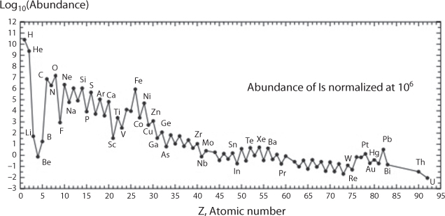
Figure 10.16 Natural relativeabundance of the elements as a function of their atomic number. (From Vanhaeckeand Kyser, 2010).
10.4.2 Isotopes and Their Relation to Greenhouse Gases
Figure 10.17 shows binding energy per nucleon for elements with atomic number greater than 20. Using this graph, scientists conclude that fission of a heavy nucleus into lighter nuclei or fusion of two H atoms into He are exo-energetic because the process results in nuclei/a nucleus characterized by a substantially higher binding energy per nucleon. Figure 10.18 shows the average binding energy for elements of mass number lower than 20. This figure shows that nuclei with an even number of protons show a higher binding energy per nucleon and thus higher stability (compare, e.g., the binding energies for 4He and 3He, 12C and 13C, and 16O and 17O.

Figure 10.17 Average bindingenergy per nucleon as a function of mass number for nuclides with a mass numberfrom 20 to 238 (From Vanhaecke and Kyser, 2010).
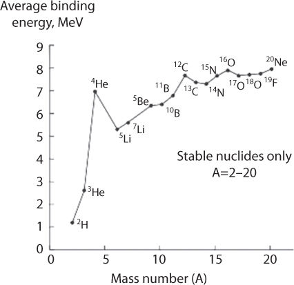
Figure 10.18 Average binding energyper nucleon as a function of mass number for nuclides with a mass number from 1 to 20. (From Vanhaecke and Kyser, 2010).
Around a mass number of 60, there is an optimum in average binding energy (Figure 10.19). Fewell (1995) indicated that the most tightly bound of the nuclei is 62Ni. This is in contradiction to previous assertion that 56Fe is the most strongly bounded nucleus. Fewell demonstrated that both 58Fe and 62Ni are more strongly bound than 56Fe. Table 10.3 shows the tabulation of the binding energy B divided by the mass number A (somewhat equivalent of atomic density). It is interesting to note that 56Fe has higher number than 52Cr, 54Cr, as well as 60Ni. It is also true that 56Fe has the highest absolute nuclear binding energy3. The optimum is explained through the fact that the more nucleons, the stronger the total strong force is in the nucleus. However, as nucleons are added, the size of the nucleus gets bigger, so the ones near the outside of the nucleus are not as tightly bound as the ones near the middle of the nucleus. Other data are shown in Tables 10.3–10.4. The binding energy per nucleon, because of the variation of the strong force with the distance, increases until the nucleus gets too big and the binding energy per nucleon starts decreasing again. This binding energy per nucleon achieves a maximum around A = 56, and the only stable isotope with that Atomic number is 56Fe. Figure 10.19 shows the nuclear binding energy per nucleon of those seven “key” elements denoted in the graph by their abbreviations (four with more than one isotope referenced). Increasing values of binding energy can be thought as the energy released when a collection of nuclei is rearranged into another collection for which the sum of nuclear binding energies is higher. As can be seen in this figure, light elements such as hydrogen release large amounts of energy (a big increase in binding energy) when combined to form heavier nuclei. This is the process of fusion. Beyond, iron, heavy elements release energy when converted to lighter nuclei—processes of alpha decay and nuclear fission. Figure 10.19 shows that the curve increases rapidly with low A, hits a broad maximum for atomic mass numbers of 50 to 60 (corresponding to nuclei in the neighbourhood of iron in the periodic table, which are the most strongly bound nuclei) and then gradually declines for nuclei with higher values of A. In this figure, iron’s ranking as optimum carries significance in terms of sustainability. In turns out iron sticks out in between toxic elements, similar to silver and gold, which also represent optimum properties. When it comes to organic applications, these optima are paramount (Bjørklund et al., 2017).
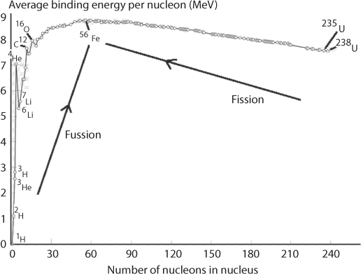
Figure 10.19 Optimum around iron.
Table 10.3 B/A Ratio for a Optimum Elements (From Wapstra and Bo, 1985).
| Nuclide | B/A (keV/A) |
| 62Ni | 8794.60 0.03 |
| 58Fe | 8792.23 0.03 |
| 56Fe | 8790.36 0.03 |
| 60Ni | 8780.79 0.03 |
Table 10.4 Most Abundant Metals and Their Concentration.
| Metal | Concentration |
Ranking |
| Aluminum | 8.1% |
1 |
| Iron | 5% |
2 |
| Calcium | 3.6% |
3 |
| Sodium | 2.8% |
4 |
| Potassium | 2.6% |
5 |
| Magnesium | 2.1% |
6 |
| Others | 0.8% |
7 |
In practical terms, it means it is the hardest to denature iron than any other element.
This variation in binding energy per nucleon also exerts a pronounced effect on the isotopic composition of the elements, especially for the light elements. “Even– even isotopes” for elements such as C and O (12C and 16O) are much more abundant than their counterparts with an uneven number of neutrons (13C and 17O). Despite the overall limited variation in binding energy per nucleon as a function of the mass number for the heavier elements, its variation among isotopes of an element may vary substantially, leading to a preferred occurrence of even–even isotopes, as illustrated by the corresponding relative isotopic abundances for elements such as Cd and Sn, as shown in Table 10.5. In both the lower (106Cd through 110Cd) and the higher (114Cd through 116Cd) mass ranges, only Cd isotopes with an even mass number occur. In addition, the natural relative isotopic abundances for 113Cd and, to a lesser extent, 111Cd are low in comparison with those of the neighboring Cd isotopes with an even mass number. Similarly, Sn, for which 7 out of its 10 isotopes are characterized by an even mass number, the isotopes with an odd mass number have a lower natural relative abundance than their neighbors. This trend continues with silicon, nitrogen, oxygen, sulphur. The only exception is hydrogen, for which uneven isotope is the stable form. Hydrogen has no neutron, deuterium has one, and tritium has two neutrons. The isotopes of hydrogen have, respectively, mass numbers of one, two, and three. Their nuclear symbols are therefore 1H, 2H, and 3H. The atoms of these isotopes have one electron to balance the charge of the one proton.
Electrons Are Fermions of Half-Integer Spin. Particles with Integer Spin Are Bosons. Fermions and Bosons Avoid Each Other
Figure 10.20 asserts the existence of number of stable isotopes of an element (upper right corner), the mass of the isotope commonly used in the delta value or alternatively the most abundant isotope (upper left corner), and the potential influence of radiogenic (RAD) and cosmogenic processes (COS) as well as mass-independent fractionation (MIF) on the stable isotope system (below the element symbol). In most cases, MIF due to nuclear volume or magnetic isotope effects has only been observed in laboratory-scale studies and has not yet been detected in natural samples (except for O, S, and Hg, marked in bold). The “traditional” stable isotope systems are marked with a red border. Elements for which high-precision stable isotope methods have been developed are marked with a bold symbol. In order to gain insight into isotopic fractionation, Hg offers an excellent case, because it has seven stable isotopes. Table 10.6 shows atomic mass and natural relative abundance of various Hg isotopes.

Figure 10.20 Periodic table with selectedelemental properties relevant for stable isotope research (from Wiederhold, 2015).
Table 10.6 Isotopic Composition of Selected Isotopes (From Vanhaecke, and Kyser, 2010 and Lide, 2002).
| Element | Atomic number, Z |
Isotope |
Natural relative abundance |
| Cd | 48 |
106Cd |
1.25 |
108Cd |
0.89 |
||
110Cd |
12.49 |
||
111Cd |
12.80 |
||
112Cd |
24.13 |
||
113Cd |
12.22 |
||
114Cd |
28.73 |
||
116Cd |
7.49 |
||
| Sn | 50 |
112Sn |
0.79 |
114Sn |
0.66 |
||
115Sn |
0.34 |
||
116Sn |
14.54 |
||
117Sn |
7.68 |
||
118Sn |
24.22 |
||
119Sn |
8.59 |
||
120Sn |
32.58 |
||
122Sn |
4.63 |
||
124Sn |
5.79 |
||
| H | 1 |
1H |
99.985 |
2H |
0.015 |
||
| C | 6 |
12C |
98.89 |
13C |
1.11 |
||
| N | 7 |
14N |
99.64 |
15N |
0.36 |
||
| O | 8 |
16O |
99.76 |
17O |
0.04 |
||
18O |
0.2 |
||
| Si | 14 |
28Si |
92.23 |
29Si |
4.67 |
||
30Si |
3.10 |
||
| S | 16 |
32S |
95.0 |
33S |
0.76 |
||
34S |
4.22 |
Figure 10.21 illustrates the influence of different fractionation mechanisms on Hg isotopes. In this figure, the arrows indicate qualitatively the influence of the mass difference effect (MDE), the nuclear volume effect (NVE), and the magnetic isotope effect (MIE) on the seven stable Hg isotopes. Mass-independent fractionation (MIF), which is defined as a measured anomaly compared with the trend of the MDE, is observed mainly for the two odd-mass isotopes 199Hg and 201Hg and can be caused either by the NVE due to their nonlinear increase in nuclear charge radii or the MIE due to their nuclear spin and magnetic moment. As can be seen from Table 10.7, natural abudance of these two isotopes are markedly lower than their corresponding ‘even-even’ counterparts, 200Hg and 202Hg, respectively. Here, MIF by the NVE and the MIE can be differentiated by the relative extent of MIF on 199Hg and 201Hg. Elements for which MIF has been detected in natural samples (only O, S, Hg) or observed in laboratory studies are marked in Figure 10.20. The relative extent of the nuclear charge radius anomalies (x/y = 1.6) causes the characteristic slope in a Δ199Hg/Δ201Hg plot for the NVE in comparison to slopes observed for Hg(II) photoreduction (1.0) and methyl-Hg photodemethylation (~1.36) due to the MIE. The magnitude of MIF due to the NVE is generally much smaller than MIF by the MIE. The MIE occurs only during kinetically controlled processes (in natural systems probably always related to photochemical reactions) whereas the NVE and the MDE occur during both kinetic and equilibrium processes. The relative importance of MDE and NVE on the overall fractionation can vary depending on the reacting species.

Figure 10.21 Schematic illustrationof fractionation mechanisms for the Hg isotope system (From Wiederhold, 2015).
Table 10.7 Mercury Isotopes.
| Isotope | Atomic mass |
Natural abundance (%) |
| 196Hg | 195.965807 |
0.15 |
| 198Hg | 197.966743 |
9.97 |
| 199Hg | 198.968254 |
16.87 |
| 200Hg | 199.968300 |
23.10 |
| 201Hg | 200.970277 |
13.18 |
| 202Hg | 201.970617 |
29.86 |
| 204Hg | 203.973467 |
6.87 |
In assessing greenhouse gas pollution, metal concentrations are paramount. Modern refining and material processing rely heavily on the use of catalysts that use metals, including heavy metals. For tracking these contaminants, isotope signatures can be used in different ways to deduce information about composition and history of environmental samples. The most important applications are source and process tracing. If the isotopic compositions of the involved end members are known and sufficiently distinct, contributions of different source materials in a sample can be quantified by mixing calculations. Figure 10.22 shows how to conduct material balance with two metal pools of opposite isotope signatures. depicts the mass balance between two metal pools of opposite isotope signatures and equal size. shows the effect of different pool sizes (pool A = 4 × pool B), whereas shows the combined effect of different pool sizes and isotope signatures. illustrates a schematic example of a natural river system for which the relative fractions of natural and anthropogenic metal sources can be quantified by metal isotope signatures. The delta (δ) value of a sample can be explained by the sum of the δ values of the mixing final products multiplied by their relative fractions of the total amount present (Equation 10.3), where where f describes the relative fraction of the involved pools A and B (fpool_A + fpool_B = 1, as per the material balance requirement).

Figure 10.22 Schematicillustration of the principles of mixing models used for source tracing with metalstable isotope signatures (From Wiederhold, 2015).
Rearranging the equation allows determining the fraction of one end product (Equation 10.4):
(10.5)

For example, if the geogenic (naturally occurring) background in a soil has an isotopic composition of +0.5‰ relative to the reference standard and the soil has been polluted by an anthropogenic source with a δ value of –1.5‰, a delta value of –1.0‰ would indicate an anthropogenic contribution of 75%. Here, of course, it is assumed that linear mixing rule is applied. As we’ll see in latter sections, real life contamination bears far greater consequence of anthropogenic materials. Chen et al. (2008) presented a case study involving Zn isotopes in the Seine River, France. This is depicted in. Chen et al. (2008) used of Zn isotope ratios as a tracer of anthropogenic contamination using an extensive collection of river water samples from the Seine River basin, collected between 2004 and 2007. The 66Zn/64Zn ratios (expressed as δ66Zn) of dissolved Zn have been measured by MC-ICP-MS after chemical separation of Zn. Significant isotopic variations (0.07–0.58 ‰) occurred along a transect from pristine areas of the Seine basin to the estuary and with time in Paris, and were found to be coherent with the Zn enrichment factor. Dissolved Zn in the Seine River displays conservative behavior, making Zn isotopes a good tracer of the different sources of contamination. Dissolved Zn in the Seine River is essentially of anthropogenic origin (>90%) compared to natural sources (<7%). Roof leaching from Paris conurbation was a major source of Zn, characterized by low δ66Zn values that are distinct from other natural and anthropogenic sources of Zn. Their study highlights the absence of distinctive δ66Zn signatures of fertilizer, compost or rain in river waters of rural areas, and therefore suggests the strong retention of Zn in the soils of the Basin. They demonstrate that Zn isotope ratios can be a powerful tool to trace pathways of anthropogenic Zn in the environment.
Estrade et al. (2010) also used source tracing for several stable isotopes of Hg. They investigated in lichens over a territory of 900 km2 in the northeast of France over a period of nine years (2001–2009). The studied area was divided into four geographical areas: a rural area, a suburban area, an urban area, and an industrial area. In addition, lichens were sampled directly at the bottom of chimneys, within the industrial area. While mercury concentrations in lichens did not correlate with the sampling area, mercury isotope compositions revealed both mass dependent and mass independent fractionation (MIF) characteristic of each geographical area. Odd isotope deficits measured in lichens were smallest in samples close to industries, with Δ199Hg of –0.15 ± 0.03 ‰, where Hg is thought to originate mainly from direct anthropogenic inputs. Samples from the rural area displayed the largest anomalies with Δ199Hg of –0.50 ± 0.03‰. Samples from the two other areas had intermediate Δ199Hg values. Mercury isotopic anomalies in lichens were interpreted to result from mixing between the atmospheric reservoir and direct anthropogenic sources. Furthermore, the combination of mass-dependent and mass independent fractionation was used to characterize the different geographical areas and discriminate the end products (industrial, urban, and local/regional atmospheric pool) involved in the mixing of mercury sources. Figure 10.23 shows how Rural Area (RA), Suburban Area (SA), Urban Area (UA), Industrial Valley (IV), Industrial sites (I). For these cases, the total Hg concentrations varied little between zones. However, the average δ202Hg value of lichens from the IV zone was significantly lighter (–2.07 ‰) than those measured for the three nonindustrial areas. Furthermore, lichens sampled at the two industrial sites (I) within IV displayed similar δ202Hg (–1.90‰) trends. This suggests that the Hg taken up by the lichens in the industrial area had different emission sources from that found in the urban, suburban, and rural areas. Furthermore, average Δ199Hg measured in IV, UA, SA, and RA were found to be significantly different from one area to another, suggesting the contribution of different mercury sources. Odd isotope deficits in lichens are believed to be representative of atmospheric Hg, which is the complementary reservoir of aquatic Hg in terms of isotope fractionation (Carignan et al., 2009). It is known that redox reactions govern mercury (Hg) concentrations in the atmosphere because fluxes (emissions and deposition), and residence times, are largely controlled by Hg speciation. Recent work on aquatic Hg photoreduction suggested that this reaction produces MIF or non-mass dependent fractionation (NMF) and that residual aquatic Hg(II)is characterized by positive δ199Hg and delta δ201Hg anomalies. Carignan et al. (2009) showed that atmospheric Hg accumulated in lichens is characterized by NMF with negative δ199Hg and δ201Hg values (–0.3 to –1 ‰), making the atmosphere and the aquatic environment complementary reservoirs regarding photoreduction and NMF of Hg isotopes. Because few other reactions than aquatic Hg photoreduction induce NMF, photochemical reduction appears to be a key pathway in the global Hg cycle. Carignan et al. (2009) also observed isotopic anomalies in several polluted soils and sediments, suggesting that an important part of Hg in these samples was affected by photoreactions and has cycled through the atmosphere before being stored in the geological environment. Thus, mercury isotopic anomalies measured in environmental samples may be used to trace and quantify the contribution of source emissions.

Figure 10.23 Average isotopicanomalies plotted as ∆199Hg vs ∆201Hg for the lichenssampled over the years 2001, 2003, 2006, 2008, and 2009 in the studied area (From Estrade et al., 2010).
They argued that this is because Hg(II) photoreduction of the aquatic reservoir yields positive ∆199Hg and ∆201Hg for residual Hg(II) with a ∆199Hg/∆201Hg close to unity, whereas Hg in lichens have negative ∆199Hg and ∆201Hg, also with a ∆199Hg/∆201Hg close to unity. The magnetic isotope effect (MIE)4 is believed to be responsible for these anomalies. Whereas lichens sampled in I, IV, RA yielded ∆199Hg/∆201Hg ratios falling on the 1:1 line (see), significant deviations were observed for all the lichens sampled in UA (average ∆199Hg/∆201Hg) 0.74 and some lichens in SA. The ratio of anomalies suggests a higher 201Hg deficit that is not in agreement with theoretical as well as experimental works which both suggest ratios between 1 and 1.3 for the MIE. This is a significant discovery because it unlocks many mysteries of quality of photosynthesis in the presence of polluted CO2.
Wiederhold (2015) pointed out that source tracing in natural systems is complicated because:
- isotopic compositions of mixing end members are not known with sufficient precision or not distinct enough;
- multiple sources contribute to a sample; and
- the isotope signature of the sample has been additionally affected by fractionating processes.
As a consequence, source tracing works best in systems with well-defined, distinct sources which are not overprinted by fractionating processes. Process tracing is based on the concept that a sample has been affected by a transformation process, causing a shift in the isotope signature. An example is the partial transformation of soluble to insoluble elemental species involving a separation of aqueous and solid phases (e.g., reduction of soluble Cr(VI) in groundwater to Cr(III) which precipitates). If the isotopic enrichment factor (ε) for the transformation process is known, the extent of reaction can be quantified from the heavy isotope enrichment in the remaining reactant using a Rayleigh model. The Rayleigh model assumes an exponential relationship that describes the partitioning of isotopes between two reservoirs as one reservoir decreases in size. This is reasonable if the material is continuously removed from a mixed system containing molecules of two or more isotopic species, the fractionation accompanying the removal process at any instance is described by a constant fractionation factor. However, in a natural setting, such conditions rarely prevail.
In understanding atmospheric pollution, the notion of Redox processes is helpful.
These processes, involving stable isotope fractionation between different oxidation states of metals represent one of the most important sources of isotopic variability in natural samples. Because nature is continuous, such oxidation is ubiquitous. However, an in-depth study is rare. Interestingly, the equilibrium isotope effect between aqueous Fe(II) and Fe(III) is one of the best studied systems (Wiederhold, 2015). Theoretical studies provide a fundamental basis for equilibrium isotope fractionation between oxidation states of metals, such as Cr,97 Cu,98,55 Zn,99 Se,100 Hg,41 generally predicting an enrichment of heavy isotopes in the oxidized species, except for U,42 where an inverse redox effect is observed due to the dominance of the NVE. Note, here, that the use of NVE to explain such behaviour is not satisfactory. Such description is not necessary with our galaxy model discussed in previous chapters.
Of relevance is the fact that anthropogenic processing can induce redox changes for metals. For example, ore smelting and roasting, the production of elemental metals or engineered nanoparticles for industrial purposes, and combustion processes can cause isotope fractionation due to redox effects (e.g., Zn,101–104 Cd,105,106 Hg107,108,78), which may be preserved if the process is incomplete and isotopically fractionated metal pools with different oxidation states are released into the environment. Practically all industrial processes have such oxidation in place. Also, the most popular catalysts as well as pesticides contain these metallic products. Furthermore, electroplating can cause large isotope effects due to redox processes. More importantly, electroplated materials may constitute isotopically distinct metal sources released to the environment as metal wastes and mobilized via corrosion processes.
Significant pollution through metal isotope fractionation can take place with the formation of aqueous solution complexes and the binding of metals to functional groups of organic matter. This can take place under thermodynamic imbalances. Even without redox changes, the coordination of ligand complexes can be distinct enough to cause significant metal isotope fractionation. This is an extremely important phenomenon during photosynthesis. Numerous experimental observations indicate that heavy isotope enrichments are observed in organically complexed species compared with free aqueous species in the presence of stronger bonding environments (e.g., Fe,112,116 Zn,113 Cu114,115). In contrast, organic thiol complexes have been shown to be enriched in light Hg isotopes, consistent with theoretical calculations predicting light Hg isotope enrichments in coordination with reduced sulfur, compared with hydroxyl or chloride ligands in solution (Wiederhold, 2015). Similarly, organic complexes enriched in light Mg isotopes were explained by a longer bond length compared with corresponding inorganic complexes. None of these studies, however, identifies long-term impact on the organic matter and how the resulting oxidation products are contaminated.
The environmental fate of metals is often strongly controlled by sorption. In most cases, the magnitude of fractionation is smaller than for redox effects of the same element. For most metals, isotopic enrichment factors of <1 o/oo were determined for sorption, but larger values were found in some cases (e.g., Mo132). Fractionation during sorption is mostly governed by differences in bonding environment between dissolved and sorbed phases or solution species sorbing to a different extent. It is often difficult to verify that equilibrium conditions have been established, and desorption rates are often much slower than adsorption rates, delaying the attainment of isotopic equilibrium. Many studies were conducted with metal oxides (mainly Fe and Mn (oxyhydr)oxides), but other sorbents (e.g., clay minerals, bacteria) were also used. A first summary of metal isotopic enrichment factors during sorption to metal oxides 134 suggested that sorption of cationic species (e.g., Fe, Cu, Zn) causes heavy isotope enrichments in the sorbed phases and sorption of anionic metal species (e.g., Ge,135 Se,136 Mo,132 U137) results in light isotope enrichments in the sorbed phases. However, newer studies also reported light isotope enrichments in the sorbed phase for cationic metal species (e.g., Ca,138 Cu,139 Cd,140 Hg51). Data are limited on the topic of kinetic isotope effects during adsorption and desorption of metals. For instance, Miskra et al. (2014), using enriched Hg isotope tracers, revealed slow kinetics and incomplete exchange of Hg(II) with organic complexes and mineral surfaces, suggesting that kinetic isotope effects during the initial sorption step may be partially preserved in the presence of non-exchangeable pools. They discovered that mobility and bioavailability of toxic Hg(II) in the environment strongly depends on its interactions with natural organic matter (NOM) and mineral surfaces. They investigated the exchange of Hg(II) between dissolved species (inorganically complexed or cysteine-, EDTA-, or NOM-bound) and solid-bound Hg(II) (carboxyl-/thiol-resin or goethite) over 30 days under constant conditions (pH, Hg and ligand concentrations). The Hg(II)-exchange was initially fast, followed by a slower phase, and depended on the properties of the dissolved ligands and sorbents. The time scales required to reach equilibrium with the carboxyl-resin varied greatly from 1.2 days for Hg(OH)2 to 16 days for Hg(II)–cysteine complexes and approximately 250 days for EDTA-bound Hg(II). Other experiments could not be described by an equilibrium model, suggesting that a significant fraction of total-bound Hg was present in a non-exchangeable form (thiol-resin and NOM: 53–58%; goethite: 22–29%). Based on the slow and incomplete exchange of Hg(II) described in that study, Miskra et al. (2014) suggested that kinetic effects must be considered to a greater extent in the assessment of the fate of Hg in the environment and the design of experimental studies, for example, for stability constant determination or metal isotope fractionation during sorption.
The arctic represents an interesting test ground for observing atmospheric pollution with heavy metals. Studies show that atmospheric Hg deposition has increased about 3-fold from pre-industrialized background levels (Fitzgerald et al., 2014). Representing about 26% of the global land surface area, polar regions are unique environments with specific physical, chemical, and biological processes affecting pollutant cycles including that of Hg (Douglas et al., 2012). Trace gas exchanges between the atmosphere and the tundra are modulated by sinks and sources below and within snowpack, by snow diffusivity, snow height, and snow porosity (Agnan et al., 2018). Agnan et al. (2018) investigated Hg dynamics in an interior Arctic tundra snowpack in northern Alaska during two winter seasons. Using a snow tower system to monitor Hg trace gas exchange, they observed consistent concentration declines of gaseous elemental Hg (Hg0 gas) from the atmosphere to the snowpack to soils. They found no evidence of photochemical reduction of HgII to Hg0 gas in the tundra snowpack, with the exception of short periods during late winter in the uppermost snow layer. Chemical tracers showed that Hg was mainly associated with local mineral dust and regional marine sea spray inputs. Mass balance calculations showed that the snowpack represents a small reservoir of Hg, resulting in low inputs during snowmelt. Taken together, the results from this study suggest that interior Arctic snowpacks are negligible sources of Hg to the Arctic.
Precipitations can help with isotope enrichments. Isotope fractionation during precipitation can be described by a Rayleigh model, the shortcomings of which are discussed earlier. For precipitates, it means the process unidirectional and no significant re-equilibration of the formed precipitate with the solution phase occurs. It is generally understood that kinetic and equilibrium isotope fractionation is a complex process that has can play a pivotal role in view of the fact that aqueous phase is connected to organic matters. The formation of aqueous solution complexes and the binding of metals to functional groups of organic matter sets up possibilities for metal isotope fractionation. Even without redox changes, the coordination of ligand complexes can be distinct enough to cause significant metal isotope fractionation. In general, it has been observed that heavy isotope enrichments take place within organically complexed species compared with free aqueous species and explained by their stronger bonding environments (e.g., Fe,112,116 Zn,113 Cu114,115).
Metals are involved in biological cycling. However, biological processes behave different in presence of artificial chemicals from how they behave in presence of natural chemicals. In either cases, significant metal isotope fractionation will occur through redox change, complexation, sorption, diffusion, etc. Many biological processes are kinetically controlled (e.g., bond-breaking in enzymatic reactions) and may thus induce kinetic isotope effects. Although New Science rarely acknowledges the fact that these effects are preserved in signatures of natural samples, the use of the galaxy model, it becomes evident, each of these effects will carry a signature that is detectable by the natural system.
What is missing in today’s literature is answer to the question what role does artificial chemicals play in creating atmospheric pollution. What we know is natural materials are available in certain proportion and each material has a function for overall welfare of humans. From the above discussion, we know that it is easier to denature elements that are heavier than iron and by denaturing them they become agents of pollution and start to act as a ‘cancer’ to the environment. In producing denatured metals, we create these ‘agents’ that pollute much bigger fraction of the atmosphere. Figure 10.24 shows the amount of emissions caused by the production of various metals. This figure shows the global production and consumption of selected toxic metals during 1850–1990.
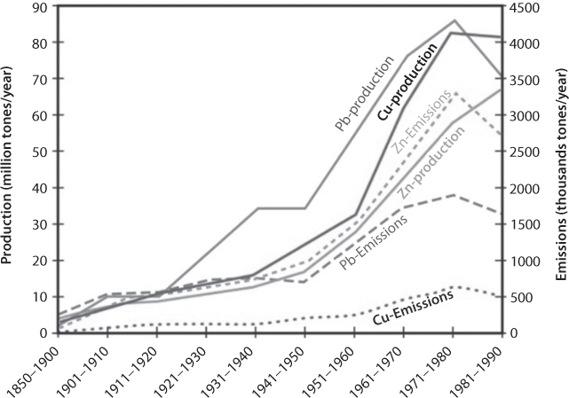
Figure 10.24 The global productionand consumption of selected toxic metals during 1850–1990 (From Jaishankar et al., 2014).
The most commonly found heavy metals in waste water include arsenic, cadmium, chromium, copper, lead, nickel, and zinc, all of which cause risks for human health and the environment. Heavy metals enter the surroundings by natural means and through human activities. Various sources of heavy metals include soil erosion, natural weathering of the earth’s crust, mining, industrial effluents, urban runoff, sewage discharge, insect or disease control agents applied to crops, and many others (Morais et al., 2012).
Each of these metals have crucial biological functions in plants and animals, yet the artificial (e.g., processed with artificial energy source or chemicals) version of them become inherently toxic to the organism. Previous research has found that oxidative deterioration of biological macromolecules is primarily due to binding of heavy metals to the DNA and nuclear proteins (Flora et al., 2008).
Consequence of such effects on organic matter must be reflected on the overall greenhouse gas emission. Take for instance, the case of N2O emissions. Majority of that emission is derived from nitrogen fertilization and indirect emissions. These are entirely toxic to the environment. Most of it would be rejected by the ecosystem and some of them get assimilated in organic matter, it will only create amplified pollution by passing through increased amount of biomass in an organic body (Galloway et al. 2008). Generally, for every 1000 kg of applied nitrogen fertilizers, it is estimated that around 10–50 kg of nitrogen will be lost as N2O from soil, and the amounts of N2O emissions increase exponentially relative to the increasing nitrogen inputs (Shcherbak et al., 2014). Given that farmlands and fertilizer application are predicted to increase by 35–60% before 2030, global N2O concentrations are likely to continuously rise in the coming decades and it is expected that agricultural soils will contribute up to 59% of total N2O emissions in 2030 (Hu et al., 2015). This is shown in Figure 10.25.
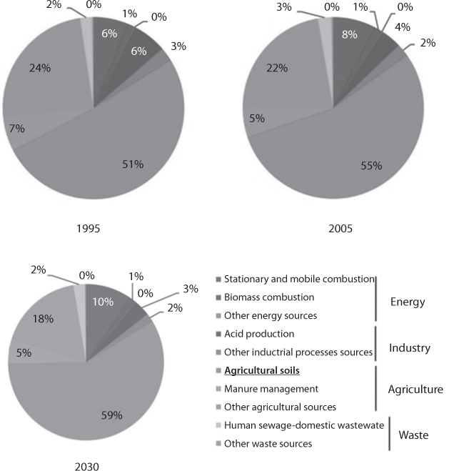
Figure 10.25 Global N2Oemissions from various sources in 1995, 2005 and 2030. ‘Other energy sources’here includes waste combustion, fugitives from solid fuels, natural gas and oilsystems. ‘Other industrial processes sources’ includes metal production, solvent and other product use. ‘Other agricultural sources’ includes fieldburning of agricultural residues and prescribed burning of savannas. ‘Otherwaste sources’ includes miscellaneous waste handling processes. (From Hu etal., 2015)
Figure 10.26. shows how intricately all materials, natural and artificial, form a close cycle. It shows everytime there is anartificial molecule in the system, its effects continue to multiply.
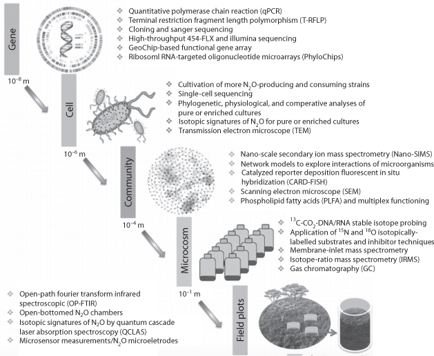
Figure 10.26 A proposedmethodological framework proposed by Hu et al. (2015).
10.5 A New Approach to Material Characterization
Khan and Islam (2012) introduced a new approach to material characterization in order to highlight the damages caused by unsustainable practices. It was applied to agricultural products. As a first stab in the new direction that the approach discussed in that work opens up, consider the following cases, involving the cultivation of a crop:
Case A) Crop grown without any fertilizer. Land is cultivated with naturally available organic fertilizers (from flood, etc.) Consider the crop yield to be Y0. This is the baseline crop yield.
Case B) Crop grown with organic fertilizer (e.g., cow dung in Asia, guano in Americas). Consider the crop yield to be Y1.
Case C) Crop grown with organic fertilizer and natural pesticide (e.g., plant extract, limestone powder, certain soil). Consider the crop yield to be Y2.
Case D) Crop grown with chemical fertilizer (the ones introduced during “green revolution”). Consider the crop yield to be Y3.
Case E) Crop grown with chemical fertilizer and chemical pesticide. Consider the crop yield to be Y4.
Case F) Crop grown with chemical fertilizer, chemical pesticide, and genetically modified seeds. Consider the crop yield to be Y5.
Case G) Crop grown with chemical fertilizer, genetically modified seeds and genetically modified pesticide. Consider the crop yield to be Y5.
It is well known that for a given time, Y5 > Y4>Y3>Y2>Y1>Y0. If profit margin is used as a criterion, practices that give the most crop yield would be preferred. Of course a t a time (t= “right now”‘), this is equivalent to promoting “‘crops are crops”‘. Aside from any considerations of product quality, which might suffer great setback at a time other than ‘t= “right now”‘, their higher yield directly relates to higher profit. Historically, a portion of the marketing budget is allocated to obscure the real quality of a product in order to linearize the relationship between yields and profit margins. The role of advertisement in this is to alter peoples’ perception, which is really a euphemism for forcing people to exclusively focus on the short-term. In this technology development, if natural rankings are used, Cases D through G would be considered to be progressively worse in terms of sustainability. If this is the ranking, how then can one proceed with that characterization of a crop that must have some sort of quantification attached to it? For this, an sustainability index is introduced in the form of a Dirac δ function, δ (s), such that:
δ(s) = 1, if the technology is sustainable; and
δ(s) = –1, if the technology is not sustainable.
Here, sustainability criterion of Khan and Islam (2007) was used. A process is aphenomenal if it doesn’t meet the sustainability criterion and it assumes a δ value of –1. Therefore, the adjustment we propose in revising the crop yield is as follows:
(10.6)
Here Y stands for the actual crop yield, something recorded at present time. Note that Yreal has a meaning only if future considerations are made. This inclusion of the reality index forces decision makers to include long-term considerations. The contribution of a new technique is evaluated through the parameter that quantifies quality as, Qreal (stands for real quantity), given as:
(10.7)
For unsustainable techniques, the actual quantity, Y will always be stheory is dependent on a series of assumptions whichmaller than Y0. The higher the apparent crop yield for this case, the more diminished the actual quality. In addition to this, there might be added quality degradation that is a function of time. Because an unsustainable technology continues to play havoc on nature for many years to come, it is reasonable to levy this cost when calculations are made. This is done through the function, L (t). If the technique is not sustainable, the quality of product will continue to decline as a function of time. Because quality should be reflected in pricing, this technique provides a basis for a positive correlation between price and quality. This is a sought-after goal that has not yet been realized in the post-industrial revolution era (Zatzman and Islam, 2007b). At present, price vs. quality has a negative slope, at least during the early phase of a new technology. Also, the profit margin is always inversely proportional to the product quality. Nuclear energy may be the cheapest, but the profit margin of the nuclear energy is the highest. Herbal medicines might be the only ones that truly emulate nature which has all the solutions, but the profit margins are the lowest in herbal medicines. Today, organic honey (say from the natural forest) is over 10 times more expensive than farm honey when it is sold in the stores. However, people living close to natural habitats do have access to natural honey free of cost, but the profit margin in farm honey is still the highest. In fact, pasteurized honey from Australia is still one expensive locally available unadulterated honeys (from a local source, but not fully organic) in the Middle East.
The aim of this approach is to establish in stepwise manner a new criterion that can be used to rank product quality, depending on how real (natural) the source and the pathways are. This will distinguish between organic flower honey and chemical flower honey, use of antibiotics on bees, electromagnetic zones, farming practices, sugar for bees, as well as numerous intangibles. This model can be used to characterize any food product that makes the value real.
In this context, the notion of mass balance needs to be rethought, so that infinite dimensions (using t as a continuous function) can be handled. What we have to establish is the dynamism of the mass-energy-momentum balance at all scales, and the necessity for non-linear methods of computing just where the balance is headed at any arbitrarily-chosen point. Non-linear needs to be taken and understood to mean that there is no absolute boundary. There is only the relative limit between one state of computation and other computational states. Differences between states of computation are not necessarily isomorphic (in 1:1 correspondence) with actual differences between states of nature. Knowledge gathered about the former is only valuable as one of a number of tools for determining more comprehensively what is actually going on with the latter.
What does it mean to capture intangibles and make sense of them without throwing away tangibles? The climate change conundrum suggests that problems of this type require considering all energy sources and all masses, still using the mass balance equation, for example, but in this redefined form. Consider in particular, what is involved in the producing CO2. Every living organism emits certain amount of CO2 after utilizing naturally available oxygen from the atmosphere. During that process, every molecule of CO2 will never be by itself and invariably be accompanied with every type of molecules, including artificial ones that will act as a ‘cancer’ to the organism. When the produces CO2 encounters vegetation, photosynthesis will be attempted and immediately the photosynthesis will be affected by every molecule that accompanied the CO2 molecule in question. How can we then expect a natural system (such as plant) to not consider all the accompanying molecules and ‘look’ at the CO2 as independent of the other molecules? It is indeed an absurd concept.
Modeling nature as it is, nevertheless, would still involve collecting and collating a large amount of data that takes at least initially the form of apparently discrete events. The temptation is to go with statistical methods, as has been the case for the ‘97% consensus’ group. This, however, is also one of those points of bifurcation where the actual content of the data of nature has to be taken into account. The fact that events recorded from some processes in nature may be observed as discrete and distinct, does not mean or necessarily prove that these events are stochastically independent.
According to the prevailing theories of mathematical probability, it is legitimate to treat a sufficiently very large number of similar events, e.g., tossing dice, as though these discrete events approximated some continuous process. There is a “Strong Law of Large Numbers” [SLLN] and a more relaxed, less bounded version known as the “Weak Law of Large Numbers” [WLLN], which propose a mathematical justification for just such a procedure (Kolmogorov, 1930).
When we are examining moments in nature, however, which are defined to some extent by some actual passage of time, apart from continuous fluid flow or other motion that is similarly continuous in time, how legitimate or justifiable can it be to approximate discrete events using “nice”, i.e., tractable, exponential functions that are continuous and defined everywhere between negative and positive infinity? If the event of interest, although in itself discrete, cycles in a continuum, it would seem that there should arise no particular problem (Of course, there is also no problem for any phenomenon that has been human-engineered and whose data output is to that extent based on human artifice rather than nature).
However, the fact that some recorded data of any large number of such discrete events, exists cannot be taken as sufficient. It is also necessary to be able to establish that the observations in question were recorded in the same time continuum, not in different continua attended by a different set or sets of external surrounding [boundary] conditions. To group and manipulate such data with the tools of mathematical statistics, however, as though the conditions in which the phenomena actually occurred were a matter of indifference, and cannot be justified on the basis of invoking the logic of either the SLLN or WLLN. The continuity of the number and of the characteristics of the abstract construct known as “the real numbers”, which form the basis of the SLLN and WLLN, has nothing inherently to do with whether natural phenomena being studied or measured are themselves, actually continuous or occurring within a continuum possessing cyclical features. Some definite yet indeterminate number of such data measurements of the same event — recorded, however, in unrelated and distinct times and places — would likely be so truly “discrete” as not to form part of any actual time-continuum in nature.
Mathematically, working purely with numbers, it may not matter whether there was any physical continuum within which discrete data points were being recorded. In such cases, the strictures of the SLLN and WLLN are adequate, and the approximation of the discrete by the continuous generates no problem. But what we can “get away with” dealing in pure numbers is one thing. Interpreting the results in terms of physical realities is another matter. When it comes to interpreting the results in terms of physical realities in the natural environment in which the phenomena of interest were observed and recorded, the absence of a physical continuum means that any conclusions as to the physics or nature-science that may underlie or may also be taking place will, and indeed must necessarily, be aphenomenal. Correlations discovered in such data may very well be aphenomenal. Any inferences as to possible “cause-effect” relationships will also be aphenomenal.
Assuming abstract numerical continuity on the real-number line for an extremely large number of discrete data points generated for the same abstract event, lets us overlay another level of information atop the actual discrete data because the tendency of the numerical data purely as numbers is isomorphic to the envelope generated by joining the discrete data points. This isomorphism, however, is precisely what cannot be assumed in advance regarding the underlying phenomenon, or phenomena, generating whatever observations are being recorded from some actual process taking place in nature.
What does this mean? When it comes to the science of nature, the mere fact of some event’s occurrence is necessary information, but in itself this information is also insufficient without other additional “meta”-data about the pathway(s) of the event’s occurrence, etc. There are strong grounds here for treating with the greatest skepticism a wide range of quantitative projections generated by all the current models of global warming and climate changes.
10.5.1 Removable Discontinuities: Phases and Renewability of Materials
By introducing time spans of examination unrelated to anything characteristic of the phenomenon itself being observed in nature, discontinuities appear. These are entirely removable, but they appear to the observer as finite limits of the phenomenon itself, and as a result, the possibility that these discontinuities are removable is not even considered. This is particularly problematic when it comes to the matter of phase transitions of matter and the renewability or non-renewability of energy.
The transition between the states of solid, liquid and gas in reality is continuous, but the analytical tools formulated in classical physics are anything but; each P-V-T model applies to only one phase and one composition, and there is no single P-V-T model applicable to all phases (Cismondi and Mollerup, 2005). Is this an accident? Microscopic and intangible features of phase-transitions have not been taken into account. As a result, this limits the field of analysis to macroscopic, entirely tangible features and modeling therefore becomes limited to one phase and one composition at a time.
When it comes to energy, everyone has learned that it comes in two forms—renewable and nonrenewable. If a natural process is being employed, however, everything must be “renewable” by definition in the sense that, according to the Law of Conservation of Energy, energy can be neither created nor destroyed. Only the selection of the time frame misleads the observer into confounding what is accessible in that finite span with the idea that energy is therefore running out. The dead plant material that becomes petroleum and gas trapped underground in a reservoir is being added to continually, but the rate at which it is being extracted has become set according to an intention that has nothing to do with what the optimal timeframe in which the organic source material could be renewed. Thus, “non-renewability” is not any kind of absolute fact of nature. On the contrary, it amounts to a declaration that the pathway on which the natural source has been harnessed is anti-Nature.
10.5.2 Rebalancing Mass and Energy
Mass and energy balances inspected in depth disclose intention as the most important parameter, as the sole feature that renders the individual accountable to, and within, nature. This is rife with serious consequences for the black-box approach of conventional engineering, because a key assumption of the black-box approach stands in stark and howling contradiction to one of the key corollaries of that most fundamental principle of all: the Law of Conservation of Matter.
In fact, this is only possible if there is no leak anywhere and no mass can flow into the system from any other point. However,
mass can flow into the system from any other point – thereby rendering the entire analysis a function of tangible measurable quantities; i.e., a “science” of tangibles-only Figure 10.27.
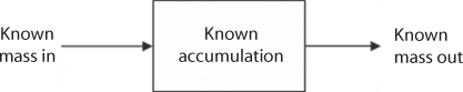
Figure 10.27 Conventional Mass Balanceequation incorporating only tangibles.
The mass conservation theory indicates that the total mass is constant. It can be expressed as follows:
(10.8)
where m = mass and i is the number from 0 to ∞.
In the true sense, this mass balance encompasses mass from macroscopic to microscopic and detectable to undetectable; i.e., from tangible to intangible. Therefore, the true statement should be as illustrated in Figure 10.28:
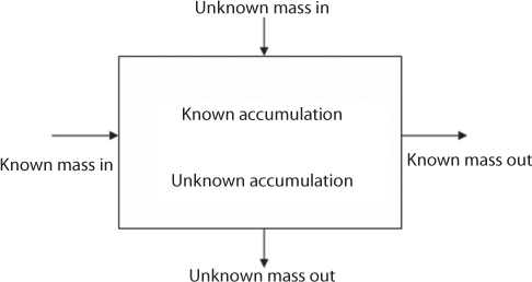
Figure 10.28 Mass-balance equationincorporating tangibles and intangibles.
(10.9)

The unknown masses and accumulations are neglected, which means they are considered to be equal to zero.
Every object has two masses:
- Tangible mass.
- Intangible mass, usually neglected.
Then, equation [3.5] becomes:
(10.10)

The unknowns can be considered intangible, yet essential to include in the analysis as they incorporate long-term and other elements of the current timeframe.
In nature, the deepening and broadening of order is continually observed, with many pathways, circuits and parts of networks being partly or even completely repeated and the overall balance being further enhanced. Does this actually happen as arbitrarily as conventionally assumed? A little thought suggests this must take place principly as a result and/or as a response to human activities and the response of the environment to these activities and their consequences. Nature itself has long established its immediate and unbreachable dominion over every activity and process of everything in its environment, and there is no other species that can drive nature into such modes of response. In the absence of the human presence, nature would not be provoked into having to increase its order and balance, and everything would function in the “zero net waste” mode.
An important corollary of the Law of Conservation of Mass, that mass can be neither created nor destroyed, is that there is no mass that can be considered in isolation from the rest of the universe. Yet, the black-box model clearly requires just such an impossibility. Since, however, human ingenuity can select the time frame in which such a falsified “reality” will be exactly what the observer perceives, the model of the black box can be substituted for reality and the messy business of having to take intangibles into account is foreclosed once and for all.
10.5.3 Energy: Toward Scientific Modeling
There have been a number of theories developed in the past centuries to define energy and its characteristics. However, none of the theories is enough to describe energy properly. All of the theories are based on much idealized assumptions which have never existed practically. Consequently, the existing model of energy and its relation to others cannot be accepted confidently. For instance, the second law of thermodynamics depends on Carnot cycle in the classical thermodynamics where none of the assumptions of Carnot’s cycle exists in reality. Definitions of ideal gases, reversible processes and adiabatic processes used in describing the Carnot’s cycle are imaginary. In 1905, Einstein came up with his famous equation, E=mc2 which states an equivalence between energy (E) and relativistic mass (m), in direct proportion to the square of the speed of light in a vacuum (c2). However, the assumptions of constant mass and the concept of vacuum do not exist in reality. Moreover, this theory was developed on the basis of Planck’s constant which was derived from black body radiation. Perfectly black bodies don’t even exist in reality. So it is found that the development of every theory is dependent on a series of assumptions which do not exist in reality.
The scientific approach must include restating the mass balance.
For whatever else remains unaccounted for, the mass balance equation, which in its conventional form necessarily falls short of explaining the functionality of nature coherently as a closed system, is supplemented by the energy balance equation.
For any time, the energy balance equation can be written as:
(10.11)

Where a is the activity equivalent to potential energy.
In the above equation, only potential energy is taken into account. Total potential energy, however, must include all forms of activity, and here once again, a large number of intangible forms of activity, e.g., the activity of molecular and smaller forms of matter, cannot be “seen” and accounted for in this energy balance. The presence of human activity introduces the possibility of other potentials that continually upset the energy balance in nature. There is overall balance but some energy forms, e.g., electricity (either from combustion or nuclear sources), would not exist as a source of useful work except for human intervention which continually threaten to push this into a state of imbalance.
In the definition of activity, both time and space are included. The long term is defined by time being taken to infinity. The “zero waste” condition is represented by space going to infinity. There is an intention behind each action and each action is playing an important role in creating overall mass and energy balance.
The role of intention is not to create a basis for prosecution or enforcement of certain regulations. It is rather to provide the individual with a guideline. If the product or the process is not making things better with time, it is fighting nature – a fight that cannot be won and is not sustainable. Intention is a quick test that will eliminate the rigorous process of testing feasibility, long-term impact, etc. Only with “good” intention can things improve with time. After that, other calculations can be made to see how fast the improvements will take place.
In clarifying the intangibility of an action or a process, the equation has some constant which is actually an infinite series:
(10.12)
If each term of Equation (3.8) converges, it will have a positive sign, indicating intangibility; hence the effect of each term thus becomes important for measuring the intangibility overall. On this path, it should also become possible to analyze the effect of any one action and its implications for sustainability overall as well.
It can be inferred that man-made activities are not enough to change the overall course of nature. Failure up until now, however, to include an accounting for the intangible sources of mass and energy, has brought about a state of affairs in which, depending on the intention attached to such interventions, the mass-energy balance can either be restored and maintained over the long-term, or increasingly threatened and compromised in the short- term. In the authors’ view, it would be far better to develop the habit of investigating Nature and the prospects and possibilities it offers Humanity’s present and future, by considering time t at all scales, going to infinity, and giving up once and for all the habit of resorting to time scales that appear to serve some immediate ulterior interest in the short-term but which in fact have nothing to do with natural phenomena, must therefore lead to something that will be anti-Nature in the long-term and the short-term.,
The main obstacle to discussing and positioning the matter of human intentions within the overall approach to the Laws of Conservation of Mass, Energy and Momentum stems from notions of the so-called “heat death” of the universe, predicted in the 19th century by Lord Kelvin and enshrined in his Second Law of Thermodynamics. In fact, however, this idea that the natural order must “run down” due to entropy, eliminating all sources of “useful work,” naively attempts to assign what amounts to a permanent and decisive role for negative intentions in particular without formally fixing or defining any role whatsoever for human intentions in general. Whether they arise out of the black-box approach of the mass-balance equation or the unaccounted missing potential energy sources in the energy balance equation, failures in the short-term become especially highly consequential when they are used by those defending the status quo to justify anti-Nature “responses” of the kind well-described elsewhere as typical examples of “the roller coaster of the Information Age” (Islam et al., 2003).
10.5.4 The Law of Conservation of Mass and Energy
Lavoisier’s first premise was “mass cannot be created or destroyed”. This assumption does not violate any of the features of Nature. However, his famous experiment had some assumptions embedded in it. When he conducted his experiments, he assumed that the container was sealed perfectly — something that would violate the fundamental tenet of Nature that an isolated chamber can be created. Rather than recognizing the aphenomenality of the assumption that a perfect seal can be created, he “verified” his first premise (law of conservation of mass) “within experimental error”.
Einstein’s famous theory is more directly involved with mass conservation. He derived E = mc2 using the first premise of Planck (1901). However, in addition to the aphenomenal premises of Planck, this famous equation has its own premises that are aphenomenal. However, this equation remains popular and is considered to be useful (in the pragmatic sense) for a range of applications, including nuclear energy. For instance, it is quickly deduced from this equation that 100 kJ is equal to approximately 10-9 gram. Because no attention is given to the source of the matter nor of the pathway, the information regarding these two important intangibles is wiped out from the conventional scientific analysis. The fact that a great amount of energy is released from a nuclear bomb is then taken as evidence that the theory is correct. By accepting this at face value (heat as a one-dimensional criterion), heat from nuclear energy, electrical energy, electromagnetic irradiation, fossil fuel burning, wood burning or solar energy, becomes identical.
In terms of the well-known laws of conservation of mass (m), energy (E) and momentum (p), the overall balance, B, within Nature may be defined as some function of all of them:
(10.13)
The perfection without stasis that is Nature means that everything that remains in balance within it is constantly improving with time. That is:
(10.14)
If the proposed process has all concerned elements so that each element is following this pathway, none of the remaining elements of the mass balance discussed later will present any difficulties. Because the final product is being considered as time extends to infinity, the positive (“<0”) direction is assured.
10.5.5 Avalanche Theory
A problem posed by Newton’s Laws of Motion, however, is the challenge they represent of relying upon and using the principle of energy-mass-momentum conservation. This principle is the sole necessity and the sufficient condition for analyzing and modeling natural phenomena in situ, so to speak — as opposed to analyzing and generalizing from fragments captured or reproduced under controlled laboratory conditions.
The underlying problem is embedded in Newton’s very notion of motion as the absence of rest, coupled with his conception of time as the duration of motion between periods of rest. The historical background and other contradictions of the Newtonian system arising from this viewpoint are examined at greater length in Abou-Kassem et al. (2008), an article that was generated as part of an extended discussion of, and research into, the requisites of a mathematics that can handle natural phenomena unadorned by linearizing or simplifying assumptions. Here the aim is to bring forward those aspects that are particularly consequential for approaching the problems of modeling phenomena of Nature, where “rest” is impossible and inconceivable.
Broadly speaking, it is widely accepted that Newton’s system, based on his three laws of motion accounting for the proximate physical reality in which humans live on this Earth coupled with the elaboration of the principle of universal gravitation to account for motion in the heavens of space beyond this Earth, makes no special axiomatic assumptions about physical reality outside the scale on which any human being can observe and verify for himself / herself (i.e., the terrestrial scale on which we go about living daily life). For example, Newton posits velocity, v, as a change in the rate at which some mass displaces its position in space; s, relative to the time duration; t, of the motion of the said mass. That is:
(10.15)
This is no longer a formula for the average velocity, measured by dividing the net displacement in the same direction as the motion impelling the mass by the total amount of time that the mass was in motion on that path. This formula posits something quite new (for its time, viz., Europe in the 1670s), actually enabling us to determine the instantaneous velocity at any point along the mass’s path while it is still in motion.
The “v” that can be determined by the formula given in equation [4.3] above is highly peculiar. It presupposes two things. First, it presupposes that the displacement of an object can be derived relative to the duration of its motion in space. Newton appears to cover that base already by defining this situation as one of what he calls “uniform motion”. Secondly, however, what exactly is the time duration of the sort of motion Newton is setting out to explain and account for? It is the period in which the object’s state of rest is disturbed, or some portion thereof. This means the uniformity of the motion is not the central or key feature. Rather, the key is the assumption in the first place that motion is the opposite of rest.
In his First Law, Newton posits motion as the disturbance of a state of rest. The definition of velocity as a rate of change in spatial displacement relative to some time duration means that the end of any given motion is either the resumption of a new state of rest or the starting-point of another motion that continues the disturbance of the initial state of rest. Furthermore, only to an observer external to the mass under observation can motion appear as the disturbance of a state of rest and can a state of rest appear as the absence or termination of motion. Within nature, meanwhile, is anything ever at rest? The struggle to answer this question exposes the conundrum implicit in the Newtonian system: everything “works” — all systems of forces are “conservative” — if and only if the observer stands outside the reference frame in which a phenomenon is observed.
In Newton’s mechanics, motion is associated not with matter-as-such, but only with force externally applied. Inertia, on the other hand, is definitely ascribed to mass. Friction is considered only as a force equal and opposite to that which has impelled some mass into motion. Friction, in fact, exists at the molecular level, however, as well as at all other scales — and it is not a force externally applied. It is a property of matter itself. It follows that motion must be associated fundamentally not with force(s) applied to matter, but rather with matter itself. Although Newton nowhere denies this possibility, his First Law clearly suggests that going into motion and ceasing to be in motion are equal functions of some application of force external to the matter in motion; i.e., motion is important relative to some rest or equilibrium condition.
Following Newton’s presentation of physical reality in his Laws of Motion, if time is considered mainly as the duration of motion arising from force(s) externally applied to matter, then it must cease when an object is “at rest”. Newton’s claim in his First Law of Motion that an object in motion remains in (uniform) motion until acted on by some external force appears at first to suggest that, theoretically, time is taken as being physically continual. It is mathematically continuous, but only as the independent variable, and indeed, according to equation (4.3) above, velocity v becomes undefined if time-duration t becomes 0. On the other hand, if motion itself ceases— in the sense of ∂s, the rate of spatial displacement, going to 0 — then velocity must be 0. What has then happened, however, to time? Where in nature can time be said either to stop or to come to an end? If Newton’s mechanism is accepted as the central story, then many natural phenomena have been operating as special exceptions to Newtonian principles. While this seems highly unlikely, its very unlikelihood does not point to any way out of the conundrum.
This is where momentum p, and — more importantly — its “conservation”, comes into play. In classically Newtonian terms:
(10.16)
Hence
(10.17)
If the time it takes for a mass to move through a certain distance is shortening significantly as it moves, then the mass must be accelerating. An extreme shortening of this time corresponds therefore to a proportionately large increase in acceleration. However, if the principle of conservation of momentum is not to be violated, either:
- the rate of its increase for this rapidly accelerating mass is comparable to the increase in acceleration — in which case the mass itself will appear relatively constant and unaffected; or
- mass itself will be increasing, which suggests that the increase in momentum will be greater than even that of the mass’s acceleration; or
- mass must diminish with the passage of time, which implies that any tendency for the momentum to increase also decays with the passage of time.
The rate of change of momentum (∂p/∂t) is proportional to acceleration (the rate of change in velocity, as expressed in the ∂2s/∂t2 term) experienced by the matter in motion. It is proportional as well to the rate of change in mass with respect to time (the ∂m/∂t term). If the rate of change in momentum approaches the acceleration undergone by the mass in question, i.e., if ∂p/∂t → ∂2 s/∂t2, then the change in mass is small enough to be neglected. On the other hand, a substantial rate of increase in the momentum of some moving mass — on any scale much larger than its acceleration — involves a correspondingly substantial increase in mass.
The analytical standpoint expressed in equation (4.4) and equation (4.5) above work satisfactorily for matter in general, as well as for Newton’s highly specific and indeed peculiar notion of matter in the form of discrete object-masses. Of course, here it is easy to miss the “catch”. The “catch” is the very assumption in the first place that matter is an aggregation of individual object-masses. While this may well be true at some empirical level at a terrestrial scale — 10 balls of lead shot, say, or a cubic liter of wood sub-divided into exactly 1,000 one-cm by one-cm by one-cm cubes of wood — it turns out in fact to be a definition that addresses only some finite number of properties of specific forms of matter that also happen to be tangible and hence accessible to us at a terrestrial scale. Once again, the generalizing of what may only be a special case — before it has been established whether the phenomenon is a unique case, a special but broad case, or a characteristic case — begets all manner of mischief.
To appreciate the implications of this point, consider what happens when an attempt is made to apply these principles to object-masses of different orders and/or vastly different scales, but within the same reference-frame. Consider the snowflake — a highly typical piece of atmospheric mass. Compared to the mass of some avalanche of which it may come to form a part of, the mass of any individual component snowflake is negligible. Negligible as it may seem, however, it is not zero. Furthermore, the accumulation of snowflakes in the avalanching mass of snow means that the cumulative mass of snowflakes is heading towards something very substantial, infinitely larger than that of any single snowflake. To grasp what happens for momentum to be conserved between two discrete states, consider the starting-point: p=mv. Clearly in this case, that would mean in order for momentum to be conserved:
(10.18)
which Means
(10.19)
At a terrestrial scale, avalanching is a readily-observed physical phenomenon. At its moment of maximum (destructive) impact, an avalanche indeed looks like a train-wreck unfolding in very slow motion. However, what about the energy released in the avalanche? Of this we can only directly see the effect, or footprint — and another aphenomenal absurdity pops out: an infinitude of snowflakes, each of negligible mass, have somehow imparted a massive release of energy. This is a serious accounting problem—not not only momentum, but mass and energy as well, are to be conserved throughout the universe.
The same principle of conservation of momentum enables us to “see” what must happen when an electron or electrons bombard a nucleus at a very high speed. Now we are no longer observing or operating at the terrestrial scale. Once again, however, the explanation conventionally given is that since electrons have no mass, the energy released by the nuclear bombardment must have been latent and entirely potential, stored within the nucleus.
Clearly, then, as an accounting of what happens in nature (as distinct from a highly useful toolset for designing and engineering certain phenomena involving the special subclass of matter represented by Newton’s object-masses), Newton’s central model of the object-mass is insufficient. Is it even necessary? Tellingly, on this score, the instant it is recognized that there is no transmission of energy without matter, all the paradoxes we have just elaborated on are removable. Hence, we may conclude that for properly understanding and becoming enabled to emulate nature at all scales, the mass-energy balance and the conservation of momentum are necessary and sufficient. On the other hand, neither the constancy of mass, nor the speed of light, nor even uniformity in the passage and measure of time are necessary or sufficient. This realization holds considerable importance for how problems of modeling Nature are addressed. An infinitude of energy and mass transfers take place in Nature, above and to some extent in relation to the surface of the earth, comprising altogether a large part of the earth’s “life cycle”. In order to achieve any non-trivial model of Nature, time itself becomes a highly active factor of prepossessing — and even overwhelming —importance. Its importance is perhaps comparable only to the overwhelming role that time plays in sorting out the geology transformations under way inside the earth.
10.5.6 Simultaneous Characterization of Matter and Energy
The key to the sustainability of a system lies within its energy balance. In this context, equation (4.11) is of utmost importance. This equation can be used to define any process, for which the following equation applies:
(10.20)
In the above equation, Qin in expresses for the inflow of matter, Qacc represents the same for accumulating matter, and Qout represents the same for the outflowing of matter. Qacc will have all terms related to dispersion/diffusion, adsorption/desorption, and chemical reactions. This equation must include all available information regarding inflow matters, e.g., their sources and pathways, the vessel materials, catalysts, and others. In this equation, there must be a distinction made among various matter, based on their sources and pathways. Three categories are proposed:
- Biomass (BM);
- Convertible non-biomass (CNB); and
- Non-convertible non-biomass (NCNB).
Biomass is any living object. Even though, conventionally dead matter is also called biomass, we avoid that denomination as it is difficult to scientifically discern when a matter becomes non-biomass after death. The convertible non-biomass (CNB) is the one that due to natural processes will be converted to biomass. For example, a dead tree is converted into methane after microbial actions; the methane is naturally broken down into carbon dioxide, and plants utilize this carbon dioxide in the presence of sunlight to produce biomass. Finally, non-convertible non-biomass (NCNB) is a matter that emerges from human intervention. These matters do not exist in nature and their existence can only be considered artificial. For instance, synthetic plastic matters (e.g., polyurethane) may have a similar composition as natural polymers (e.g., human hair, leather), but they are brought into existence through a very different process than that of natural matters. Similar examples can be cited for all synthetic chemicals, ranging from pharmaceutical products to household cook wares. This denomination makes it possible to keep track of the source and pathway of a matter. The principle hypothesis of this denomination is: All matters naturally present on Earth are either BM or CNB, with the following balance:
(10.21)
The quality of CNB2 is different from or superior to that of CNB1 in the sense that CNB2 has undergone one extra step of natural processing. If nature is continuously moving to better the environment (as represented by the transition from a barren Earth to a green Earth), CNB2 quality has to be superior to CNB1 quality. Similarly, when matter from natural energy sources comes in contact with BMs, the following equation can be written:
(10.22)
Applications of this equation can be cited from biological sciences. When sunlight comes in contact with retinal cells, vital chemical reactions take place that results in the nourishment of the nervous system, among others (Chhetri and Islam, 2008). In these mass transfers, chemical reactions take place entirely differently depending on the light source, the evidence of which has been reported in numerous publications (e.g., Lim and Land, 2007). Similarly, sunlight is also essential for the formation of vitamin D, which is in itself essential for numerous physiological activities. In the above equation, vitamin D would fall under BM2. This vitamin D is not to be confused with the synthetic vitamin D, the latter one being the product of artificial processes. It is important to note that all products on the right hand side are of greater value than the ones on the left hand side. This is the inherent nature of natural processing – a scheme that continuously improves the quality of the environment, and is the essence of sustainable technology development.
The following equation shows how energy from NCNB will react with various types of matter.
(10.23)
An example of the above equation can be cited from biochemical applications. For instance, if artificially generated UV comes in contact with bacteria, the resulting bacteria mass would fall under the category of NCNB, stopping further value addition by nature. Similarly, if bacteria are destroyed with synthetic antibiotic (pharmaceutical product, pesticide, etc.), the resulting product will not be conducive to value addition through natural processes, instead becoming a trigger for further deterioration and insult to the environment.
(10.24)
An example of the above equation can be cited from biochemical applications. The NCNB1 which is created artificially reacts with CNB1 (such as N2, O2) and forms NCNB3. The transformation will be in a negative direction, meaning the product is more harmful than it was earlier. Similarly, the following equation can be written:
(10.25)
An example of this equation is that sunlight leads to photosynthesis in plants, converting NCBM to MB, whereas fluorescent lighting, which would freeze that process, can never convert natural non-biomass into biomass.
The principles of the Nature model proposed here are restricted to those of mass (or material) balance, energy balance and momentum balance. For instance, in a non-isothermal model, the first step is to resolve the energy balance based on temperature as the driver for some given time period, the duration of which has to do with characteristic time of a process or phenomenon. This is a system that manifests phenomena of thermal diffusion, thermal convection and thermal conduction, without spatial boundaries but nonetheless giving rise to the “mass” component.
The key to the system’s sustainability lies within its energy balance. Here is where natural sources of biomass and non-biomass must be distinguished from non-natural, non-characteristic, industrially synthesized sources of non-biomass.
Figure 10.29 envisions the environment of a natural process as a bioreactor that does not and will not enable conversion of synthetic non-biomass into biomass. The key problem of mass balance in this process, as in the entire natural environment of the earth as a whole, is set out in Figure 10.30: the accumulation rate of synthetic non-biomass continually threatens to overwhelm the natural capacities of the environment to use or absorb such material.
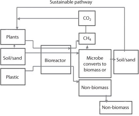
Figure 10.29 Sustainable pathwayfor material substance in the environment.
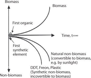
Figure 10.30 Synthetic non-biomassthat cannot be converted into biomass will accumulate far faster thannaturally-sourced non-biomass, which can potentially always be converted into biomass.
In evaluating equation (4.12), it is desirable to know all of the contents of the inflow matter. However, it is highly unlikely to know all the contents, even at a macroscopic level. In absence of a technology that would find the detailed content, it is important to know the pathway of the process to have an idea of the source of impurities. For instance, if de-ionized water is used in a system, one would know that its composition would be affected by the process of de-ionization. Similar rules apply to products of organic sources, etc. If we consider the combustion reaction (coal, for instance) in a burner, the bulk output will likely to be CO2. However, this CO2 will be associated with a number of trace chemicals (impurities) depending upon the process it passes through. Because, equation (4.12) includes all known chemicals (e.g., from source, adsorption/desorption products, catalytic reaction products), it would be able to track matters in terms of CNB and NCNB products. Automatically, this analysis will lead to differentiation of CO2 in terms of the pathway and the composition of the environment which is the basic requirement of equation (4.11). According to equation (4.12), charcoal combustion in a burner made up of clay will release CO2 and natural impurities of charcoal and the materials from the burner itself. Similar phenomenon can be expected from a burner made up of nickel plated with an exhaust pipe made up of copper.
Anytime, CO2 is accompanied with CNB matter, it will be characterized as beneficial to the environment. This is shown in the positive slope of Figure 10.31. On the other hand, when CO2 is accompanied with NCNB matter, it will be considered to be harmful to the environment, as this is not readily acceptable by the eco-system. For instance, the exhaust of the Cu or Ni-plated burner (with catalysts) will include chemicals, e.g., nickel, copper from pipe, trace chemicals from catalysts, beside bulk CO2 because of adsorption/desorption, catalyst chemistry, etc. These trace chemicals fall under the category of NCNB and cannot be utilized by plants (negative slope from). This figure clearly shows that the upward slope case is sustainable as it makes an integral component of the eco-system. With the conventional mass balance approach, the bifurcation graph of would be incorrectly represented by a single graph that is incapable of discerning between the different qualities of CO2 because the information regarding the quality (trace chemicals) are lost in the balance equation.

Figure 10.31 Results from Carboncombustion in a natural reactor and an artificial.
10.6 Classification of CO2
Carbon dioxide is considered to be the major precursor for current global warming problems. The entire climate change hysteria is premised on the ‘vile of carbon dioxide’ as if CO2 is not a part of the ecosystem. This characterization is typical of New Science. The origin of this like of characterization goes back to Atomism5. Nobel Laureate Linus
Pauling – prizewinner both for Chemistry and Peace, transmuted his work into the notion that humanity could live better with itself, and with nature, through the widest possible use and/or ingestion of chemicals. Essentially, his position is that “chemicals are chemicals,” i.e., that knowledge of chemical structure discloses everything we need to know about physical matter, and that all chemical combinations sharing the same structure are identical regardless of how differently they may actually have been generated or existed in their current form (his1954 Nobel Prize in Chemistry was “for his research into the nature of the chemical bond and its application to the elucidation of the structure of complex substances.”). This approach essentially disconnects a chemical product from its historical pathway. Even though the role of pathways has been understood by many civilizations for centuries, systematic studies questioning the principle have only been a recent development. For instance, in matters of Vitamin C, this approach advanced the principle that, whether from a natural or synthetic source and irrespective of the pathway it travels, all vitamin C is the same. Whereas in 1995, Gale et al., reported that vitamin C supplements did not lower death rates among elderly people and may actually have increased the risks of dying. Moreover, carotene supplementation may do more harm than good for patients with lung cancer (Josefson 2003). Obviously, such a conclusion cannot be made if subjects were taking vitamin C from natural sources.
In fact, the practices of people who live the longest lives indicate that natural products do not have any negative impact on human health (Haile et al., 2006). It has been reported that patients being treated for cancer should avoid antioxidant supplements, including vitamin C, because cancer cells gobble up vitamin C faster than normal cells which might give greater protection from tumors (Agus et al. 1999). Antioxidants present in nature are known to act as anti-aging agents. Obviously these antioxidants are not the same as those synthetically manufactured. The previously used hypothesis, “chemicals are chemicals,” fails to distinguish between the characteristics of synthetic and natural vitamins and antioxidants. The impact of synthetic antioxidants and vitamin C in body metabolism would be different than that of natural sources.
Numerous other cases can be cited demonstrating that the pathway involved in producing the final product is of utmost importance. Some examples have recently been investigated by Islam and coworkers (Khan and Islam 2007; Islam et al., 2010; 2015; 2016; Khan and Islam, 2012, 2016). If the pathway is considered, it becomes clear that organic produce is not the same as non-organic produce, natural products are not the same as bioengineered products, natural pesticides are not the same as chemical pesticides, natural leather is not the same as synthetic plastic, natural fibers are not the same as synthetic fibers, natural wood is not the same as fiber-reinforced plastic, etc. However, it is the economics that drove scientists to by-pass this true science and focus on the most tangible aspects that would give the desired conclusions (Islam et al., 2018a). Once the entire history of materials is considered a different picture emerges. For instance, in addition to being the only ones that are good for the long term, natural products are also found to be extremely efficient and economically attractive. Numerous examples are given in Khan and Islam (2007) as well as Chhetri and Islam (2008), in which it is shown that natural materials are more effective than their synthetic counterparts, without any negative side-effect (and with positive impact). For instance, unlike synthetic hydrocarbons, bacteria easily degrades natural vegetable oils (AlDarbi et al. 2005). The application of wood ash to remove arsenic from aqueous streams is more effective than removing it by the use of any synthetic chemicals (Rahman et al. 2004; Wassiuddin et al. 2002).
10.6.1 Isotopic Characterization
At present, there is consensus regarding the rate of fossil fuel combustion, which should account for an annual increase in CO2 by four ppm. However, the observed increase is only about two ppm. This discrepancy is explained in various ways. It is said that some CO2 dissolves in seawater. In pre-industrial times, the CO2 concentration of air was in equilibrium with the CO2 concentration of surface seawater. As atmospheric CO2 has risen, the equilibrium has been perturbed, such that the “excess” of CO2 in air now drives a flux of CO2 into the sea in an effort to re-establish equilibrium. It is also stated that the removal of CO2 from the atmosphere is related to the growth of forests and grasslands worldwide. This latter conclusion leads to the paradox that there has been severe deforestation, also attributed to industrial activities. This is countered by asserting that the rate of growth of large masses of vegetation (mostly forests) is higher than that of deforestation. Of course, that poses the question, if forestation and vegetation is increasing, why is the CO2 concentration rising?
To a first approximation, about half the CO2 emitted by combustion remains in the atmosphere, about 35% dissolves in the oceans, and 15% is taken up by the increase in the biomass of forests. It is recognized that CO2 absorption has declined in the ocean and at the same time general vegetation has not been using CO2 from combustion activities, rejecting a bulk amount to the atmosphere, thus causing overall rise. In this section, carbon dioxide has also been classified based on the source from where it is emitted, the pathway it traveled, and age of the source from which it came. It has been reported that plants favor a lighter form of carbon dioxide for photosynthesis and discriminate against heavier isotopes of carbon decades ago (Farquhar et al. 1989). They introduced a formulation, in which carbon isotopic composition is reported in the delta notation relative to the V-PDB (Vienna Pee Dee Belemnite, see Libes, 1992 for details) standard. δ13C (pronounced “delta c thirteen”) is an isotopic signature, a measure of the ratio of stable isotopes 13C : 12C, reported in parts per thousand (per mil, ‰).
(10.26)

In Eq. 10.1, the standard is an established reference material. The value of δ13C varies in time as a function of productivity, the signature of the inorganic source, organic carbon burial and vegetation type. In essence, this term is a signature of the path traveled by a material or the time function. Biological processes preferentially take up the lower mass isotope through kinetic fractionation. Therefore, the fractionation itself becomes a measure of the quality of CO2. The following formulation is based on Farquhar et al. (1989) and was used by several researchers, who studied the kinetic fractionation process.
(10.27)

in which, Δ13 is the C isotope discrimination, δ13Cair is the carbon isotope ratio of atmospheric CO2 (–7.8 2030) and δ13Cplant is the measured δ13C value of leaf material.
Ever since the recognition that the past concentrations of atmospheric CO2 level (pCO2) is critical to plant metabolism and extent of photosynthesis, many research projects have been undertaken. These studies attempt to determine correlation between pCO2 with changes in carbon isotope fractionation (Δ13C) in C3 land plants6.
Figure 10.32 shows the amount of carbon isotope fractionation per change in pCO2 (S, ‰/ppmv) as a function of pCO2. Note the similarity among the three S-curves. Circles are plotted as the midpoint of the range of pCO2 tested for each study. This sensitivity can vary under varying thermal conditions. Previous studies have reported that photosynthesis and plant enzyme activity can be strongly inhibited when grown at temperatures below 5C (Graham and Patterson, 1982; Ramalho et al., 2003). Some woody plants cannot withstand much below –6 C for any length of time and cease growth if the maximum daily temperature is below 9 C (Parker, 1963). For these low temperature conditions, thermal effects become the dominant limiting factors. Xu et al. (2015) reported variation in Δ13 with changing temperature. They observed a strong impact of mean annual temperature (MAT) on Δ13 in two mountain regions. MAT together with soil water content (SWC) in total accounted for a large proportion of the variation in Δ13 of the two mountainous regions. They observed that the impact of soil water availability on carbon isotope discrimination was limited for lower temperature values.
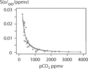
Figure 10.32 The effect of pCO2 on C3land plant carbon isotope fractionation based on field and chamber experimentson a wide range of C3 land plant species (from Cui and Schubert, 2016).
In (Equation 10.2), the fractionation process is controlled by the diffusion of CO2 through the stomata (Craig 1953) as well as CO2 fixation by ribulose bisphosphate carboxylase/oxygenase (RuBisCO; Farquhar and Richards 1984). These processes are highly sensitive to particulates of heavy metals as well as synthetic chemicals.
Hartman and Danin (2010) reported strong correlation between dry season green plants and rainfall – attributed to the combined product of ground water availability, evaporative demand, and improved water use efficiency (unique to desert shrubs and trees). Escudero et al. (2008) demonstrated that long-lived leaves from lignified species have higher δ13C values than short-lived leaves, due to reduced transpiration. They argued that this adaptation was designed to combat seasonal and annual shortages of water by minimizing the risk of leaf desiccation. Few studies have been available on how this process is altered in presence of anthropogenic CO2.
Fardusi et al. (2016) conducted meta-analysis with large amount of data. They con-cuded that the relationship between 13C and growth is better characterized at juvenile stages, under near-optimal and controlled conditions, and by analyzing 13C in leaves rather than in wood. Carbon isotope composition (13C) in plant tissues offers an integrated measure of the ratio between chloroplastic and atmospheric CO2 concentrations (Cc/Ca), and hence can be used to estimate the ratio between net CO2 assimilation rate (A) and stomatal conductance for water vapour, i.e., intrinsic water-use efficiency (WUEi) after making certain assumptions about mesophyll conductance and post-photosynthetic fractionations (Farquhar et al., 1984). Note that during an adaptation cycle – a term widely used by the scientific community since 1990s – plants and vegetations are likely to develop special water use efficiency skills in response to the surge of “toxic”7 CO2.
In this process, photosynthesis activities are enhanced in presence of higher WUEi. However, if higher WUEi implies a tighter stomatal control, it tends to be inversely correlated with growth (Brendel et al., 2002).
Intuitively, natural CO2 and anthropogenic CO2 should not behave the same way, mainly because anthropogenic CO2 is contaminated with various chemicals that are not found naturally. However, it is a topic that has eluded mainstream researchers. Few studies have been carried out to see how these two source affect long-term behaviour of CO2. Warwick and Ruppert (2016) attempted to document the relationships between the carbon and oxygen isotope signatures of coal and signatures of the CO2 produced from laboratory coal combustion in atmospheric conditions. This study unravelled some of the important justifications behind the intuitive assertion that natural materials cannot be the source of global warming. In their study, they took six coal samples from various geologic ages (Carboniferous to Tertiary) and coal ranks (lignite to bituminous). Duplicate splits of the six coal samples were ignited and partially combusted in the laboratory at atmospheric conditions. The resulting coal-combustion gases were collected and the molecular composition of the collected gases and isotopic analyses of δ13C of CO2, δ13C of CH4, and δ18O of CO2 were analysed by a commercial laboratory. Splits (~1 g) of the un-combusted dried ground coal samples were analyzed for δ13C and δ18O by the U.S. Geological Survey Reston Stable Isotope Laboratory. They reported that The the isotopic signatures of δ13CV-PDB (relative to the V-PDB standard) of CO2 resulting from coal combustion are similar to the δ13CV-PDB signature of the bulk coal (– 28.46 to – 23.86 ‰) and are not similar to atmospheric δ13CVPDB of CO2 (~ — 8 ‰). The δ18O values of bulk coal are strongly correlated to the coal dry ash yields and appear to have little or no influence on the δ18O values of CO2 resulting from coal combustion in open atmospheric conditions. There is a wide range of δ13C values of coal reported in the literature and the δ13C values from this study generally follow reported ranges for higher plants over geologic time. The values of δ18O relative to Vienna.
Standard Mean Ocean Water, VSMOW8) of CO2 derived from atmospheric combustion of coal and other high-carbon fuels (peat and coal) range from + 19.03 to+27.03‰ and are similar to atmospheric oxygen δ18OVSMOW values which average + 23.8‰. For reference, note that the isotopic ratios of VSMOW water are defined as follows:
- 2H/1H = 155.76 ± 0.1 ppm (a ratio of 1 part per approximately 6420 parts)
- 3H/1 hr = 1.85 ± 0.36×10⁻¹¹ ppm (a ratio of 1 part per approximately 5.41 × 10¹⁶ parts)
- 18O/16O = 2005.20 ± 0.43 ppm (a ratio of 1 part per approximately 498.7 parts)
- 17O/16O = 379.9 ± 1.6 ppm (a ratio of 1 part per approximately 2632 parts)
Figure 10.33 shows results from Warwick and Ruppert (2016). As can be seen from this figure, the δ13CVPDB of the coal combustion CO2 ranged from – 26.94 to – 24.16‰. Figure 10.34 shows results as reported by Warwick and Ruppert (2016). In this figure, the value of oxygen isotopic signature of atmospheric CO2 (δ18OVSMOW =+23.88) is from Brand et al. (2014). Run 1 (R1) and Run 2 (R2) are from Warwick and Ruppert (2016). shows those for δ18OVSMOW of CO2 ranged from + 19.03 to+27.03‰. In this experiment, two runs were conducted (Runs 1 and 2). The CO2 gases collected during the second combustion run had slightly heavier values of δ13CVPDB and lighter values of δ18OVSMOW. Eight coal combustion gases (three from Run 1, and five from Run 2) produced sufficient quantities of CH4 for the measurement of δ13CVPDB of CH4, and these values ranged from – 33.62‰ to – 16.95‰. Two of the collected gas samples from Run two yielded δ2HVSMOW-CH4 values of – 243‰ and – 239.8‰.
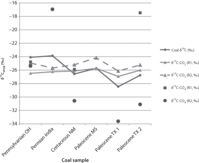
Figure 10.33 Plot of the isotopic signatures of δ13CVPDB for the original coal samples and carbon dioxide (CO2) and methane (CH4) of the gases derived from coal sample combustion (From Warwick and Ruppert, 2016).
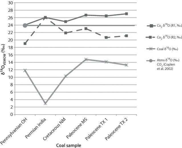
Figure 10.34 Plot of the isotopic signatures of δ18OVPDB forthe original coal samples and carbon dioxide (CO2)derived from coal sample combustion (From Warwick and Ruppert, 2016).
Figure 10.35 compares δ13CV-PDP values from effluents of a combustion in presence of atmospheric gases with combustion effluents in presence of high-purity combustion (brown squares in, as reported by Schumacher et al., 2011). The gases collected from the duplicate combustion runs indicate that the analytical results are generally reproducible. Schumacher et al. (2011) combusted samples of various organic materials (leaves, wood, peat, and coal) using controlled combustion temperatures (range 450 to 750 C) in the laboratory to study the effects of fuel type, fuel particle size, combustion temperature, oxygen availability, and fuel water content on the δ18O values of the produced CO2. The samples were combusted in high-purity oxygen with an isotopic signature of δ18O =+27.2‰; however, to compare the results to those from atmospheric combustion, two samples (a charcoal and a peat) were combusted using laboratory atmosphere (brown squares on right side of). Schumacher et al. (2011) described the influences on carbon and oxygen isotopic fractionation during the combustion process and reported the major influences on the isotopic composition of combustion gases include the temperature of combustion, the carbon isotopic signature of the combusted fuel material, fuel particle size, and water content of the fuel material. Schumacher et al. (2011) also suggested the δ18O signature of the combusted organic material may influence the δ18O signature of the resulting combustion-derived CO2. While this is intuitively correct, they did not measure δ18O of the coal samples used in their study. Schumacher et al. (2011) chose to use high-purity oxygen for their combustion experiments because of the dampening effect of nitrogen and water vapor on the combustion process in natural atmosphere. Atmospheric components may also react with the combustion gases. The role of atmospheric gases in shaping the isotopic character of CO2 is confirmed in, which compares the two cases. It reveals that components otherwise not considered in conventional analysis (the ones we call ‘intangibles’) are the one made a difference in isotopic behavior of the two cases. Although preliminary, the results of our study may help to better characterize the oxygen and carbon isotopic character of CO2 derived from atmospheric coal combustion.
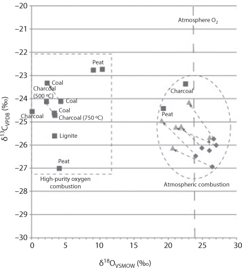
Figure 10.35 Plot of δ18OVSMOW SLAP ofCO2 derived from combustion of coal andother carbon-rich fuels and δ13CVPDB valuesof the combustion-derived CO2 (from Warwick and Ruppert, 2016).
Carbon has two isotopes, namely, 12C and 13C. Each has six protons in the nucleus of the atom, hence both are carbon. However, 13C has an extra neutron and thus a greater mass.
Adjacent atoms in molecules vibrate like balls attached to springs. In plain language, it means, in presence of an isotope, neighbouring atoms are more susceptible to interactions with the isotope. Lighter atoms vibrate more rapidly, and atoms vibrating more rapidly are easier to separate. Hence light atoms react more rapidly than heavy atoms in chemical and biochemical processes. In general, it is known that plant materials have less of the heavy isotope, 13C, than CO2 from which it is produced, in essence plants fractionate and accumulate 13C, which then get transferred to animals that eat them. Fossil fuels of biogenic origin would have the same feature. The addition of organic carbon to air causes the resulting CO2 mixture to have less 13C. So, for example, at night, the 13C/12C ratio of CO2 in air decreases as plant material decays, and as fossil fuel CO2 is added in populated areas. Similarly, in winter, the 13C/12C ratio of CO2 in air again decreases as vegetation slowly rots. The 13C/12C ratio of CO2 is presented as δ13C, which is the difference, in parts per thousand (tenths of a percent) between the 13C/12C ratio of a sample and a reference gas.
The δ13C signature of bulk coal has been well studied and reported in the literature (Singh et al., 2012). Gröcke (2002) has compared the carbon isotope composition of ancient atmospheric CO2 to that of organic matter derived from higher-plants and suggested that both vary over geologic time. This observation confirms that CO2 is part of the organic cycle and as such should not create imbalance in the ecosystem. Carbon isotope ratios in higher-plant organic matter (δ13Cplant) have been shown in several studies to be closely related to the carbon isotope composition of the ocean– atmosphere carbon reservoir, the isotopic composition of CO2 being a reliable tracer. These studies have primarily been focused on geological intervals in which major perturbations occur in the oceanic carbon reservoir, as documented in organic carbon and carbonates phases (e.g., Permian–Triassic and Triassic–Jurassic boundary, Early Toarcian, Early Aptian, Cenomanian–Turonian boundary, Palaeocene–Eocene Thermal Maximum (PETM)). All of these events, excluding the Cenomanian–Turonian boundary, record negative carbon isotope excursions, and many authors have postulated that the cause of such excursions is the massive release of continental margin marine gas-hydrate reservoirs. That itself brings in Methane into the picture. In general a very negative carbon isotope composition (δ13C, around –60%%) is reported in comparison with higher-plant and marine organic matter, and carbonate. The residence time of methane in the ocean– atmosphere reservoir is short (around 10 years) and is rapidly oxidized to CO2, causing the isotopic composition of CO2 to become more negative from its assumed background value (δ13C of about –7‰). Such rapid negative δ13C excursions can be explained with geological events. Notwithstanding this, the isotopic analysis of higher-plant organic matter (e.g., charcoal, wood, leaves, pollen) has the ability to (i) record the isotopic composition of palaeoatmospheric CO2 in the geological record, (ii) correlate marine and non-marine stratigraphic successions, and (iii) confirm that oceanic carbon perturbations are not purely oceanographic in their extent and affect the entire ocean–atmosphere system (Grocke, 2002). The problem is, there are case studies that show that the carbon isotope composition of palaeoatmospheric CO2 during the Mid-Cretaceous had a background value of –3‰, but fluctuated rapidly to more positive (around + 0.5‰) and negative values (around –10‰) during carbon cycle perturbations (e.g., carbon burial events, carbonate platform drowning, large igneous province formation). As such, fluctuations in the carbon isotope composition of palaeoatmospheric CO2 would compromise our use of palaeo-CO2 proxies that are dependent on constant carbon isotope ratios of CO2 (Grocke, 2002). Terrestrial plants can be divided into three groups on the basis of distinctions in photosynthesis and anatomy, namely:
- C3 (Calvin–Bensen cycle, temperate shrubs, trees and some grasses, see Figure 10.36);
- C4 (Hatch–Slack cycle, herbaceous tropical, arid-adapted grasses); and
- Crassulacean acid metabolism (CAM, succulents).
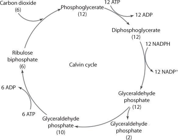
Figure 10.36 A simplified version of the C3 Calvin cycle (From Grocke, 2002).
Figure 10.36 Is a depiction of the Calvin cycle. Note that the Calvin cycle (also known as the Benson-Calvin cycle) is the set of chemical reactions that take place in chloroplasts during photosynthesis. The cycle is light-independent in the sense that it takes place after light energy has been captured during photosynthesis. represents six turns of the cycle, each turn of the cycle representing the use of one molecule of CO2. Adenosine triphosphate (ATP) and nicotinamide adenine dinucleotide phosphate (NADPH, which is a reduced form of NADP+) are the products of the light-dependent reactions, which drive the Calvin cycle (ADP denotes adenosine diphosphate). The brackets after each element represent the number of molecules produced.
It has been suggested that C4 plants were present in the geological record prior to the Miocene (Ehleringer et al. 1991). Evans et al. (1986) conducted experiments on the isotopic composition of CO2 before and after it passed through the leaves of a C3 plant and it was found that 12CO2 was preferentially incorporated into the leaf, although if 12CO2 concentrations were low, then relatively more 13CO2 was incorporated into the leaf. Subsequently, it was shown that C3 and C4 plant groups have isotopically distinct δ13Cplant ranges: C3 plants range between –23 and –34%% with an average of –27%%, whereas C4 plants range between –8 and –16%% with an average of –13%% (Vogel 1993). Hence, the carbon isotope composition of ancient higher-plant organic matter, excluding environmental effects should provide researchers with a proxy for discriminating between these two main plant groups in the geological record. Similarly, such distinction can be made between CO2 from fossil fuel and CO2 from refined oil (e.g., gasoline). The fact that refining process adds many artificial chemicals, the Calvin cycle is affected. Figure 10.37 shows how the Calvin cycle can act as a fractionation column. In this figure, the term Σcontaminants is the collection of all contaminant molecules that come from artificial components (the ones termed ‘intangible’ by Khan and Islam, 2016). It includes the entire history of a particle/molecule. For instance, if CO2 came from plants that itself used pesticide and chemical fertilizer, this term will contain intangible amounts of the chemicals used in those processes. In the first phase, there will be components that will be rejected (Reject0) even before entering the Calvin cycle. It is similar to rejection or fractionation of 13CO2 molecules. This process of elimination continues at various stages, each corresponding to Rejecti, where i is the number of the cycle.
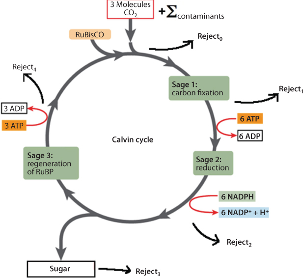
Figure 10.37 The CO2 rejects due to contaminants.
Table 10.8 Shows δ18O of coal results represent the average of two analyses as reported by Warwick and Ruppert (2016). The isotopic results of the δ13CV-PDE of the coal combustion CO2 ranged from –26.94 to –24.16‰ and those for δ18OV-SMOW of CO2 ranged from +19.03 to + 27.03‰. The CO2 gases collected during the second combustion run had slightly heavier values of δ13CV-PDB and lighter values of δ18OV-SMOW. Eight coal combustion gases produced sufficient quantities of CH4 for the measurement of δ13CVPDB of CH4, and these values ranged from –33.62‰ to –16.95‰. The coal combustion-derived δ13CVPDB-CO2 signatures were found to be similar to that of the δ13CVPDB of the bulk coal (–28.46 to –23.86‰) and are not similar to modern atmospheric δ13CVPDB of CO2 (–8.2 to –6.7‰; as reported by Coplen et al., 2002). The values of δ18OVSMOW of CO2 (+19.03 to + 27.03‰) from the coal combustion gases from this study are similar to atmospheric oxygen δ18O values which average + 23.8‰ (Coplen et al., 2002). There is a wide range of δ13CV-PDB values of coal reported in the literature and the values obtained by Warwick and Rupert (2016) generally follow previously reported ranges for higher plants over geologic time. The isotopic signatures of δ13CVPDB of CO2 resulting from laboratory coal partial combustion are similar to and probably derived from the original δ13C signatures of the coal. The δ18OVSMOW values of coal show a strong correlation to the coal dry ash yields and appeared to have little or no influence on the δ18OVSMOW values of CO2 resulting from coal combustion. Coal burning is similar to crude oil burning. However, the same conclusion would not apply to refined oil burning and irrespective of the isotopic composition of the combustion products, the effect on the ecosystem will be long-lasting and irreversible. Warwick and Ruppert (2016) emphasized the need to develop better techniques for characterizing CO2 which results from the combustion of coal.
Table 10.8 Carbon and Oxygen Isotope Compositions in Bulk Coal and Gases Collected From Combusted Coal, All Isotopic Values Given in Per Mil (‰). (From Warwick et al. 2016).
| Sample | Sample number |
Run |
Bulk coal |
Collected gases from partially combusted coal |
||||||
δi3Cvpob |
Mass fraction of C (%) |
δ1SOvSMOW |
Mass fraction of 0 (%) |
CO2 |
CH4 |
|||||
δ13Cvpdb |
δ1S0vsmow |
Δ13Cvpdb |
62Hvsmow |
|||||||
| Pennsylvanian OH | E-0709002–063 | 1 | — 26,57 |
54.6 |
10,29 |
15.5 |
–26.13 |
24.93 |
–25.89 |
na |
| Pennsylvanian OH | E-0709002–063–2 | 2 | –25.2 |
21.89 |
–30.57 |
na |
||||
| Permian India | SBT-19-R7 | 1 | –23.86 |
48 |
2.96 |
9.2 |
–26.24 |
26.04 |
na |
na |
| Permian India | SBT-19-R7–2 | 2 | –25.68 |
26.05 |
–16.95 |
na |
||||
| Cretaceous NM | 07018–01314GBC | 1 | –24,09 |
69.4 |
11,82 |
11.3 |
–26.48 |
24.03 |
–24.78 |
na |
| Cretaceous NM | 0701S-01314GBC- 2 | 2 | –24.95 |
19.03 |
–25.39 |
na |
||||
| Paleocene MS | MS-02-DU | 1 | –25.73 |
42 |
14.77 |
25.5 |
–25.74 |
26.67 |
na |
na |
| Paleocene MS | MS-02-DU-2 | 2 | –2416 |
23.04 |
na |
na |
||||
| Paleocene TX1 | PA-2-CN6 | 1 | –28,46 |
62.7 |
14,12 |
21.4 |
–26.94 |
26.46 |
na |
na |
| Paleocene IX 1 | PA-2-CN6–2 | 2 | –26.13 |
20.65 |
–33.62 |
–239.8 |
||||
| Paleocene TX 2 | PA-2-CN2 | 1 | –26.77 |
59.7 |
13.27 |
21 |
–26.01 |
27.03 |
–17.46 |
na |
| Paleocene TX 2 | PA-2-CN2-2 | 2 | –25.23 |
21.12 |
–31.11 |
–243 |
||||
Coplen et al. (2002) compiled a report on isotopic composition of a number of naturally occurring materials. The principal elements studied are reported in Table 10.9. Their report is a useful listing of major players of global warming.
Table 10.9 The Minimum and Maximum Concentrations of a Selected Isotope in Naturally Occurring Terrestrial Materials (From Coplen et al., 2002).
| Isotope | Minimum mole fraction |
Maximum mole fraction |
||
| 2H | 0 |
.000 0255 |
0 |
.000 1838 |
| 7Li | 0 |
.9227 |
0 |
.9278 |
| 11B | 0 |
.7961 |
0 |
.8107 |
| 13C | 0 |
.009 629 |
0 |
.011 466 |
| 15N | 0 |
.003 462 |
0 |
.004 210 |
| 18O | 0 |
.001 875 |
0 |
.002 218 |
| 26Mg | 0 |
.1099 |
0 |
.1103 |
| 30Si | 0 |
.030 816 |
0 |
.031 023 |
| 34S | 0 |
.0398 |
0 |
.0473 |
| 37Cl | 0 |
.240 77 |
0 |
.243 56 |
| 44Ca | 0 |
.020 82 |
0 |
.020 92 |
| 53Cr | 0 |
.095 01 |
0 |
.095 53 |
| 56Fe | 0 |
.917 42 |
0 |
.917 60 |
| 65Cu | 0 |
.3066 |
0 |
.3102 |
| 205Tl | 0 |
.704 72 |
0 |
.705 06 |
10.6.2 Isotopic Features of Naturally Occurring Chemicals
Coplen et al. (2002) documented isotopic features of a number of chemicals that related to global warming and climate change. Following discussion relies on their report.
Carbon monoxide (CO): In nature, oxidation of methane or other hydrocarbon can lead to the formation of carbon monoxide. This is inherent to fossil fuel burning. Also, biomass burning (including during forest fires), transportation, industry, heating, oceans, and vegetation, they will all generate certain volume of CO. The primary sinks of atmospheric methane are oxidation by the hydroxyl radical (OH) and uptake by soils. Its average residence time in the atmosphere is about 2 months. The values of δ13C of CO in the atmosphere in Antarctica (where the atmosphere is unpolluted) range between –31.5 ‰ and –22 ‰.
Organic carbon: Organic carbon is the essence of vegetation and as such the driver of life on earth. Any biological assimilation of carbon by plants results in depletion of 13C in the organism’s tissues relative to the carbon sources (CO2 and HCO3 −). The magnitude of the 13C depletion depends on the species and the carbon fixation pathways utilized, environmental factors such as temperature, CO2 availability, light intensity, pH of water, humidity, water availability, nutrient supply, salinity, cell density, age of photosynthesizing tissue, and oxygen concentration. Based on our presentation in Chapter 4, such speciation will also depend on any artificial chemical that has been added to the pathway (e.g., pesticide, chemical fertilizer, refining catalyst). Plants assimilate carbon using two different pathways, which leads to a classification of three photosynthetic groups. The predominant fixation reaction is carboxylation of ribulo-sebisphosphate (RuBP) to the C3-product phosphoglycerate, which generally results in δ13C of plants between –35 ‰ and –21 ‰, but as low as –35 ‰. C3 plants tend to grow in cool, moist, shaded areas and comprise 80 to 90 percent of plants. All trees, most shrubs, some grasses from temperate regions and tropical forests, and common crops such as wheat, rice, oats, rye, sweet potatoes, beans, and tubers utilize the C3 pathway. The second reaction involves the carboxylation of phosphoenolpyruvate to the C4 product oxalacetic acid. This fixation is more efficient leading to less depletion in 13C; the δ13C of C4 plants ranges between –16 ‰ and –9 ‰. C4 plants, such as maize, sugar cane, sorghum, and grasses in Australia, Africa, and other subtropical, savannah, and arid regions, tend to grow in hot, dry, sunny environments. Animals and microbial heterotrophs generally have δ13C values within 2 ‰ of their food supply. A wider range is possible for various organs and tissues within a single organism can have a wider range. It is the case because each organic part acts as a natural partitioning agent. The δ13C values of fresh tissues and the collagen and hydroxyapatite from bones and teeth have been applied to food web studies and reconstructions of prehistoric diet and vegetation patterns. For example, geographic variations of the δ13C values of hair in humans compares favorably with the 13C depleted diets of Germans (δ13C = –23.6 ‰), the seafood and corn diets of Japanese (δ13C = –21.2 ‰), and the corn diets of Americans (δ13C = –18.1 ‰), as reported by Nakamura et al. (1982). Isotope-ratio analyses of organisms found in the literature primarily have been confined to analysis of molecules or whole tissues. Brenna (2001) correctly pointed out that physiological history is retained in natural isotopic variability.
Brenna (2001) suggested that a strong case that future studies of physiological isotope fractionation should involve position-specific isotope analysis and should reveal the relationship of diet and environment to observed isotope ratio. The δ13C value of sedimentary organic matter is affected by the local flora and fauna, the environmental conditions, secondary processes, recycling of older carbon-bearing sediments, and anthropogenic wastes. At this juncture, few studies have been reported on the role of anthropogenic wastes and their role in altering natural degradation. During diagenesis, the biopolymers of newly deposited sediments are biochemically degraded by microorganisms. Most of the organic matter is oxidized to CO2 and H2O or reused as biomolecules within living organisms. Within limited settings, terrestrial plant sediments tend to be more depleted in 13C than marine plankton sediments. For example, river sediments, with an average δ13C value of about –26 ‰, tend to become enriched in 13C at the river mouth, presumably because of increasing amounts of marine plankton (as opposed to terrestrial C3 plant) input (Deines, 1980). This can explain the nature of CO2 absorption in the ocean that shows decline in the presence of surplus anthropogenic CO2.
Elemental carbon: As organic matter undergoes burial and thermal alteration, functional groups of organic compounds are lost, H2O and CO2 are produced, and methane is evolved. This process is simulated in a laboratory as pyrolysis. In a natural setting, the final product of this reduction is graphite, with δ13C ranging between –41 ‰ and +6.2 ‰. It appears that diamonds conform to this range with δ13C ranging between –15.6 ‰ to –4.4 ‰, in line with depth-related variations in the mantle.
Ethane: Low temperature serpentinization of ophiolitic rocks generates free hydrogen along with minor amounts of methane and ethane. Studies indicate that the δ13C values of ethane as high as –11.4 ‰. Gases in the potash layers are highly enriched in 13C with δ13C values as positive as +6.6 ‰. The mode of formation is still uncertain although hypotheses include (1) maturation of organic matter rich in 13C; (2) transformation of CO2 enriched in 13C to CH4; (3) unknown bacterial isotope fractionation; and (4) abiotic gas formation during halokinesis (including salt tectonics). The most negative δ13C found in the literature for a bacterially formed ethane is –55 ‰. This finding confirms the role of microorganisms in reducing isotopic fractions.
Methane: The two major methane production processes are: (1) diagenesis of organic matter by bacterial processes; and (2) thermal maturation of organic matter. Biogenic methane follows one of two major pathways for biogenic methane production: (1) CO2 reduction, which dominates in marine environments; and (2) acetate fermentation, which dominates in fresh-water environments. The δ13C values of marine methane range from –109 ‰ to 0 ‰, whereas methane in freshwater sediments and swamps is more enriched in 13C, but have a smaller range in carbon isotopic composition, with δ13C values range from –86 ‰ to –50 ‰. The isotopic compositions of thermogenic methane are affected by the geological history of the basins and they depend on such factors as the extent of conversion of organic matter and the timing of gas expulsion, migration, and trapping.
The δ13C of thermogenic methane that is associated with natural gas ranges from –74 ‰ to +12.7 ‰. The reason behind such positive δ13C is unknown but is indicative of the fact that kinetic of higher temperature is complex. Methane is an important atmospheric greenhouse gas with major natural and anthropogenic sources including swamps, rice paddies, ruminants, termites, landfills, fossil-fuel production, and bio-mass burning. The δ13C of atmospheric methane is relatively constant, generally ranging between –50.58 ‰ and –46.44 ‰.
Nitrogen: Although nitrogen is about twenty-fifth in crustal abundance, it comprises 78.1 percent of the atmosphere by volume. A primary use of nitrogen gas is as an inert atmosphere in iron and steel production and in the chemical and metallurgical industry. Large quantities of nitrogen are used in fertilizers and chemical products. More moles of anhydrous ammonia are produced worldwide than any other nitrogen-bearing compound. This ammonia is distinctly different from natural ammonia that is a common waste among living organisms. The natural abundance of stable isotopes of elements in animal tissue is influenced by both biotic and abiotic factors. Biotically, animals feeding at higher trophic levels are enriched in the ratio of 15N:14N (15N) relative to their food resources owing to the preferential excretion of 14N. Abiotically, increases in 15N may also reflect different sources of biologically available nitrogen, including nitrogen resulting from denitrification of chemical fertilizer. In Chapter 4, we discussed how chemical fertilizer would alter the overall nitrogen cycle, thereby contributing to imbalance in the ecosystem. Lake et al. (2011) variation in 15N among freshwater turtle populations to assess spatial variation in 15N and to determine whether this variation can be attributed to differences in nitrogen source or trophic enrichment. They examined nitrogen and carbon stable isotope ratios in duckweed (genus Lemna L.) and in Painted Turtles (Chrysemys picta) in aquatic ecosystems expected to be differentially affected by agricultural activity and denitrification of inorganic fertilizer. Across sites, C. picta δ15N was strongly correlated with Lemna 15N and was elevated in sites influenced by agricultural activity. Furthermore, trophic position of turtles was not associated with δ15N but was consistent with expected values for primary consumers in freshwater systems, indicating that differences in tissue δ15N could be attributed to differences in initial sources of nitrogen in each ecosystem. In all cases, δ15N was the lowest in absence of agricultural activities using chemical fertilizers.
Since fossil fuel refining involves the use of various toxic additives, the carbon dioxide emitted from these fuels is contaminated and is not favored by plants. If the CO2 comes from wood burning, which has no chemical additives, this CO2 will be more favored by plants. This is because the pathway the fuel travels, from refinery to combustion devices, makes the refined product inherently toxic (Islam et al., 2010). The CO2 that the plants do not synthesize accumulates in the atmosphere. The accumulation of this rejected CO2 must be accounted for in order to assess the impact of human activities on global warming. This analysis provides a basis for discerning between natural CO2 and ‘toxic’ CO2, which could be correlated with global warming.
10.6.3 Photosynthesis
For the ecosystem and sustainability of nature, photosynthesis is the most crucial occurrence. In term, the fact that photosynthesis occurs at visible wavelengths is of utmost interest. Any skewing of the light spectrum will have implication on photosynthesis. Chlorophyll a (C55H70O6N4Mg) and chlorophyll b (C55H70O6N4Mg) play major role in the absorption of solar energy for the sake of photochemical reactions of photosynthesis (Murray et al., 1986). In plants, it is the pigment chlorophyll a that is responsible for absorbing incoming solar radiation at selected wavelengths, and performing charge separation to gather electrons from an electron donor, such as H2S or H2O. While New Science presents these ‘electrons’ as uniform, homogenous, rigid entitities that cannot be affected by the presence of contaminants, Islam (2014) demonstrated that by using the galaxy model (see previous chapters), one can show that the presence of tiniest amoung of contaminants, one can affect the overall chemical reaction. The range of the spectrum, for which oxygenic photosynthesis occurs is largely restricted to the 400–700 nm range, called “photosynthetically active radiation” (Shields et al., 2016). The term, “Photosynthetically active radiation” (PAR) represents the spectral range of solar radiation from 400 to 700 nanometers, which is amenable to processing by photosynthetic organisms. Islam (2014) showed that this range is not a matter of artificially simulating the light component, it must have the same natural components, present in sunlight. Such conclusion cannot be reached using conventional Atomic theory. Certain organism, such as such as cyanobacteria, purple bacteria, and heliobacteria, can exploit solar light in slightly extended spectral regions, such as the near-infrared. While they are part of the overall ecosystem and necessary for total balance, the most important components are within the visible light region. As we have seen in previous chapters, Chlorophyll is the most abundant plant pigment, is most efficient in capturing red and blue light. Accessory pigments such as carotenes and xanthophylls harvest some green light and pass it on to the photosynthetic process, but enough of the green wavelengths are reflected to give leaves their characteristic color, green being the widest of the spectrum of visible lights. Even when chlorophyll is degraded during autumn (because it contains N and Mg), it remains essential to plants and remain in the leaf producing red, yellow and orange leaves. Chlorophyll a uses this PAR and cannot thrive in presence of contaminants. One the other hand, Chlorophyll b, which support activities of Chlorophyll a, is far less sensitive to contaminants. As shown in Chlorophyll a absorbs energy from wavelengths of blue-violet and orange-red light while chlorophyll b absorbs energy from wavelengths of green light. The characteristic wavelength for Chlorophyll a is 675 nm while for chlorophyll b it is 640 nm. It is known that higher plants and green algae contain chlorophyll a and chlorophyll b in the approximate ratio of 3:1. Chlorophyll c is found together with chlorophyll a in many types of marine algae. While, red algae (Radophyta) contain principally chlorophyll a and also chlorophyll d. α - carotene occurs always together with chlorophylls (Edarous, 2011). Chlorophyll are structurally originated from methyl phytolesters of dicarboxylic acid that consists of prophyrin head with four rings centrally linked to magnesium atoms and a phytol tail (C20H39OH) with long aliphatic chain of alcohol. The following distinctions between the two types of chlorophylls can be made.
- Chlorophyll b is more absorbent while chlorophyll a is not.
- Chlorophyll a is the reaction center of the antenna array of core proteins while chlorophyll b regulates the size of the antenna. It offers abundant energy to carry out the reactions of photosynthesis.
- Specifically, Chlorophyll a (and other accessory pigments that vary by organism) absorbs strongly in the blue and also in the red region of the visible spectrum (Figure 10.38). The lower absorption coefficient in the green range of the spectrum is responsible for the higher reflectance of plants in this range, and their resulting green appearance to the human eye.
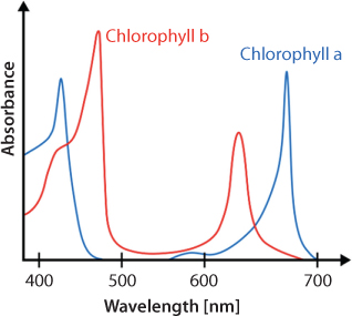
Figure 10.38 Light spectrum for Chlorophyll a and Chlorophyll b.
Figure 10.39 shows the absorption spectrum, as well as the action spectrum and quantum yield for chlorophyll while engaged in the process of oxygenic photosynthesis. Note the drop in the absorption coefficient in the green range of the spectrum (495–570 nm), and the sharp drop at ~700 nm.

Figure 10.39 Absorption spectrum and quantum yield vs. wavelength (From Gale and Wandel).
Chlorophyll b: Magnesium [methyl (3S,4S,21R)-14-ethyl-13-formyl-4,8,18-trimethyl-20-oxo-3-(3-oxo-3-{[(2E,7R,11R)-3,7,11,15-tetramethyl-2-hexadecen-1-yl]oxy}propyl)-9-vinyl-21-phorbinecarboxylatato(2-)-κ2N,N’]
Structural compositions of Chlorophyll a and b are shown in Figure 10.40. Each of these is vulnerable to toxic chemicals that are added through chemical fertilizer or pesticides (Turkilmaz and Esiz, 2015; El-Aswed et al., 2008). Whereas, the loss of chlorophyll in response to aging resulting in natural senescence is an inevitable process in plant development, heavy metals or the presence of unusal isotopic concentration can accelerate the ageing effects. El-Said Salem (2016) identified following organic activities that are affected by chemical pollutants.
- Formation of plastids; the small dense protoplasmic inclusion in the cell plant, and may act as a special centers of chemical activity. These plastids when exposed to light become pigmented and become chloroplasts. The presence of pollutants, even in intangible form (not detectable with conventional analytical tools) can alter plastid compositions.
- Transformation of plastids to chloroplasts (in plastid containing chlorophyll, with or without other pigments embedded singly or in consider numbers in the cytoplasm of a plant cell. In this process, pesticides may interfere with the formation of plastids or chloroplasts.
- Inhibition of pigments synthesis due to the accumulation of the carotenoids precursor phytofluene and phytoene, and the loss of chlorophyll, carotenoids. Chloroplast ribosomes and grana structure such accumulation resulted from the blockage of dehydrogenation reactions in the biosynthesis of the carotenoids in herbicide – treated leaves.

Figure 10.40 Chlorophyll a and Chlorophyll b (molecular structure)Chlorophyll a: Magnesium [methyl (3S,4S,21R)-14-ethyl-4,8,13,18-tetramethyl-20-oxo-3-(3-oxo-3-{[(2E,7R,11R)-3,7,11,15-tetramethyl-2-hexadecen-1-yl]oxy}propyl)-9-vinyl-21-phorbinecarboxylatato(2-)-κ2N,N’].
In several studies, it was found that seed oil content (oil concentration) decreased or responded weakly to increase in N supply, due to the concomitant increase in heavier protein production under high N nutrition (Abbadi et al. 2008, Ghasemnezhad and Honermeier 2008). This could be a result of the competition between protein synthesis and fatty acid synthesis for carbon building blocks. Ghasemnezhad and Honermeier (2008) also suggested that fatty acid synthesis has higher carbo-hydrate requirement than protein. Consequently, the increased N supply would enhance protein synthesis at the expense of fatty acid synthesis for primrose seeds.
Young et al. (2010) studied how chemical fertilizers affect the photosynthesis process. In this study, leaf gas exchange measurements and leaf nitrogen content were determined for four varieties of J. curcas, grown in the field or in pots. Based on stable carbon isotope analysis (δ13C) and gas-exchange studies, they reported the range of leaf photosynthetic rates (or CO2 assimilation rates) to be typically between 7 and 25 μmol (CO2) m−2 s−1 and light saturation beyond 800 μmol(quanta) m−2 s−1.
10.6.4 The Effect on Carbon (114C and δ13C)
The isotopic composition of carbon in atmospheric CO2 in oceanic and terrestrial carbon reservoirs fluctuate naturally. However, the introduction of anthropogenic emissions after the ‘plastic revolution’ has created imbalance the intensity of the fluctuation has increased. Naturally, Carbon-14 (14C) is continually formed in nature by the interaction of neutrons with nitrogen-14 in the Earth’s atmosphere; the neutrons required for this reaction are produced by cosmic rays interacting with the atmosphere. Similar isotopes can be formed during testing of nuclear bombs, which was the case during 1950 s. On the other hand, in organic systems, the ratio of 13C and 12C isotopes fluctuates depending on the plant photosynthesis. Similarly, the 13C/12C ratio varies within sedimentary rock, leaving behind a signature, which can be used to characterize the rock.
Fossil fuel burning decreases the proportion of the isotopes 14C and 13C relative to 12C in atmospheric CO2 by the addition of aged, plant-derived carbon that is partly depleted in 13C and entirely depleted in 14C (Graven et al., 2017). This process is referred to as the Suess effect following the early observations of radiocarbon in tree rings by Hans Suess (Suess, 1955). Suess (1955) pointed out that a decrease in the specific C14 activity of wood at time of growth during the previous 50 years. The decrease amounted to about 3.4% percent in two trees from the east coast of the United States. A third tree, from Alaska, investigated at that time, showed a smaller effect. The decrease was attributed to the introduction of a certain amount of C14-free CO2 into the atmosphere by artificial coal and oil combustion and to the rate of isotopic exchange between atmospheric CO2 and the bicarbonate dissolved in the oceans. In order to obtain more quantitative data concerning the effect, mass-spectrometric C13 determinations were made and used to correct for isotope fractionation in nature and in the laboratory. For this purpose a few cubic centimeters of C2H2 of each sample were converted to CO2 by recycling over hot CuO and the mass-spectrometer measurements were made. Eleven samples of wood from four different trees, each sample consisting of a small range of annual rings, were investigated; for comparison, three samples of marine carbon were also measured. Two independent sets of counting equipment were used. Suess observed marked variations among samples, always in the direction of a lower C14 content. The tree from the east coast of the United States showed the largest effect. The smaller effects noted in the other three trees indicate relatively large local variations of CO2 in the atmosphere derived from industrial coal combustion, and that the world wide contamination of the earth’s atmosphere with artificial CO, probably amounts to less than 1%. Hence the rate by which this CO2 exchanges and is absorbed by the oceans was deemed to be greater than previously assumed. Carbon of marine origin is known to show a lower C14 content than expected when one assumes complete equilibration with the atmosphere. It is because in the atmosphere exchange with organic matter is far more intense and direct than in the ocean.
The term Suess effect was also later adopted for 13C (Keeling, 1979). The magnitudes of the atmospheric 14C and 13C Suess effects are determined not only by fossil fuel emissions but also by carbon exchanges with the ocean and terrestrial reservoirs and the residence time of carbon in these reservoirs, which regulate the mixing of the fossil fuel signal out of the atmosphere (Keeling, 1979). The first measurements of the δ13C of dissolved inorganic carbon (DIC) of ocean surface waters were made in 1970 (Kroopnick, 1974) and serve as a baseline for assessing how the carbon isotopic composition of the oceans have changed in response to the burning of fossil fuel CO2 over the last decades. However, in order to gain a longer and more complete picture of the marine δ13C Suess effect, Black et al. (2011) suggested the use of indirect measurements of changes in surface water δ13C, most notably those preserved in carbonate secreting marine organisms. Recently, Swart et al. (2010) presented a compilation of coral δ13C records from throughout the global ocean and estimated that the average rate of change in δ13C in all of the records between 1900 and 1990 was –0.01 ‰ yr−1. Black et al. (2011) reported previous findings that the anthropogenic-induced decrease in δ13C is 0.9 ‰ in the Arctic and 0.6 ‰ in both the eastern North Atlantic and the Southern Ocean. By combining data collected as part of the Cariaco Basin ocean time series study with data derived from a sediment core from the basin, Black et al. (2011) produced a annual record of δ13C in planktonic foraminiferal for the southern Caribbean for the last 300 years.
Figure 10.41 a shows pCO2 Mauna Loa atmospheric and Cariaco Basin water cases. Changes in Cariaco Basin pCO2 appear to be reflecting large scale changes in atmospheric CO2, rather than just local processes. In absence of direct measurements of the δ13C of surface water to asses how this increase in pCO2 over the previous 15 years is manifested as a change in the carbon isotopic composition of Cariaco Basin surface waters, Black et al. (2011) used the δ13C of planktonic foraminifera collected in sediment traps during this period as an indirect way of determining changes in surface water δ13C of dissolved inorganic carbon (DIC). Using this approach, they track back to 1700 by coupling the sediment trap results with a foraminiferal δ13C record derived from Cariaco Basin sediment cores. As shown in Figure 10.41 (b), by directly comparing coincident carbon isotope data for both sediment trap and box core samples for the period from 1996 through 2007, they could assess the fidelity of the G. ruber δ13C record preserved in the sediments. For this period of overlap the two G. ruber results indicate that the initial isotopic signature has not undergone postdepositional alteration. Over this 12 year interval, the sediment trap δ13C record decreases from 1.19 ‰ to 0.86 ‰ (–0.03 ‰ yr−1), while the box core record decreases from 1.23 ‰ to 1.00 ‰ (–0.02 ‰ yr−1). For comparison, the Mauna Loa atmospheric δ13C record also has a rate of change of –0.03 ‰ yr−1 for this time period Figure 10.41 (b). This suggests that the Cariaco Basin G. ruber δ13C is not controlled primarily by local processes but rather can be used as a proxy for broad-scale changes in the δ13C of surface water DIC associated with ocean-atmosphere exchange of CO2.

Figure 10.41 (a) Comparison of atmospheric CO2 and d13C to Cariaco Basin sediment trap and sediment core d13C. Mauna Loa atmospheric pCO2 and Cariaco Basin water pCO2 between 1996 and 2009. For both cases, DCO2/Dt = 1.95 ppm/yr. (From Black et al., 2011).
Figure 10.42 shows that the atmospheric pCO2 increases slightly between the mid-1800s and 1950, after which pCO2 values abruptly rise. The marine δ13C data become slightly more negative between the mid-1800s and 1950, after which they become significantly depleted. The G. ruberδ13C sediment core record extends back to 1725 and is characterized by significant high frequency (annual to decadal) variability, as well as a long term trend of decreasing values towards the present day. Black et al., attributed much of the high frequency variability to interannual changes in upwelling intensity which causes large seasonal changes in surface water pCO2. While upwelling variability controls interannual- and decadal-scale variations in the foraminiferal δ13C record from the Cariaco Basin, the long-term trend appears directly related to similar-scale trends in atmospheric pCO2. Atmospheric CO2 concentrations, as determined from the Siple ice core are relatively stable from the mid- 1700s to the mid-1800s, increasing by only about 10 ppm. Over the next century, this rate of change doubled, with atmospheric CO2 concentrations reaching –310 ppm in 1950. Since that time, CO2 concentrations have increased dramatically. The planktonic foraminiferal δ13C data follow the exact same temporal pattern. Meanwhile δ13C values remain relatively stable from the base of the record through the mid-1800s, but begin to gradually decrease between 1850 and 1950. Between 1950 and 2008 δ13C values decreased by more than 0.75 ‰, in good agreement with the magnitude of δ13C changes derived from previous studies that compared planktonic foraminiferal shells collected from surface waters with those from surface sediment samples (See Black et al., 2011 for details). In general, carbonate ion concentration decreases as pCO2 increases and the –100 ppm increase in atmospheric CO2 between the start of the industrial revolution and today could result in a 60 mmol/kg decrease in surface water carbonate ion concentration. Laboratory and field studies of carbonate ion concentration effects on stable isotopes in planktic foraminifera (Russell and Spero, 2000) indicate the estimated carbonate ion decrease would result in upwards of a 0.5 ‰ increase in G. ruberδ13C. This change is in the opposite direction of the anthropogenic δ13C decrease and suggests that magnitude and rate of marine δ13C depletion may be larger than estimated. However, we would then need a process that balances the carbonate ion effect to explain the identical rates of atmospheric and sediment trap/core δ13C depletion (Figure 10.41). A decrease in upwelling intensity over the last 300 years could create such a balance, but there is no evidence for decreased Cariaco upwelling over the last 300 years. Overall, Black et al. (2011) estimated the marine Suess effect to be –0.75 ‰. They showed that Foraminiferal δ13C began to decrease in the mid-19th century, and accelerated towards even lower values in1950, coincident with the rise in atmospheric pCO2 as measured in ice cores and modern air samples. Naturally, biological and physical processes cause isotopic fractionation and the associated fractionation factors can vary with environmental conditions. Land use changes can also influence carbon isotope composition (Scholze et al., 2008). Any use of artificial chemical and energy sources will affect the environment, in turn affecting the carbon isotope composition.
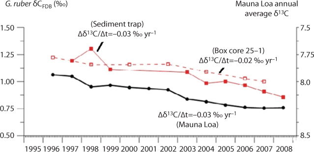
Figure 10.41 (b) Comparison of atmospheric CO2 and d13C to Cariaco Basin sediment trap and sediment core d13C. All three data sets indicate the same rate of d13C depletion (determined by linear regression), indicating that trap and core samples faithfully represent atmospheric trends (From Black et al., 2011).
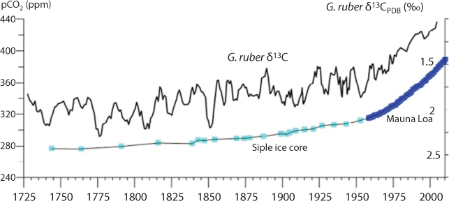
Figure 10.42 Planktonic foraminifera d13C over the last three centuries compared to Siple ice core and Mauna Loa pCO2.
Gravel et al. (2017) point out that in addition to the perturbation from fossil fuel emissions, atmospheric ∆14C was also subject to a large, abrupt perturbation in the 1950 s and 1960 s when a large amount of 14C was produced during atmospheric nuclear weapons testing. The introduction of this “bomb 14C” nearly doubled the amount of 14C in the Northern Hemisphere troposphere, where most of the tests took place. Most testing stopped after 1962 due to the Partial Test Ban Treaty, after which tropospheric ∆14C decreased quasi-exponentially as bomb 14C mixed through the atmosphere and into carbon reservoirs in the ocean and terrestrial biosphere that exchange with the atmosphere on annual to decadal timescales (Levin and Hesshaimer, 2000). Records of atmospheric ∆14C and δ13C have been extended into the past using measurements of tree rings and of CO2 in air from ice sheets. These records clearly show decreases in ∆14C and δ13C due to increased emissions of fossil-derived carbon following the Industrial Revolution and carbon from land use change. Ice cores, and tree ring and other proxy records, additionally reveal decadal to millennial variations associated with climate and carbon cycle variability, and, for 14C, changes in solar activity and the geomagnetic field (Damon et al., 1978).
Figure 10.43 shows for ∆14C in CO2 throughout the industrial age until modern era. The only increase in ∆14C relates to nuclear testing. As reported by Black et al. (2017), after 1955, ∆14C increased rapidly as a result of nuclear weapons testing, reaching a maximum of 836 ‰ in the Northern Hemisphere and 637 ‰ in the Southern Hemisphere, where the values 836 ‰ and 637 ‰ are the maxima in the forcing data. The ∆14C was even higher in the stratosphere and some Northern Hemisphere sites. After 1963– 1964, tropospheric ∆14C decreased quasi-exponentially as the nuclear test 14C mixed with oceanic and biospheric carbon reservoirs while growing fossil fuel emissions continued to dilute atmospheric 14CO2. Differences between the Northern and Southern Hemisphere reduced rapidly and were close to zero for the 1980s–1990s. The Northern Hemisphere deficit in ∆14C has been linked to a growing dominance of fossil fuel emissions in the Northern Hemisphere as air–sea exchange with 14C-depleted ocean water in C-depleted ocean water in the Southern Hemisphere weakened with decreasing atmospheric ∆14C (Graven et al., 2012).
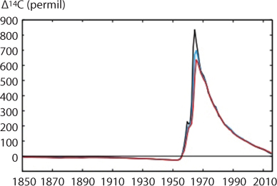
Figure 10.43 Historical atmospheric forcing datasets for D14C in CO2 (From Graven et al., 2017).
Figure 10.44 shows historical data for δ13C in atmospheric CO2 from ice core and firn records and from flask measurements to produce the historical atmospheric forcing dataset (Graven et al., 2017). There has been consistent decline in δ13C values with two distinct slopes. The fires slope that arises from 1850 remains constant until 1950, at which point the slope more than doubles. During the same time, there has been a consistent increase in oil production as North Sea and Alaska joined in the global oil production Figure 10.45.

Figure 10.44 Historical atmospheric forcing datasets for δ13C in CO2 (From Graven et al., 2017).
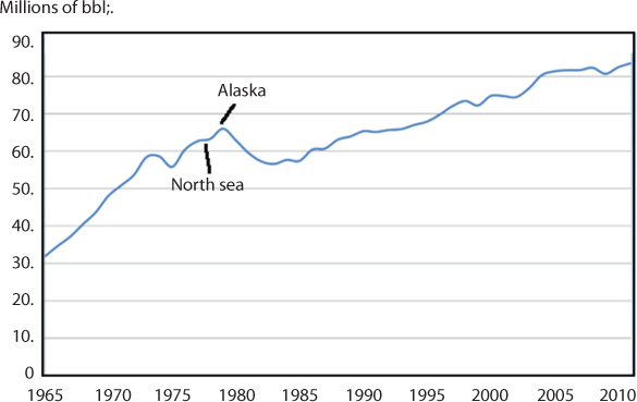
Figure 10.45 Global oil production during 1965-2010 (from Rapier, 2012).
10.7 The Role of Water in Global Warming
In overall functioning of the earth, water plays the most pivotal role. Water is ubiquitous and is plays a role at every stage of the carbon cycle, the important function being photosynthesis. Water is also the most potent solvent as well. In living cells, water is an ideal solvent as it is polar, meaning it can dissolve a variety of polar substances such as monosaccharides, amino acids, fatty acids, and vitamins and minerals, which can diffuse into the cells to help them survive by providing them with the metabolites to produce ATP for energy, allowing them to perform their particular functions. Minerals, in their natural form, are essential to metabolic activities. However, non-organic (as discussed in previous chapters) minerals (as well as vitamins) would disrupt normal functioning of all metabolic activities. In that sense, the composition of water is extremely important. Note that the composition should include so-called intangible components that are not detectible through conventional analytical tools. Ironically, at present, the most recent decadal increase in radiative forcing is attributable to CO2 (56%), CH4 (11%), N2O (6%) and CFCs(24%). Whereas, stratospheric H2O is estimated to have contributed only 4% (Shine et al., 1990).
Another vital function of water is in thermal properties. It is a terrific heat sink and it is resistant to changes in temperature due to strong hydrogen bonding between water molecules. For organic functioning, it means any effect of ambient temperature is sealed off by each cells or an organism. Thermal properties of water can be affected by the presence of metal particles that are not naturally occurring. This alteration can lead to snow ball effects, triggering chain of undesirable events.
Recently, Islam (2014) argued that water is the first material that resided on earth (and the universe). It means everything is ‘water-wet’. As a result, water can move along with great adhesion and cohesion properties. Water is highly cohesive. In fact, it is the highest of the non-metallic liquids. The positive and negative charges of the hydrogen and oxygen atoms that make up water molecules makes them attracted to each other. In a water molecule, the two hydrogen atoms align themselves along one side of the oxygen atom, with the result being that the oxygen side has a slight negative charge and the side with the hydrogen atoms has a slight positive charge. Thus when the positive side on one water molecule comes near the negative side of another water molecule, they attract each other and form a bond. This “bipolar” nature of water molecules gives water its cohesive nature. This property is also affected by the presence of artificial matter. The adhesive properties of water explain its capillary actions. Attraction to charged or polar surfaces allows water to flow in opposition of gravitational forces (capillary action). This capillary action is necessary to allow water to be transported up plant stems via a transpiration stream. Once again, metals play an important role in organic as well as non-organic systems, most notably in vascular systems. Studies over the past 40 years have revealed that the vascular system is much more than an organism’s “plumbing.” Rather than being a static series of pipes and tubes, the vascular system is extremely dynamic and plays a critical role, the functioning of which involves complex interactions among various vital parts, as discussed in many toxicology studies (Prozialeck et al., 2008). The exact behaviour is little known. Even less known is the extent of organic and non-organic chemicals affect organic functionalities.
Water viscosity is one of the most mysterious properties. Apparently, it is a Newtonian fluid with high resistance to temperature change. However, more recent studies indicate that water viscosity is very complex and far from being Newtonian (see Islam, 2014 for details). It also is affected by heavy metals, particularly in microscale. Reported sources of heavy metals in the environment include geogenic, industrial, agricultural, pharmaceutical, domestic effluents, and atmospheric sources (Tchounwou et al., 2012). Living organisms require varying amounts of heavy metals. Although, all metals are toxic at higher concentrations, non-organic metals are toxic at all concentrations (Long et al., 2002). In presence of non-organic form of heavy metals, a rigid viscosity barrier is created at nanolevel, leading to disruption of vital organic functions. The beneficial functions of heavy metals had been recognized in ancient medicinal practices that sought out herbs, rich in certain heavy metals (Singh et al., 2011). Natural phenomena such as weathering and volcanic eruptions have also been reported to significantly contribute to heavy metal pollution but the role of these naturally occurring heavy metals has not been studied, mainly because New Science cannot distinguish between these metals and artificially processed metals.
Non-organic heavy metals disrupt metabolic functions in two ways (Singh et al., 2011):
- They accumulate and thereby disrupt function in vital organic bodies.
- They displace the vital nutritional minerals from their original place, thereby, hindering their biological function.
In Point two above, it should be noted that anytime non-organic metal replaces organic metal components (within a nutrient body), it is far more damaging than an nonorganic molecule replacing another non-organic molecule.
Figure 10.46 Shows various mechanisms that are involved in transition metal accumulation by plants.They are (Yang et al., 2002):
- – Phytoaccumulation,
- – Phytoextraction,
- – phytovolatilization,
- – phytodegradation, and
- – phytostabilization.
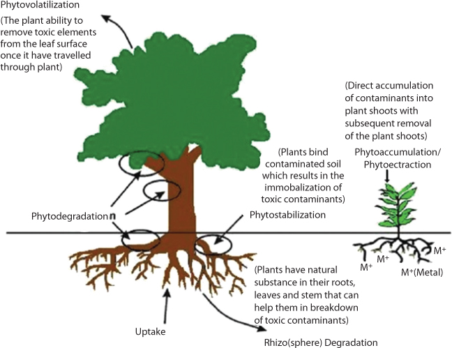
Figure 10.46 Transition mechanism in plants for metal accumulation (From Singh et al., 2011).
All these mechanisms will produce metabolic products that will be contaminated and will continue to act as ‘cancer’ for rest of their pathways. This is the source of that is referred earlier as Σaccumulation, which leads to Rejects at various stages of Calvin cycle.
10.7.1 Water as the Driver of Climate Change
The flow of water in different forms has a great role in climate change. Water is the main vehicle of natural transport phenomenon. A natural transport phenomenon is a flow of complex physical processes. The flow process consists of production, the storage and transport of fluids, electricity, heat, and momentum (Figure 10.47). The most essential material components of these processes are water and air, which are also the indicators of natural climate. Oceans, rivers, and lakes form both the source and the sink of major water transport systems. Because water is the most abundant matter on earth, any impact on the overall mass balance of water is certain to impact the global climate. The interaction between water and air in order to sustain life on this planet is a testimony to the harmony of nature. Water is the most potent solvent and also has very high heat storage capacity. Any movement of water through the surface and the Earth’s crust can act as a vehicle for energy distribution. However, the only source of energy is the sun and sunlight, the most essential ingredient for sustaining life on earth. The overall process in nature is inherently sustainable, yet truly dynamic. There isn’t one phenomenon that can be characterized as cyclic. Only recently, scientists have discovered that water has memory. Each phenomenon in nature occurs due to a driving force, such as pressure for fluid flow, electrical potential for the flow of electricity, thermal gradient for heat, and chemical potential for a chemical reaction. Natural transport phenomena cannot be explained by simple mechanistic views of physical processes described by a function of one variable.
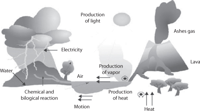
Figure 10.47 Natural transport phenomenon (Modified from Islam et al., 2010).
A simple flow model of natural transport phenomenon is presented in Figure 10.48. This model shows that nature has numerous interconnected processes, such as the production of heat, vapor, electricity and light, the storage of heat and fluid, and the flow of heat and fluids. All these processes continue for infinite time and are inherently sustainable. Any technologies that are based on natural principles are sustainable (Khan and Islam 2006). Water plays a crucial role in the natural climatic system. Water is the most essential as well as the most abundant ingredient of life. Just as water covers 70% of the earth’s surface, water constitutes 70% of the human body. Even though the value and sanctity of water has been well known for thousands of years in eastern cultures, scientists in the west are only now beginning to examine the concept that water has memory, and that numerous intangibles (most notably the pathway and intention behind human intervention) are important factors in defining the value of water (Islam, 2014).
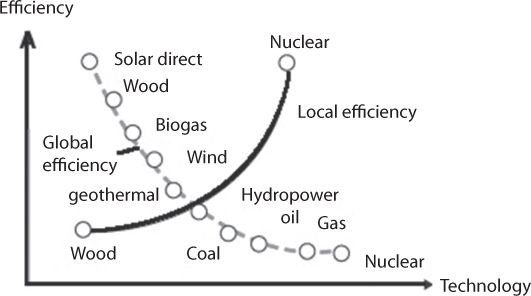
Figure 10.48 Global and local efficiency of different energy sources.
However, at the industrial/commercial level, preposterous treatment practices include the following: the addition of chlorine to “purify;” the use of toxic chemicals (soap) to get rid of dirt (the most potent natural cleaning agent) (Islam et al., 2015); the use of glycol (very toxic) for freezing or drying (getting rid of water) a product; the use of chemical CO2 to render water into a dehydrating agent (opposite to what is promoted as “refreshing”), then again to demineralize it by adding extra oxygen and ozone to “vitalize” it. The list seems to continue forever. Similar to what happens to food products (the degradation of the following chemical technology chain: Honey → Sugar → Saccharine → Aspartame), the chemical treatment technique promoted as water purification has taken a turn, spiraling downward (Khan and Islam, 2016). Chlorine treatment of water is common in the west and is synonymous with civilization. Similarly, transportation through copper pipes, distribution through stainless steel (enforced with heavy metal), storage in synthetic plastic containers and metal tanks, and mixing of ground water with surface water (collected from “purified” sewage water) are common practices in “developed” countries. More recent “innovations,” such as Ozone, UV, and even H2O2, are proving to be worse than any other technology. Overall, water remains the most abundant resource, yet “water war” is considered to be the most certain destiny of the 21st century. What Robert Curl (a Novel Laureate in Chemistry) termed as a “technological disaster,” modern technology development schemes seem to have targeted as the most abundant resource.
Water vapor is considered to be one of the major greenhouse gases in the atmosphere. The greenhouse gas effect is thought to be one of the major mechanisms by which the radiative factors of the atmosphere influence the global climate. Moreover, the radiative regime of the radiative characteristics of the atmosphere is largely determined by optically active components, such as CO2 and other gases, water vapor, and aerosols (Kondratyev and Cracknell 1998). As most of the incoming solar radiation passes through atmosphere and is absorbed by the Earth’s surface, the direct heating of the surface water and the evaporation of moisture results in heat transfer from the Earth’s surface to the atmosphere. The transport of heat by the atmosphere leads to the transient weather system. The latent heat, released due to the condensation of water vapors, and the clouds play an important role in reflecting incoming short-wave solar radiation and absorbing and emitting long wave radiation. Aerosols, such as volcanic dust and the particulates of fossil fuel combustion, are important factors in determining the behavior of the climate system. Kondratyev and Cracknell (1998) reported that the conventional method of calculating global warming potential only accounts for CO2, ignoring the contribution of water vapor and other gases in global warming. Their calculation scheme took into account the other components that affect the absorption of radiation, including CO2, water vapor, N2, O2, CH4, NOx, CO, SO2, nitric acid, ethylene, acetylene, ethane, formaldehyde, chlorofl uorocarbons, ammonia, and aerosol formation of different chemical composition and various sizes. However, this calculation fails to explain the effects of pure water vapor and the water vapor that is contaminated with chemical contaminants. The impact of water vapor on climate change depends on the quality of the water evaporated, its interaction with the atmospheric particulates of different chemical composition, and the size of the aerosols. There are at least 70,000 synthetic chemicals being used regularly throughout the world (Icenhower 2006). It has further been estimated that more than 1,000 chemicals are introduced every year. Billions of tons of fossil fuels are consumed each year to produce these chemicals that are the major sources of water and air contamination. The majority of these chemicals are very toxic and radioactive, and the particulates are continuously released into the atmosphere. The chemicals also reach water bodies by leakage, transportation loss, and as by-products of pesticides, herbicides, and water disinfectants. The industrial wastes, which are contaminated with these chemicals, also reach water bodies and contaminate the entire water system. The particulates of these chemicals and aerosols, when mixed with water vapor, may increase the absorption characteristics in the atmosphere, thereby increasing the possibility of trapping more heat. However, pure water vapor is one of the most essential components of the natural climate system and has no impacts on global warming. Moreover, most of the pure water vapors end up transforming into rain near the Earth’s surface and have no effect on the absorption and reflection. The water vapor in the warmer parts of the earth could rise to higher altitudes since they are more buoyant. As the temperature decreases in higher altitude, the water vapor gets colder, and it will hold less water vapor, reducing the possibility of increasing global warming. Because water is considered to have memory (Tschulakow et al. 2005), the assumption of water vapor’s impact on global warming cannot be explained without the knowledge of memory. The impact depends on the pathway water vapor travels before and after the formation of vapor from water. Gilbert and Zhang (2003) reported that nanoparticles change the crystal structure when they are wet. The structure change that takes place in the nanoparticles of water vapor and aerosols in the atmosphere has a profound impact on climate change. This relation has been explained based on the memory characteristics of water and analysis of its pathway. It is reported that water crystals are entirely sensitive to the external environment and take different shape based on the input (Emoto 2004). Moreover, the history of water memory can be traced by analysis of its pathway. The memory of water might have a significant role to play in technological development (Hossain and Islam, 2008). Recent attempts have been made towards understanding the role of history on the fundamental properties of water. These models take into account the intangible properties of water, and this line of investigation can address the global warming phenomenon. The memory of water not only has impacts on energy and ecosystems but also plays a key role in the global climate scenario.
10.8 Characterization of Energy Sources
10.8.1 Environmental and Ecological Impact
Each process has an environmental impact, either positive or negative. The positive impacts are expected to keep an ecological balance. Most of the processes that are established to-date are disrupting ecological balances and produce enormous negative effects on all living beings. For instance, the use of Freon in cooling systems, disrupts the ozone layer, allowing vulnerable rays from the sun to penetrate the earth and to living beings. Burning of “chemically purified” fossil fuels also pollutes the environment by releasing harmful chemicals. Energy extraction from nuclear technology leaves harmful spent residues. The environmental impact of different processes has been discussed by Islam et al. (2010).
10.8.2 Quality of Energy
The quality of energy is an important phenomenon. However, when it comes to energy, the talk about quality is largely absent. In the same spirit as “chemicals are chemical” that launched the mass production of various food and drugs, irrespective of their origins and pathways, energy is promoted as just “energy”, based on the spurious basis that “photons are the units of all energy”. Only recently, has it come to light that artificial chemicals act exactly opposite to how natural products do (Chhetri and Islam, 2007). Miralai et al. (2007) recently discussed the reason behind such behavior. According to them, chemicals with exactly the same molecular formulae derived from different sources cannot have the same effect unless the same pathways are followed. With this theory, it is possible to explain why organic products are beneficial while chemical products are not. Similarly, heating from different sources of energy cannot have the same impact. Heating of homes by wood is a natural burning process, which was practiced since ancient times and did not cause any negative effects to humans. More recently, Khan and Islam (2007) extended the “chemicals are chemicals” analogy to “energy is energy”. They argued that energy sources cannot be characterized by heating value alone. Using a similar argument, Chhetri and Islam (2008) established a scientific criterion for characterizing energy sources and demonstrated that conventional evaluation would lead to misleading conclusions if the scientific value (rather than simply “heating value”) of an energy source was ignored. On the other hand, Knipe and Jennings (2007), indicated a number of vulnerable health effects to human beings due to chronic exposure of electrical heating. The radiation due to the electro-magnetic rays might cause interference with the human’s radiation frequency which can cause acute long-term damage to humans. Energy with natural frequency is the most desirable. Alternate current is not natural and that’s why there will be some vulnerable effects of this frequency to the environment and humans (Chhetri, 2007). That is why it can be inferred that heating by natural sources is better than heating by electricity. Microwave heating is also questionable. Vikram et al. (2005) reported that the nutrient of orange juice degraded highest by microwave oven heating as compared to other heating methods. It has been reported that microwave cooking destroys more than 97% of the flavonoids in broccoli and causes a 55% chlorogenic acid loss in potatoes. A 65% quercetin content loss is also reported in tomatoes (Vallejo et al., 2003). There are several other compounds formed during electric and electromagnetic cooking which are considered to be carcinogenic, based on their pathway analysis.
10.8.3 Evaluation of Process
From the above discussion, it can be noted that considering only the energy efficiency based on input and output of a process does not identify the most efficient process. All of the factors should be considered and carefully analyzed to claim a process efficient in the long-term. The evaluation process of an efficient process should consider both the efficiency and the quality of a process. Considering the material characterization developed by Khan and Islam (2012), the selection of a process can be evaluated using the following equations:
(10.28)
Where Ereal is the true efficiency of a process when long term factors are considered, E is the efficiency at present time (t =“right now”), E0 is the baseline efficiency, and δ(s) is the sustainability index, introduced by Khan (2007), such that”
δ(s) = 1, if the technology is sustainable; and
δ(s) = –1, if the technology is not sustainable.
(10.29)
Where Qreal is the quality of the process. L (t) is the alteration of quality of a process as a function of time.
When both Ereal and Qreal have positive values, this make the process acceptable. However, the most efficient process will be the one which has highest product value (Ereal × Qreal). After evaluation of efficient processes, economic evaluation can be made to find the most economical one. Today’s economic evaluation of any contemporary process, based on tangible benefits provides the decision to establish the process for commercial applications. However, decision making for any process needs to evaluate a number of criteria, as discussed earlier. Moreover, the economics of intangibles should be analyzed thoroughly to decide on the best solutions. Time span may be considered to be the most important intangible in this economic consideration. Considering the long-term, tangible and intangible effects, natural processes are considered to be the best solutions. However, to arrive at any given end-product, any number of natural processes may be available. Selection of the best natural one depends on what objectives have the greatest priority at each stage and what objectives can be accomplished within a given span of time. If the time span is considered important, it is required to find out the natural process which will either have a low pay back period or a high rate of return., is this right?, However, irrespective of time span, the best natural process to select would be that which will base itself on the process which renders the best quality output, with no immediate impacts and no long-term ones.
10.8.4 Final Characterization
Various energy sources are classified based on a set of newly developed criteria. Energy is conventionally classified, valued, or measured based on the absolute output of a system. The absolute value represents the steady state of an energy source. However, modern science recognizes that such a state does not exist and every form of energy is at a state of flux. This section characterizes various energy sources based on their pathways. Each form of energy has a set of characteristic features. Anytime these features are violated through human intervention, the quality of the energy form declines. This analysis enables one to assign a greater quality index to a form of energy that is closest to its natural state. Consequently, the heat coming from wood burning and the heat coming from electrical power will have different impacts on the quality of heat. Just as all chemicals are not the same, different forms of heat coming from different energy sources are not the same. The energy sources are based on the global efficiency of each technology, the environmental impact of the technology, and the overall value of energy systems (Chhetri and Islam, 2008). Energy sources are classified based on the age of the fuel source in nature as it is transformed from one form to another (Chhetri et al. 2006). Various energy sources are also classified according to their global efficiency. Conventionally, energy efficiency is defined for a component or service as the amount of energy required in the production of that component or service, e.g., the amount of cement that can be produced with one billion Btu of energy. Energy efficiency is improved when a given level of service is provided with reduced amounts of energy inputs or when services or products are increased for a given amount of energy input. However, the global efficiency of a system is calculated based on the energy input, product output, the possibility of multiple uses of energy in the system, the use of the system’s by-products, and its impacts to the environment. The global efficiency calculation considers the source of the fuel, the pathways the energy system travels, conversion systems, impacts on human health and the environment, and by-products of the energy system. Islam et al. (2010) calculated the global efficiency of various energy systems. They showed that global efficiencies of higher quality energy sources are higher than those of lower quality energy sources. With their ranking, a solar energy source (when applied directly) is the most efficient (because the source is free and
has no negative environmental impacts), while nuclear energy is the least efficient, among many other forms of energy studied. They demonstrated that previous findings failed to discover this logical ranking because the focus had been on local efficiency. For instance, nuclear energy is generally considered to be highly efficient, which is a true observation if one’s analysis is limited to one component of the overall process. If global efficiency is considered, the fuel enrichment alone involves numerous centrifugation stages. This enrichment alone will render the global efficiency very low.
Carbon dioxide is characterized based on normally-ignored criteria such as its origin, the pathway it travels, the isotope number and age of the fuel source from which it was emitted. Fossil fuel exploration, production, processing, and consumption are major sources of carbon dioxide emissions. Here, various energy sources are characterized based on their efficiency, environmental impact, and quality of energy based on the new criteria. Different energy sources follow different paths from origin to end-use and contribute emissions differently. A detailed analysis has been carried out on potential precursors to global warming. The focus is on supplying a scientific basis as well as practical solutions after identifying the roots of the problem. Similarly, this chapter presents an evaluation of existing models on global warming, based on the scenario of various protocols and agreements, including the Paris Agreement. Shortcomings in the conventional models have been identified based on this evaluation. The sustainability of conventional global warming models has been argued. Here, these models are deconstructed and new models are developed based on new sustainability criteria. Conventional energy production and processing use various toxic chemicals and catalysts that are harmful to the environment.