Chapter 7: Running a Tiny CIFAR-10 Model on a Virtual Platform with the Zephyr OS

Prototyping a TinyML application directly on a physical device is really fun because we can instantly see our ideas at work in something that looks and feels like the real thing. However, before any application comes to life, we need to ensure that the models work as expected and, possibly, among different devices. Testing and debugging applications directly on microcontroller boards often requires a lot of development time. The main reason for this is the necessity to upload a program into a device for every change in code. However, virtual platforms can come in handy to make testing more straightforward and faster.

In this chapter, we will build an image classification application with TensorFlow Lite for Microcontrollers (TFLu) for an emulated Arm Cortex-M3 microcontroller. We will start by installing the Zephyr OS, the primary framework used in this chapter to accomplish our task. Next, we will design a tiny quantized CIFAR-10 model with TensorFlow (TF). This model will be capable of running on a microcontroller with only 256 KB of program memory and 64 KB of RAM. In the end, we will deploy an image classification application on an emulated Arm Cortex-M3 microcontroller through Quick Emulator (QEMU).

The aim of this chapter is to learn how to build and run a TFLu-based application with the Zephyr OS on a virtual platform and provide practical advice on the design of an image classification model for memory-constrained microcontrollers.

In this chapter, we're going to implement the following recipes:

• Getting started with the Zephyr OS
• Designing and training a tiny CIFAR-10 model
• Evaluating the accuracy of the TFLite model
• Converting a NumPy image to a C-byte array
• Preparing the skeleton of the TFLu project
• Building and running the TFLu application on QEMU

Technical requirements

To complete all the practical recipes of this chapter, we will need the following:

• A laptop/PC with either Ubuntu 18.04+ or later on x86_64

The source code and additional material are available in the Chapter07 file (https://github.com/PacktPublishing/TinyML-Cookbook/tree/main/Chapter07).

Getting started with the Zephyr OS

In this recipe, we will install the Zephyr project, the framework used in this chapter to build and run the TFLu application on the emulated Arm Cortex-M3 microcontroller. At the end of this recipe, we will check whether everything works as expected by running a sample application on the virtual platform considered for our project.

Getting ready

To get started with this first recipe, we need to know what the Zephyr project is about.

Zephyr (https://zephyrproject.org/) is an open source Apache 2.0 project that provides a small-footprint Real-Time Operating System (RTOS) for various hardware platforms based on multiple architectures, including Arm Cortex-M, Intel x86, ARC, Nios II, and RISC-V. The RTOS has been designed for memory-constrained devices with security in mind.

Zephyr does not provide just an RTOS, though. It also offers a Software Development Kit (SDK) with a collection of ready-to-use examples and tools to build Zephyr-based applications for various supported devices, including virtual platforms through QEMU.

QEMU (https://www.qemu.org/) is an open source machine emulator that allows us to test programs without using real hardware. The Zephyr SDK supports two QEMU Arm Cortex-M-based microcontrollers, which are as follows:

• The BBC micro:bit (https://microbit.org/) with the Arm Cortex-M0
• Texas Instruments' LM3S6965 (https://www.ti.com/product/LM3S6965) with the Arm Cortex-M3

From the preceding two QEMU platforms, we will use the LM3S6965. Our choice fell to the Texas Instruments board because it has a bigger RAM capacity than the BBC micro:bit. In fact, although the devices have the same program memory size (256 KB), LM3S6965 has 64 KB of RAM. Unfortunately, the BBC micro:bit has only 16 KB of RAM, not enough for running a CIFAR-10 model.

How to do it…

The Zephyr installation consists of the following steps:

1. Installing Zephyr prerequisites
2. Getting Zephyr source code and related Python dependencies
3. Installing the Zephyr SDK

   Important Note

   The installation guide reported in this section refers to Zephyr 2.7.0 and the Zephyr SDK 0.13.1.

Before getting started, we recommend you have the Python Virtual Environment (virtualenv) tool installed to create an isolated Python environment. If you haven't installed it yet, open your terminal and use the following pip command:

$ pip install virtualenv

To launch the Python virtual environment, create a new directory (for example, zephyr):

$ mkdir zephyr && cd zephyr

Then, create a virtual environment inside the directory just created:

$ python -m venv env

The preceding command creates the env directory with all the executables and Python packages required for the virtual environment.

To use the virtual environment, you just need to activate it with the following command:

$ source env/bin/activate

If the virtual environment is activated, the shell will be prefixed with (env):

(env)$

Tip

You can deactivate the Python virtual environment at any time by typing deactivate in the shell.

The following steps will help you prepare the Zephyr environment and run a simple application on the virtual Arm Cortex-M3-based microcontroller:

1. Follow the instructions reported in the Zephyr Getting Started Guide (https://docs.zephyrproject.org/2.7.0/getting_started/index.html) until the Install a Toolchain section. All Zephyr modules will be available in the ~/zephyrproject directory.
2. Navigate into the Zephyr source code directory and enter the samples/synchronization folder:

   $ cd ~/zephyrproject/zephyr/samples/synchronization

Zephyr provides ready-to-use applications in the samples/ folder to demonstrate the usage of RTOS features. Since our goal is to run an application on a virtual platform, we consider the synchronization sample because it does not require interfacing with external components (for example, LEDs).

3. Build the pre-built synchronization sample for qemu_cortex_m3:

   $ west build -b qemu_cortex_m3 .

The sample test is compiled with the west command (https://docs.zephyrproject.org/latest/guides/west/index.html). West is a tool developed by Zephyr to manage multiple repositories conveniently with a few command lines. However, West is more than a repository manager. In fact, the tool can also plug additional functionalities through extensions. Zephyr exploits this pluggable mechanism to offer the commands to compile, flash, and debug applications (https://docs.zephyrproject.org/latest/guides/west/build-flash-debug.html).

The west command used to compile the application has the following syntax:

$ west build -b <BOARD> <EXAMPLE-TO-BUILD>

Let's break down the preceding command:

• <BOARD>: This is the name of the target platform. In our case, it is the QEMU Arm Cortex-M3 platform (qemu_cortex_m3).
• <EXAMPLE-TO-BUILD>: This is the path to the sample test to compile.

Once we have built the application, we can run it on the target device.

4. Run the synchronization example on the LM3S6965 virtual platform:

   $ west build -t run

To run the application, we just need to use the west build command, followed by the build system target (-t) as a command-line argument. Since we had specified the target platform when we built the application, we can simply pass the run option to upload and run the program on the device.

If Zephyr is installed correctly, the synchronization sample will run on the virtual Arm Cortex-M3 platform and print the following output:

threadA: Hello World from arm!

threadB: Hello World from arm!

threadA: Hello World from arm!

threadB: Hello World from arm!

You can now close QEMU by pressing Ctrl + A.

Designing and training a tiny CIFAR-10 model

The tight memory constraint on LM3S6965 forces us to design a model with extremely low memory utilization. In fact, the target microcontroller has four times less memory capacity than Arduino Nano.

Despite this challenging constraint, in this recipe, we will be leveraging the following tiny model for the CIFAR-10 image classification, capable of running on LM3S6965:

Figure 7.1 – A model tailored for CIFAR-10 dataset image classification

The preceding network will be designed with TF and the Keras API.

The following Colab file (in the Designing and training a tiny CIFAR-10 model section) contains the code referred to in this recipe:

• prepare_model.ipynb

(https://github.com/PacktPublishing/TinyML-Cookbook/blob/main/Chapter07/ColabNotebooks/prepare_model.ipynb).

Getting ready

The network tailored in this recipe takes inspiration from the success of the MobileNet V1 on the ImageNet dataset classification. Our model aims to classify the 10 classes of the CIFAR-10 dataset: airplane, automobile, bird, cat, deer, dog, frog, horse, ship, and truck.

The CIFAR-10 dataset is available at https://www.cs.toronto.edu/~kriz/cifar.html and consists of 60,000 RGB images with 32 x 32 resolution.

To understand why the proposed model can run successfully on LM3S6965, we want to outline the architectural design choices that make this network suitable for our target device.

As shown in Figure 7.1, the model has a convolution base, which acts as a feature extractor, and a classification head, which takes the learned features to perform the classification.

Early layers have large spatial dimensions and low Output Feature Maps (OFMs) to learn simple features (for example, simple lines). Deeper layers, instead, have small spatial dimensions and a high OFMs to learn complex features (for example, shapes).

The model uses pooling layers to halve the spatial dimensionality of the tensors and reduce the risk of overfitting when increasing the OFM. Generally, we want several activation maps for deep layers to combine as many complex features as possible. Therefore, the idea is to get smaller spatial dimensions to afford more OFMs.

In the following subsection, we will explain the design choice in using Depthwise Separable Convolution (DWSC) layers instead of the standard convolution 2D.

Replacing convolution 2D with DWSC

DWSC is the layer that made MobileNet V1 a success on the ImageNet dataset and the heart of our proposed convolution-based architecture. This operator took the lead in MobileNet V1 to produce an accurate model that can also run on a device with limited memory and computational resources.

As seen in Chapter 5, Indoor Scene Classification with TensorFlow Lite for Microcontrollers and the Arduino Nano, and shown in the following figure, DWSC is a depthwise convolution followed by a convolution layer with a 1 x 1 kernel size (that is, pointwise convolution):

Figure 7.2 – The DWSC

To demonstrate the efficiency of this operator, consider the first DWSC layer in the network presented in Figure 7.1. As shown in the following diagram, the input tensor has a 32 x 32 x 16 dimension while the output tensor has a 32 x 32 x 24 dimension:

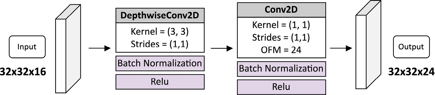
Figure 7.3 – The first DWSC in the CIFAR-10 model

If we replace the DWSC with a regular convolution 2D with a 3 x 3 filter size, we will need 3,480 trainable parameters, of which 3,456 are weights (3 x 3 x 16 x 24), and 24 are biases. The DWSC, instead, just needs 560 trainable parameters, distributed as follows:

• 144 weights and 16 biases for the depthwise convolution layer with a 3 x 3 filter size
• 384 weights and 24 biases for the pointwise convolution

Therefore, in this particular case, the DWSC layer yields roughly six times fewer trainable parameters than a regular convolution 2D layer.

The model size reduction is not the only benefit this layer offers. The other advantage in using the DWSC is given by the reduction of the arithmetic operations. In fact, although both layers are made of several Multiply-Accumulate (MAC) operations, the DWSC needs considerably fewer MAC operations than convolution 2D.

This aspect is demonstrated by the following two formulas for the calculation of the total MAC operations for convolution 2D and the DWSC:

The formula is broken down as follows:

• : The total MAC operations for convolution 2D
• : The total MAC operations for the DWSC
• : The filter size
• : The width and height of the output tensor
• : The number of input and output feature maps

The calculation of the total MAC for the DWSC has two parts. The first part calculates the MAC operations for depthwise convolution, assuming that the input and output tensors have the same feature maps. The second part calculates the MAC operations for the pointwise convolution.

If we use the preceding two formulas for the case reported in Figure 7.3, we will discover that convolution 2D needs 3,583,944 operations while DWSC needs only 540,672 operations. Therefore, there is a computational complexity reduction of over six times with DWSC.

Hence, the efficiency of the DWSC layer is double since it decreases the trainable parameters and arithmetic operations involved.

Now that we know the benefits of this layer, let's discover how to design a model that can run on our target device.

Keeping the model memory requirement under control

Our goal is to produce a model that can fit in 256 KB of program memory and run with 64 KB of RAM. The program memory usage can be obtained directly from the .tflite model generated. Alternatively, you can check the Total params value returned by the Keras summary() method (https://keras.io/api/models/model/#summary-method) to have an indication of how big the model will be. Total params represents the number of trainable parameters, and it is affected mainly by the OFM and layers. In our case, the convolution base has five trainable layers with a maximum of 192 activation maps. This choice will make our model utilize just 30% of the total program memory.

The estimation of the RAM utilization is a bit more complicated and depends upon the model architecture. All the non-constant variables, such as the network input, output, and intermediate tensors, stay in RAM. However, although the network may need several tensors, TFLu has a memory manager capable of efficiently providing portions of memory at runtime. For a sequential model such as ours, where each layer has one input and one output tensor, a ballpark figure for the RAM utilization is given by the sum of the following:

• The memory required for the model input and output tensors
• The two largest intermediate tensors

In our network, the first DWSC produces the largest intermediate tensor with 24,576 elements (32 x 32 x 24), as shown in the following figure:

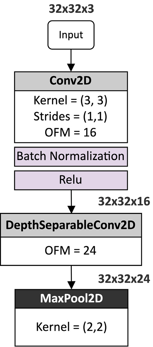
Figure 7.4 – The first DWSC produces the biggest intermediate tensor

As you can see from the preceding diagram, the first DWSC produces a tensor with 24 OFMs, which we found as a good compromise between accuracy and RAM utilization. However, you may consider reducing this further to make the model even smaller and more performant.

How to do it…

Create a new Colab project and follow these steps to design and train a quantized CIFAR-10 model with TFLite:

1. Download the CIFAR-10 dataset:

   (train_imgs, train_lbls), (test_imgs, test_lbls) = datasets.cifar10.load_data()

2. Normalize the pixel values between 0 and 1:

   train_imgs = train_imgs / 255.0

   test_imgs = test_imgs / 255.0

This step ensures that all data is on the same scale.

3. Define a Python function to implement the DWSC:

   def separable_conv(i, ch):

       x = layers.DepthwiseConv2D((3,3), padding="same")(i)

       x = layers.BatchNormalization()(x)

       x = layers.Activation("relu")(x)

       x = layers.Conv2D(ch, (1,1), padding="same")(x)

       x = layers.BatchNormalization()(x)

       return layers.Activation("relu")(x)

The separable_conv() function accepts the following input arguments:

• i: Input to feed to the depthwise convolution 2D
• ch: The number of OFMs to produce

The batch normalization layer standardizes the input to a layer and makes the model training faster and more stable.

4. Design the convolution base, as described in Figure 7.1:

   input = layers.Input((32,32,3))

   x = layers.Conv2D(16, (3, 3), padding='same')(input)

   x = layers.BatchNormalization()(x)

   x = layers.Activation("relu")(x)

   x = separable_conv(0, x, 24)

   x = layers.MaxPooling2D((2, 2))(x)

   x = separable_conv(0, x, 48)

   x = layers.MaxPooling2D((2, 2))(x)

   x = separable_conv(0, x, 96)

   x = separable_conv(0, x, 192)

   x = layers.MaxPooling2D((2, 2))(x)

We use pooling layers to reduce the spatial dimensionality of the feature maps through the network. Although we can use DWSC with non-unit strides to accomplish a similar sub-sampling task, we preferred pooling layers to keep the number of trainable parameters low.

5. Design the classification head:

   x = layers.Flatten()(x)

   x = layers.Dropout(0.2)(x)

   x = layers.Dense(10)(x)

6. Generate the model and print its summary:

   model = Model(input, x)

   model.summary()

As shown in the following screenshot, the model summary returns roughly 60,000 parameters:

Figure 7.5 – A CIFAR-10 model summary (trainable parameters)

In the case of 8-bit quantization, 60,000 floating-point parameters correspond to 60,000 8-bit integer values. Therefore, the weights contribute to the model size with 60 KB, well away from the 256 KB maximum target. However, we should not consider this number as the model size, since what we deploy on a microcontroller is the TFLite file, which also contains the network architecture and the quantization parameters.

A ballpark figure for the RAM utilization can be estimated from the tensor size of each intermediate tensor in the network. This information can be extrapolated from the output of model.summary(). As anticipated in the previous Getting ready section, the intermediate tensors of the first DWSC layer have the largest number of elements. The following screenshot is taken from the output of model.summary() and reports the tensor shapes for these two tensors:

Figure 7.6 – A CIFAR-10 model summary (the first DWSC)

As you can see from the DWSC area marked in the preceding screenshot, the tensors with the largest number of elements are as follows:

• The output of act0_dwsc2: (None, 32, 32, 16)
• The output of conv0_dwsc2: (None, 32, 32, 24)

Therefore, the expected memory utilization for the intermediate tensor should be in the order of 41 KB. To this number, we should add the memory for the input and output nodes to get a more precise ballpark figure of the RAM usage. The input and output tensors need 3,082 bytes, of which 3,072 bytes are for the input and 10 bytes are for the output. In total, we expect to use 44 KB of RAM during the model inference, which is less than the 64 KB target.

Note

In Figure 7.6, there are three layers with the (None, 32, 32, 16) output shape: conv0_dwsc2, bn1_dwsc2, and act1_dwsc2. However, only the pointwise convolution layer (conv0_dwsc2) counts for memory utilization of the intermediate tensors because batch normalization (bn1_dwsc2) and activation (act1_dwsc2) will be fused into the convolution (conv0_dwsc2) by the TFLite converter.

7. Compile and train the model with 10 epochs:

   model.compile(optimizer='adam', loss = tf.keras.losses.SparseCategoricalCrossentropy(from_logits=True), metrics=['accuracy'])

   model.fit(train_imgs, train_lbls, epochs=10, validation_data=(test_imgs, test_lbls))

After 10 epochs, the model should obtain an accuracy of 73% on the validation dataset.

8. Save the TF model as SavedModel:

   model.save("cifar10")

Our CIFAR-10 model is now ready for being quantized with the TFLite converter.

Evaluating the accuracy of the TFLite model

The tiny model just trained can classify the 10 classes of CIFAR-10 with an accuracy of 73%. However, what is the model's accuracy of the quantized variant generated by the TFLite converter?

In this recipe, we will quantize the model with the TFLite converter and show how to perform this accuracy evaluation on the test dataset with the TFLite Python interpreter. After the accuracy evaluation, we will convert the TFLite model to a C-byte array.

The following Colab file (the Evaluating the accuracy of the quantized model section) contains the code referred to in this recipe:

• prepare_model.ipynb:

https://github.com/PacktPublishing/TinyML-Cookbook/blob/main/Chapter07/ColabNotebooks/prepare_model.ipynb.

Getting ready

In this section, we will explain why the accuracy of the TFLite model may differ from the trained one.

As we know, the trained model needs to be converted to a more compact and lightweight representation before being deployed on a resource-constrained device such as a microcontroller.

Quantization is the essential part of this step to make the model small and improve the inference performance. However, post-training quantization may change the model accuracy because of the arithmetic operations at a lower precision. Therefore, it is crucial to check whether the accuracy of the generated .tflite model is within an acceptable range before deploying it into the target device.

Unfortunately, TFLite does not provide a Python tool for the model accuracy evaluation. Hence, we will use the TFLite Python interpreter to accomplish this task. The interpreter will allow us to feed the input data to the network and read the classification result. The accuracy will be reported as the fraction of samples correctly classified from the test dataset.

How to do it…

Follow these steps to evaluate the accuracy of the quantized CIFAR-10 model on the test dataset:

1. Select a few hundred samples from the train dataset to calibrate the quantization:

   cifar_ds = tf.data.Dataset.from_tensor_slices(train_images).batch(1)

   def representative_data_gen():

       for i_value in cifar_ds.take(100):

            i_value_f32 = tf.dtypes.cast(i_value, tf.float32)

            yield [i_value_f32]

The TFLite converter uses the representative dataset to estimate the quantization parameters.

2. Initialize the TFLite converter to perform the 8-bit quantization:

   tflite_conv = tf.lite.TFLiteConverter.from_saved_model("cifar10")

   tflite_conv.representative_dataset = tf.lite.RepresentativeDataset(representative_data_gen)

   tflite_conv.optimizations = [tf.lite.Optimize.DEFAULT]

   tflite_conv.target_spec.supported_ops = [tf.lite.OpsSet.TFLITE_BUILTINS_INT8]

   tflite_conv.inference_input_type = tf.int8

   tflite_conv.inference_output_type = tf.int8

For quantizing the TF model to 8-bit, we import the SavedModel directory (cifar10) into the TFLite converter and enforce full integer quantization.

3. Convert the model to the TFLite file format and save it as .tflite:

   tfl_model = tfl_conv.convert()

   open("cifar10.tflite", "wb").write(tfl_model)

4. Evaluate the TFLite model size:

   print(len(tfl_model))

The expected model size is 81,304 bytes. As you can see, the model can fit in 256 KB of program memory.

5. Evaluate the accuracy of the quantized model using the test dataset. To do so, start the TFLite interpreter and allocate the tensors:

   tfl_inter = tf.lite.Interpreter(model_content=tfl_model)

   tfl_inter.allocate_tensors()

Get the quantization parameters of the input and output nodes:

i_details = tfl_inter.get_input_details()[0]

o_details = tfl_inter.get_output_details()[0]

i_quant = i_details["quantization_parameters"]

i_scale      = i_quant['scales'][0]

i_zero_point = i_quant['zero_points'][0]

o_scale      = o_quant['scales'][0]

o_zero_point = o_quant['zero_points'][0]

Initialize a variable to zero (num_correct_samples) to keep track of the correct classifications:

num_correct_samples = 0

num_total_samples   = len(list(test_imgs))

Iterate over the test samples:

for i_value, o_value in zip(test_imgs, test_lbls):

    input_data = i_value.reshape((1, 32, 32, 3))

    i_value_f32 = tf.dtypes.cast(input_data, tf.float32)

Quantize each test sample:

    i_value_f32 = i_value_f32 / i_scale + i_zero_point

    i_value_s8 = tf.cast(i_value_f32, dtype=tf.int8)

Initialize the input node with the quantized sample and start the inference:

    tfl_conv.set_tensor(i_details["index"], i_value_s8)

    tfl_conv.invoke()

Read the classification result and dequantize the output to a floating point:

    o_pred = tfl_conv.get_tensor(o_details["index"])[0]

    o_pred_f32 = (o_pred - o_zero_point) * o_scale

Compare the classification result with the expected output class:

    if np.argmax(o_pred_f32) == o_value:

         num_correct_samples += 1

6. Print the accuracy of the quantized TFLite model:

   print("Accuracy:", num_correct_samples/num_total_samples)

After a few minutes, the accuracy result will be printed in the output log. The expected accuracy should still be around 73%.

7. Convert the TFLite model to a C-byte array with xxd:

   !apt-get update && apt-get -qq install xxd

   !xxd -i cifar10.tflite > model.h

You can download the model.h and cifar10.tflite files from Colab's left pane.

Converting a NumPy image to a C-byte array

Our application will be running on a virtual platform with no access to a camera module. Therefore, we need to supply a valid test input image into our application to check whether the model works as expected.

In this recipe, we will get an image from the test dataset that must return a correct classification for the ship class. The sample will then be converted to an int8_t C array and saved as an input.h file.

The following Colab file (refer to the Converting a NumPy image to a C-byte array section) contains the code referred to in this recipe:

• prepare_model.ipynb:

https://github.com/PacktPublishing/TinyML-Cookbook/blob/main/Chapter07/ColabNotebooks/prepare_model.ipynb

Getting ready

To get ready for this recipe, we just need to know how to prepare the C file containing the input test image. The structure of this file is quite simple and reported in the following figure:

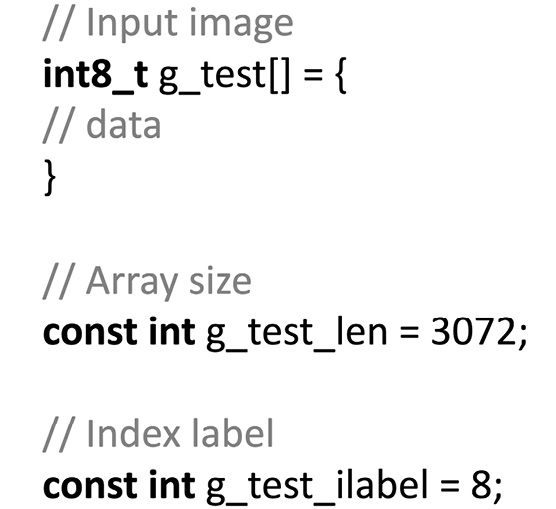
Figure 7.7 – The C header file structure for the input test image

As you can observe from the file structure, we only need an array and two variables to describe our input test sample, which are as follows:

• g_test: An int8_t array containing a ship image with the normalized and quantized pixel values. The pixels stored in the array (// data) should be comma-separated integer values.
• g_test_len: An integer variable for the array size. Since the input model is an RGB image with a 32 x 32 resolution, we expect an array with 3,072 int8_t elements.
• g_test_ilabel: An integer variable for the class index of the input test image. Since we have a ship image, the expected class index is eight.

The input image will be obtained from the test dataset. Therefore, we will need to implement a function in Python to convert an image stored in NumPy format to a C array.

How to do it…

Follow the these steps to generate a C header file containing a ship image from the test dataset:

1. Write a function to convert a 1D NumPy array of np.int8 values into a single string of comma-separated integer values:

   def array_to_str(data):

       NUM_COLS = 12

       val_string = ''

       for i, val in enumerate(data):

            val_string += str(val)

            if (i + 1) < len(data):

                 val_string += ','

            if (i + 1) % NUM_COLS == 0:

                 val_string += ' '

       return val_string

In the preceding code, the NUM_COLS variable limits the number of values on a single row. In our case, NUM_COLS is set to 12 so that we can add a newline character after every 12 values.

2. Write a function to generate a C header file containing the input test image stored in an int8_t array. To do so, you can have a template string with the following fields:
   • The size of the array (size)
   • The values to put in the array (data)
   • The index of the class assigned to the input image (ilabel)

   def gen_h_file(size, data, ilabel):

       str_out = f'int8_t g_test[] = '

       str_out += " { "

       str_out += f'{data}'

       str_out += '}; '

       str_out += f"const int g_test_len = {size}; "

       str_out += f"const int g_test_ilabel = {ilabel}; "

       return str_out

As you can see from the preceding code, the function expects {data} to be a single string of comma-separated integer values.

3. Create a pandas DataFrame from the CIFAR-10 test dataset:

   imgs = list(zip(test_imgs, test_lbls))

   cols = [Image, 'Label']

   df = pd.DataFrame(imgs, columns = cols)

4. Get only ship images from the pandas DataFrame:

   cond = df['Label'] == 8

   ship_samples = df[cond]

In the preceding code, 8 is the index for the ship class.

5. Iterate over the ship images and run the inference:

   c_code = ""

   for index, row in ship_samples.iterrows():

       i_value = np.asarray(row['Image'].tolist())

       o_value = np.asarray(row['Label'].tolist())

       o_pred_f32 = classify(i_value, o_value)

6. Check whether the classification returns a ship. If so, convert the input image into a C-byte array and exit the loop:

       if np.argmax(o_pred_f32) == o_value:

            i_value_f32 = i_value / i_scale + i_zero_point

            i_value_s8  = i_value_f32.astype(dtype=np.uint8)

            i_value_s8  = i_value_s8.ravel()

            # Generate a string from NumPy array

            val_string = array_to_str(i_value_s8)

            # Generate the C header file

            c_code = gen_h_file(         i_value_s8.size, val_string, "8")

            break

7. Save the generated code in the input.h file:

   with open("input.h", 'w') as file:

       file.write(c_code)

You can download the input.h file containing the input test image from Colab's left pane.

Preparing the skeleton of the TFLu project

Only a few steps are separating us from the completion of this project. Now that we have the input test image, we can leave Colab's environment and focus on the application with the Zephyr OS.

In this recipe, we will prepare the skeleton of the TFLu project from the pre-built TFLu hello_world sample available in the Zephyr SDK.

The following C files contain the code referred to in this recipe:

• main.c, main_functions.cc, and main_functions.h:

https://github.com/PacktPublishing/TinyML-Cookbook/blob/main/Chapter07/ZephyrProject/Skeleton

Getting ready

This section aims to provide the basis for starting a new TFLu project with the Zephyr OS from scratch.

The easiest way to create a project is to copy and edit one of the pre-built samples for TFLu. The samples are available in the ~/zephyrproject/zephyr/samples/modules/tflite-micro folder. At the time of writing, there are two ready-to-use examples:

• hello_world: A sample showing the basics of TFLu to replicate a sine function: https://docs.zephyrproject.org/latest/samples/modules/tflite-micro/hello_world/README.html
• magic_wand: A sample showing how to implement a TFLu application to recognize gestures with accelerometer data: https://docs.zephyrproject.org/latest/samples/modules/tflite-micro/hello_world/README.html

In this recipe, we will base our application on the hello_world application, and the following screenshot shows what you should find in the sample directory:

Figure 7.8 – The contents of the hello_world sample folder

The hello_world folder contains three subfolders, but only src/ is of interest to us because it contains the source code for the application. However, not all the files in src/ are essential for our project. For example, assert.cc, constants.h, constants.c, model.cc, model.h, output_handler.cc, and output_handler.h are only required for the sine wave sample application. Therefore, the only C files needed for a new TFLu project are as follows:

• main.c: This file contains the standard C/C++ main() function, responsible for starting and terminating the program execution. The main() function consists of a setup() function called once and a loop() function executed 50 times. Therefore, the main function replicates more or less the behavior of an Arduino program.
• main_functions.h and main_functions.cc: These files contain the declaration and definition of the setup() and loop() functions.

In the end, the CMakeList.txt and prj.conf files in the hello_world directory are required for building the application. We will learn more about these files in the last recipe of this chapter.

How to do it…

Open the terminal and follow these steps to create a new TFLu project:

1. Navigate into the ~/zephyrproject/zephyr/samples/modules/tflite-micro/ directory and create a new folder named cifar10:

   $ cd ~/zephyrproject/zephyr/samples/modules/tflite-micro/

   $ mkdir cifar10

2. Copy the content of the hello_world directory to cifar10:

   $ cp -r hello_world/* cifar10

3. Navigate into the cifar10 directory and remove the following files from the src/ directory:

constants.h, constants.c, model.c, model.h, output_handler.cc, output_handler.h, and assert.cc

These files can be removed because they are only required for the sine wave sample application, as explained in the Getting ready section of this recipe.

4. Copy the model.h and input.h files generated in the previous two recipes into the cifar10/src folder.

Once you have copied the files, the cifar10/src folder should contain the following files:

Figure 7.9 – The contents of the hello_word/src folder

Before continuing, ensure you have the files listed in the previous screenshot.

Now, open your default C editor (for example, Vim) to make some code changes in the main.c and main_functions.cc files.

5. Open the main.c file and replace for (int i = 0; i < NUM_LOOPS; i++) with while(true). The code in the main.c file should become the following:

   int main(int argc, char *argv[]) {

       setup();

       while(true) {

            loop();

       }

       return 0;

   }

This preceding code replicates exactly the behavior of an Arduino sketch, where setup() is called once and loop() is repeated indefinitely.

6. Open main_functions.cc and remove the following:
   • constants.h and output_handler.h from the list of header files.
   • The inference_count variable and all its usages. This variable will not be required in our application.
   • The code within the loop() function.

Next, replace g_model with the name of the array in model.h. The g_model variable is used when calling tflite::GetModel().

Now that we have the project structure ready, we can finally implement our application.

Building and running the TFLu application on QEMU

The skeleton of our Zephyr project is ready, so we just need to finalize our application to classify our input test image.

In this recipe, we will see how to build the TFLu application and run the program on the emulated Arm Cortex-M3-based microcontroller.

The following C files contain the code referred to in this recipe:

• main.c, main_functions.cc, and main_functions.h:

https://github.com/PacktPublishing/TinyML-Cookbook/blob/main/Chapter07/ZephyrProject/CIFAR10

Getting ready

Most of the ingredients required for developing this recipe are related to TFLu and have already been discussed in earlier chapters, such as Chapter 3, Building a Weather Station with TensorFlow Lite for Microcontrollers, or Chapter 5, Indoor Scene Classification with TensorFlow Lite for Microcontrollers and the Arduino Nano. However, there is one small detail of TFLu that has a big impact on the program memory usage that we haven't discussed yet.

In this section, we will talk about the tflite::MicroMutableOpResolver interface.

As we know from our previous projects, the TFLu interpreter is responsible for preparing the computation for a given model. One of the things that the interpreter needs to know is the function pointer for each operator to run. So far, we have provided this information with tflite::AllOpsResolver. However, tflite::AllOpsResolver is not recommended because of the heavy program memory usage. For example, this interface will prevent building our application because of the low program memory capacity on the target device. Therefore, TFLu offers tflite::MicroMutableOpResolver, an alternative and more efficient interface to load only the operators required by the model. To know which different operators the model needs, you can visualize the TFLite model (.tflite) file with the Netron web application (https://netron.app/).

How to do it…

Let's start this recipe by visualizing the architecture of our TFLite CIFAR-10 model file (cifar10.tflite) with Netron.

The following screenshot shows a slice of our model visualized with this tool:

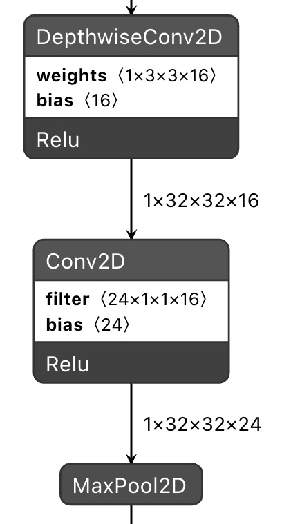
Figure 7.10 – A visualization of a slice of the CIFAR-10 model in Netron (courtesy of netron.app)

Inspecting the model with Netron, we can see that the model only uses five operators: Conv2D, DepthwiseConv2D, MaxPool2D, Reshape, and FullyConnected. This information will be used to initialize tflite::MicroMutableOpResolver.

Now, open your default C editor and open the main_functions.cc file.

Follow these steps to build the TFLu application:

1. Use the #include directives to add the header file of the input test image (input.h):

   #include "input.h"

2. Increase the arena size (tensor_arena_size) to 52,000:

   constexpr int tensor_arena_size = 52000;

   Note

   The original variable name for the tensor arena is kTensorArenaSize. To keep consistency with the lower_case naming convention used in the book, we have renamed this variable to tensor_arena_size.

The TFLu tensor arena is the portion of memory allocated by the user to accommodate the network input, output, intermediate tensors, and other data structures required by TFLu. The arena size should be a multiple of 16 to have a 16-byte data alignment.

As we have seen from the design of the CIFAR-10 model, the expected RAM usage for the model inference is in the order of 44 KB. Therefore, 52,000 bytes is okay for our case because it is greater than 44 KB, a multiple of 16, and less than 64 KB, the maximum RAM capacity.

3. Replace uint8_t tensor_arena[tensor_arena_size] with uint8_t *tensor_arena = nullptr:

   uint8_t *tensor_arena = nullptr;

The tensor arena is too big for being placed in the stack. Therefore, we should dynamically allocate this memory in the setup() function.

4. Declare a global tflite::MicroMutableOpResolver object to load only the operations needed for running the CIFAR-10 model:

   tflite::MicroMutableOpResolver<5> resolver;

This object is created by providing the maximum number of different operations that the model requires as a template argument.

5. Declare two global variables for the output quantization parameters:

   float o_scale = 0.0f;

   int32_t o_zero_point = 0;

6. In the setup() function, remove the instantiation of the tflite::AllOpsResolver object. Next, load the operators used by the model into the tflite::MicroMutableOpResolver object (resolver) before the initialization of the TFLu interpreter:

   resolver.AddConv2D();

   resolver.AddDepthwiseConv2D();

   resolver.AddMaxPool2D();

   resolver.AddReshape();

   resolver.AddFullyConnected();

   static tflite::MicroInterpreter static_interpreter(model, resolver, tensor_arena, tensor_arena_size, error_reporter);

   interpreter = &static_interpreter;

7. In the setup() function, get the output quantization parameters from the output tensor:

   const auto* o_quantization = reinterpret_cast<TfLiteAffineQuantization*>(output->quantization.params);

   o_scale      = o_quantization->scale->data[0];

   o_zero_point = o_quantization->zero_point->data[0];

8. In the loop() function, initialize the input tensor with the content of the input test image:

     for(int i = 0; i < g_test_len; i++) {

          input->data.int8[i] = g_test[i];

     }

Next, run the inference:

  TfLiteStatus invoke_status = interpreter->Invoke();

9. After the model inference, return the output class with the highest score:

     size_t ix_max = 0;

     float  pb_max = 0;

     for (size_t ix = 0; ix < 10; ix++) {

       int8_t out_val = output->data.int8[ix];

       float  pb = ((float)out_val - o_zero_point) * o_scale;

       if(pb > pb_max) {

            ix_max = ix;

            pb_max = pb;

       }

   }

The preceding code iterates over the quantized output values and returns the class (ix_max) with the highest score.

10. In the end, check whether the classification result (ix_max) is equal to the label index assigned to the input test image (g_test_label):

    if(ix_max == g_test_ilabel) {

If so, print CORRECT classification! and return the classification result:

    static const char *label[] = {"airplane", "automobile", "bird", "cat", "deer", "dog", "frog", "horse", "ship", "truck"};

    printf("CORRECT classification! %s ", label[ix_max]);

    while(1);

}

Now, open the terminal, and use the following command to build the project for qemu_cortex_m3:

$ cd ~/zephyrproject/zephyr/samples/modules/tflite-micro/cifar10

$ west build -b qemu_cortex_m3 .

After a few seconds, the west tool should display the following output in the terminal, confirming that the program has been successfully compiled:

Figure 7.11 – The memory usage summary

From the summary generated by the west tool, you can see that our CIFAR-10-based application uses 52.57% of program memory (FLASH) and 6.92% of RAM (SRAM). However, we should not be misled by RAM usage. In fact, the summary does not consider the memory that we allocate dynamically. Therefore, to the 4,536 bytes statically allocated in RAM, we should add the 52,000 bytes of the tensor arena, which brings us to 88% of RAM utilization.

Now that the application is built, we can run it on the virtual platform with the following command:

$ west build -t run

The west tool will boot the virtual device and return the following output, confirming that the model correctly classified the image as a ship:

Figure 7.12 – The expected output after the model inference

As you can see from the preceding screenshot, the virtual device outputs the CORRECT classification message, confirming the successful execution of our tiny CIFAR-10 model!

Join us on Discord!

Do not miss out on the opportunity to take your reading experience beyond the pages. We have a dedicated channel on the Embedded System Professionals community over Discord for you to read the book with other users.

Join now to share your journey with the book, discuss queries with other users and the author, share advice with others wherever you can, and importantly build your projects in collaboration with so many other users who have already joined us on the book club.

See you on the other side!

https://discord.com/invite/UCJTV3A2Qp