Chapter 4: Voice Controlling LEDs with Edge Impulse

Keyword spotting (KWS) is a technology applied in a wide range of daily-life applications to enable an entirely hands-free experience with the device. The detection of the famous wake-up words OK Google, Alexa, Hey Siri, or Cortana represents a particular usage of this technology, where the smart assistant continuously listens for the magic phrase before starting to interact with the device.

Since KWS aims to identify utterances from real-time speech, it needs to be on-device, always-on, and running on a low-power system to be effective.

This chapter demonstrates the usage of KWS through Edge Impulse by building an application to voice control the light-emitting diode (LED)-emitting color (red, green, and blue (or RGB)) and the number of times to make it blink (one, two, and three times).

This TinyML application could find space in smart educational toys to learn both color and number vocabulary with peace of mind regarding privacy and security since it does not require internet connectivity.

This chapter will start focusing on the dataset preparation, showing how to acquire audio data with a mobile phone. Next, we will design a model based on Mel-frequency cepstral coefficients (MFCC), one of the most popular features for speech recognition. In these recipes, we will show how to extract MFCCs from audio samples, train the machine learning (ML) model, and optimize the performance with the EON Tuner. At the end of the chapter, we will concentrate on finalizing the KWS application on the Arduino Nano and the Raspberry Pi Pico.

This chapter is intended to show how to develop an end-to-end (E2E) KWS application with Edge Impulse and get familiar with audio data acquisition and analog-to-digital converter (ADC) peripherals.

In this chapter, we're going to implement the following recipes:

• Acquiring audio data with a smartphone
• Extracting MFCC features from audio samples
• Designing and training a neural network (NN) model
• Tuning model performance with EON Tuner
• Live classifications with a smartphone
• Live classifications with the Arduino Nano
• Continuous inferencing on the Arduino Nano
• Building the circuit with the Raspberry Pi Pico to voice control LEDs
• Audio sampling with ADC and timer interrupts on the Raspberry Pi Pico

Technical requirements

To complete all the practical recipes of this chapter, we will need the following:

• An Arduino Nano 33 BLE Sense board
• A Raspberry Pi Pico board
• Smartphone (Android phone or Apple iPhone)
• Micro Universal Serial Bus (USB) cable
• 1 x half-size solderless breadboard
• 1 x electret microphone amplifier - MAX9814 (Raspberry Pi Pico only)
• 11 x jumper wires (Raspberry Pi Pico only)
• 2 x 220 Ohm resistor (Raspberry Pi Pico only)
• 1 x 100 Ohm resistor (Raspberry Pi Pico only)
• 1 x red LED (Raspberry Pi Pico only)
• 1 x green LED (Raspberry Pi Pico only)
• 1 x blue LED (Raspberry Pi Pico only)
• 1 x push-button (Raspberry Pi Pico only)
• Laptop/PC with either Ubuntu 18.04+ or Windows 10 on x86-64

The source code and additional material are available in the Chapter04 folder of the GitHub repository (https://github.com/PacktPublishing/TinyML-Cookbook/tree/main/Chapter04).

Acquiring audio data with a smartphone

As for all ML problems, data acquisition is the first step to take, and Edge Impulse offers several ways to do this directly from the web browser.

In this recipe, we will learn how to acquire audio samples using a mobile phone.

Getting ready

Acquiring audio samples with a smartphone is the most straightforward data acquisition approach offered by Edge Impulse because it only requires a phone (Android phone or Apple iPhone) with internet connectivity.

However, how many samples do we need to train the model?

Collecting audio samples for KWS

The number of samples depends entirely on the nature of the problem—therefore, no appraoch fits all. For a situation such as this, 50 samples for each class could be sufficient to get a basic model. However, 100 or more are generally recommended to get better results. We want to give you complete freedom on this choice. However, remember to get an equal number of samples for each class to obtain a balanced dataset.

Whichever dataset size you choose, try including different variations in the instances of speech, such as accents, inflations, pitch, pronunciations, and tone. These variations will make the model capable of identifying words from different speakers. Typically, recording audio from persons of different ages and genders should cover all these cases.

Although there are six output classes to identify (red, green, blue, one, two, and three), we should consider an additional class for cases when anyone is speaking or there are unknown words in the speech.

How to do it…

Open the Edge Impulse Dashboard and give a name to your project (for example, voice_controlling_leds).

Note

In this recipe, N will be used to refer to the number of samples for each output class.

Follow the next steps to acquire audio data with the mobile phone's microphon:

1. Click on Let's collect some data from the Acquire data section.

Then, click on Show QR code on the Use your mobile phone option from the menu:

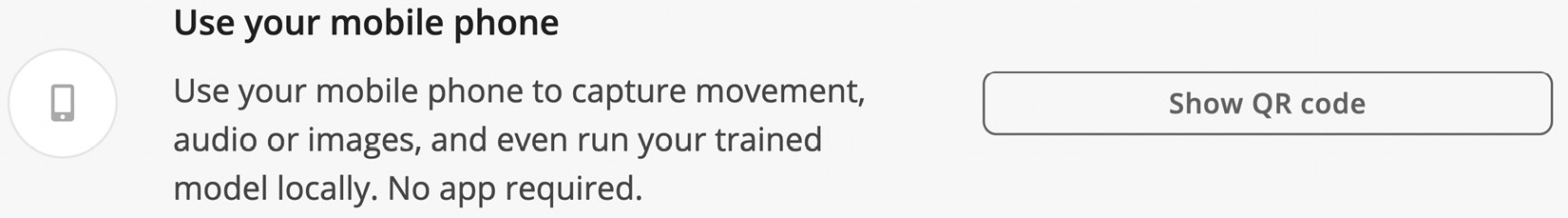
Figure 4.1 – Clicking on the Show QR code to pair the mobile phone with Edge Impulse

Scan the Quick Response (QR) code with your smartphone to pair the device with Edge Impulse. A pop-up window on your phone will confirm that the device is connected, as shown in the following screenshot:

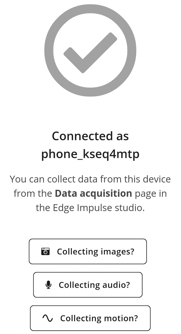
Figure 4.2 – Edge Impulse message on your phone

On your mobile phone, click on Collecting audio? and give permission to use the microphone.

Since it is not required to have a laptop and smartphone in the same network, we could collect audio samples anywhere. As we can guess, this approach is well suited to recording sounds from different environments since it only requires a phone with internet connectivity.

2. Record N (for example, 50) utterances for each class (red, green, blue, one, two, and three). Before clicking on Start recording, set Category to Training and enter one of the following labels in the Label field, depending on the spoken word:

Figure 4.3 – Labels for the output categories

Since the label encoding assigns an integer value based on alphabetical ordering to each output category, our proposed names (00_red, 01_green, 02_blue, 03_one, 04_two, and 05_three) will be helpful to know whether we have a color or a number from the label index easily. For example, if the label index is less than 3, we have a color.

We recommend repeating the same utterance several times in a single recording to avoid uploading too many files into Edge Impulse. For example, you could record audio of 20 seconds (s) where you repeat the same word 10 times with a 1-s pause in between.

The recordings will be available in the Data acquisition section. By clicking on the file, you can visualize the corresponding audio waveform:

Figure 4.4 – Audio waveform

The raw audio waveform is the signal recorded by the microphone and graphically describes the sound-pressure variation over time. The vertical axis reports the amplitude of this vibration, while the horizontal axis reports the time. The higher waveform amplitude implies louder audio as perceived by the human ear.

3. Split the recordings containing repetitions of the utterance in individual samples by clicking on near the filename and then clicking on Split sample, as shown in the following screenshot:

Figure 4.5 – Split sample option

Edge Impulse will automatically detect spoken words, as you can observe from the following screenshot:

Figure 4.6 – Audio waveform with repetitions of the same utterance

Set the segment length to 1000 milliseconds (ms) (1 s), and ensure all the samples are centered within the cutting window. Then, click on Split to get the individual samples.

4. Download the keyword dataset from Edge Impulse (https://cdn.edgeimpulse.com/datasets/keywords2.zip) and unzip the file. Import N random samples from the unknown dataset into the Edge Impulse project. Go to Data acquisition and click on the Upload existing data button from the Collect data menu:

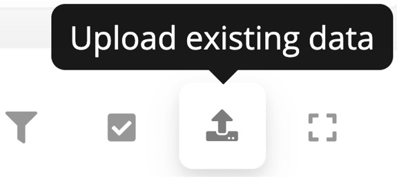
Figure 4.7 – Button to upload existing training data

On the UPLOAD DATA page, do the following:

• Set Upload category to Training.
• Write unknown in the Enter label field.

Click on Begin upload to import the files into the dataset.

5. Split the samples between training and test datasets by clicking on the Perform train / test split button in the Danger zone area of the Dashboard:

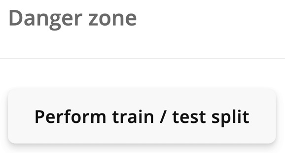
Figure 4.8 – Danger zone in Edge Impulse

Edge Impulse will ask you twice if you are sure about this action because the data shuffling is irreversible.

You should now have 80% of the samples assigned to the training/validation set and 20% to the test one.

Extracting MFCC features from audio samples

When building an ML application with Edge Impulse, the impulse is responsible for all of the data processing, such as feature extraction and model inference.

In this recipe, we will see how to design an impulse to extract MFCC features from the audio samples.

Getting ready

Let's start this recipe by discussing what an impulse is and examining the MFCC features used for our KWS application.

In Edge Impulse, an impulse is responsible for data processing and consists of two computational blocks, mainly the following:

• Processing block: This is the preliminary step in any ML application, and it aims to prepare the data for the ML algorithm.
• Learning block: This is the block that implements the ML solution, which aims to learn patterns from the data provided by the processing block.

The processing block determines the ML effectiveness since the raw input data is often not suitable for feeding the model directly. For example, the input signal could be noisy or have irrelevant and redundant information for training the model, just to name a few scenarios.

Therefore, Edge Impulse offers several pre-built processing functions, including the possibility to have custom ones.

In our case, we will use the MFCC feature extraction processing block, and the following subsections will help us learn more about this.

Analyzing audio in the frequency domain

In contrast to vision applications where convolutional NNs (CNNs) can make feature extraction part of the learning process, typical speech recognition models do not perform well with raw audio data. Therefore, feature extraction is required and needs to be part of the processing block.

We know from physics that sound is the vibration of air molecules that propagates as a wave. For example, if we played a pure single tone, the microphone would record a sine signal:

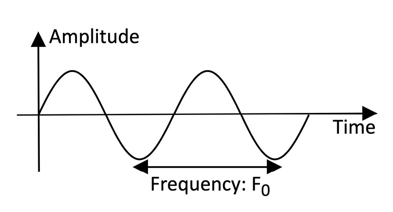
Figure 4.9 – Sine waveform

Although the sounds in nature are far from pure, every sound can be expressed as the sum of sine waves at different frequencies and amplitudes.

Since a frequency and amplitude characterize sine waves, we commonly represent the components in the frequency domain through the power spectrum:

Figure 4.10 – Representation of a signal in the frequency domain

The power spectrum reports the frequency on the horizontal axis and the power (S) associated with each component on the vertical axis.

The Discrete Fourier Transform (DFT) is the required mathematical tool to decompose a digital audio waveform in all its constituent sine waves, commonly called components.

Now that we are familiar with the frequency representation of an audio signal, let's see what we can generate as an input feature for a CNN.

Generating a mel spectrogram

A spectrogram can be considered an audio signal's image representation because it visually shows the power spectrum over time.

A spectrogram is obtained by splitting the audio waveform into smaller segments and applying the DFT on each one, as shown in the following screenshot:

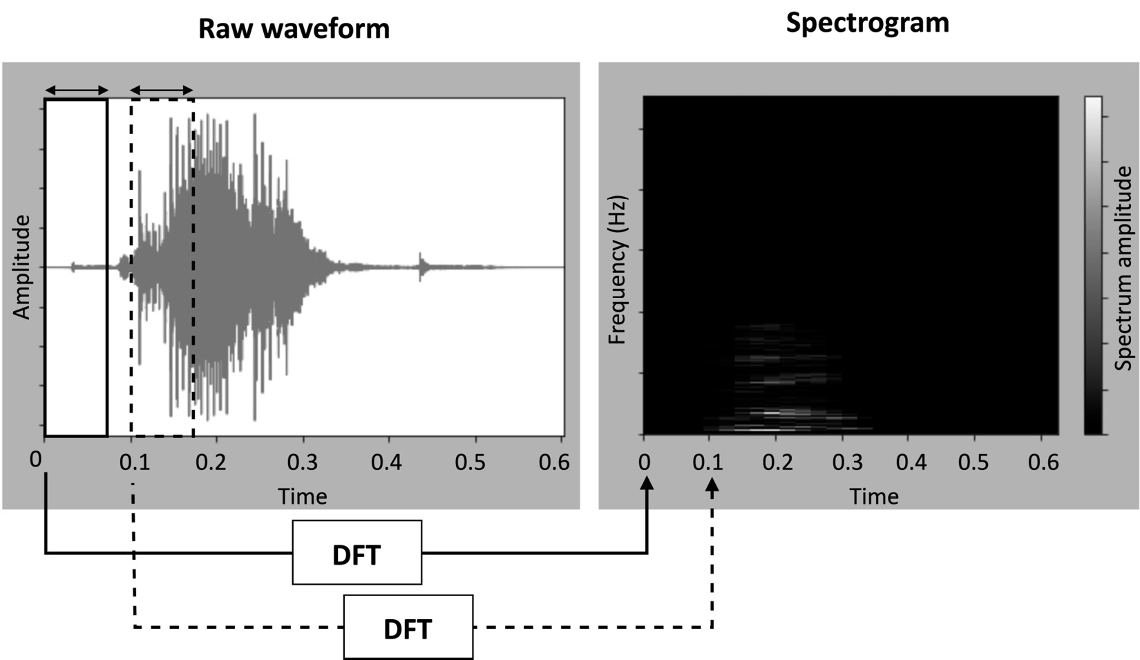
Figure 4.11 – Audio waveform and spectrogram of the red utterance

In the spectrogram, each vertical slice represents the power spectrum associated with each segment—in particular:

• The width reports the time.
• The height reports the frequency.
• The color reports the power spectrum amplitude, so a brighter color implies a higher amplitude.

However, a spectrogram obtained in this way would be ineffective for voice speech recognition because the relevant features are not emphasized. In fact, as we can observe from the preceding screenshot, the spectrogram is dark in almost all regions.

Therefore, the spectrogram is adjusted considering that humans perceive frequencies and loudness on a logarithmic scale rather than linearly. These adjustments are as follows:

• Scaling the frequency (hertz, or Hz) to Mel with the Mel scale filter bank: The Mel scale remaps the frequencies to make them distinguishable and perceived equidistantly. For example, if we played pure tones from 100 Hz to 200 Hz with a 1 Hz step, we could distinctly perceive all 100 frequencies. However, if we conducted the same experiment at higher frequencies (for example, between 7500 Hz and 7600 Hz), we could barely hear all tones. Therefore, not all frequencies are equally important for our ears.

The Mel scale is commonly computed using triangular filters overlapped (filter bank) in the frequency domain.

• Scaling the amplitudes using the decibel (dB) scale: The human brain does not perceive amplitude linearly but logarithmically, as with frequencies. Therefore, we scale the amplitudes logarithmically to make them visible in the spectrogram.

The spectrogram obtained by applying the preceding transformations is a mel spectrogram or Mel-frequency energy (MFE). The MFE of the red word using 40 triangular filters is reported in the following screenshot, where we can now clearly notice the intensity of the frequency components:

Figure 4.12 – Spectrogram and Mel spectrogram of the red utterance

Although the mel spectrogram works well with audio recognition models, there is also something more efficient for human speech recognition regarding the number of input features—the MFCC.

Extracting the MFCC

MFCC aims to extract fewer and highly unrelated coefficients from the mel spectrogram.

The Mel filter bank uses overlapped filters, which makes the components highly correlated. If we deal with human speech, we can decorrelate them by applying the Discrete Cosine Transform (DCT).

The DCT provides a compressed version of the filter bank. From the DCT output, we can keep the first 2-13 coefficients (cepstral coefficients) and discard the rest because they do not bring additional information for human speech recognition. Hence, the resulting spectrogram has fewer frequencies than the mel spectrogram (13 versus 40).

How to do it…

We start designing our first impulse by clicking on the Create impulse option from the left-hand side menu, as shown in the following screenshot:

Figure 4.13 – Create impulse option

In the Create impulse section, ensure the time-series data has the Window size field set to 1000 ms and the Window increase field to 500 ms.

Window increase is a parameter specifically for continuous KWS applications, where there is a continuous audio stream and we do not know when the utterance starts. In this scenario, we should split the audio stream into windows (or segments) of equal length and execute the ML inference on each one. Window size is the temporal length of the window, while Window increase is the temporal distance between two consecutive segments, as shown in the following diagram:

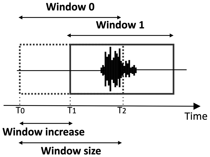
Figure 4.14 – Window size versus Window increase

The Window size value depends on the training sample length (1 s) and may affect the accuracy results. On the contrary, the Window increase value does not impact the training results but affects the chances of getting a correct start of the utterance. In fact, a smaller Window increase value implies a higher probability. However, the suitable Window increase value will depend on the model latency.

The following steps show how to design a processing block for extracting MFCC features from recorded audio samples:

1. Click on the Add a processing block button and add Audio (MFCC).
2. Click on the Add a learning block button and add Classification (Keras).

The Output features block should report the seven output classes to recognize (00_red, 01_green, 02_blue, 03_one, 04_two, 05_three, and unknown), as shown in the following screenshot:

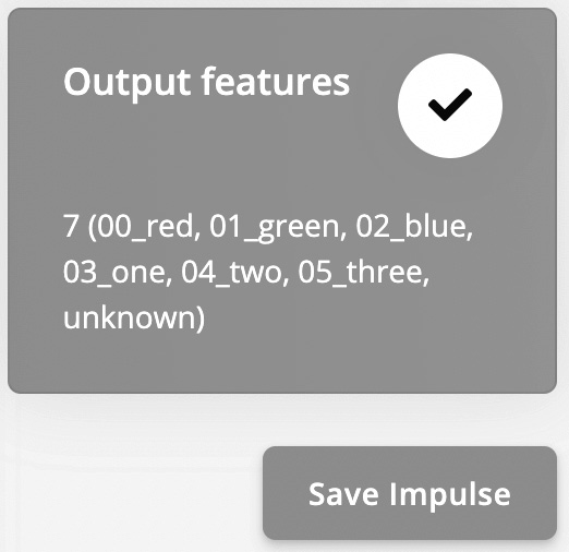
Figure 4.15 – Output features

Save the impulse by clicking on the Save Impulse button.  

3. Click on MFCC from the Impulse design category. In the new window, we can play on the parameters affecting the extraction of MFCC features, such as the number of cepstral coefficients, the number of triangular filters applied for the Mel scale, and so on. All the MFCC parameters are kept at their default values.

At the bottom of the page, there are also two parameters for the pre-emphasis stage. The pre-emphasis stage is performed before generating a spectrogram to reduce the effect of noise by increasing energy at the highest frequencies. If the Coefficient value is 0, there is no pre-emphasis on the input signal. The pre-emphasis parameters are kept at their default values.

4. Extract the MFCC features from each training sample by clicking on the Generate features button:

Figure 4.16 – Generate features button

Edge Impulse will return Job completed in the console output at the end of this process.

MFCC features are now extracted from all the recorded audio samples.

There's more…

Once MFCCs have been generated, we can use the Feature explorer tool to examine the generated training dataset in a three-dimensional (3D) scatter plot, as shown in the following screenshot:

Figure 4.17 – Feature explorer showing the seven output classes

From the Feature explorer chart, we should infer whether the input features are suitable for our problem. If so, the output classes (except the unknown output category) should be well separated.

Under the Feature explorer area, we find the On-device performance section related to MFCC:

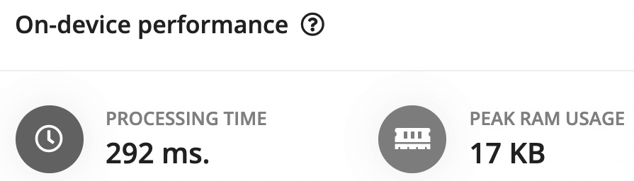
Figure 4.18 – MFCC performance on the Arduino Nano 33 BLE Sense board

PROCESSING TIME (latency) and PEAK RAM USAGE (data memory) are estimated considering the target device selected in Dashboard | Project info:

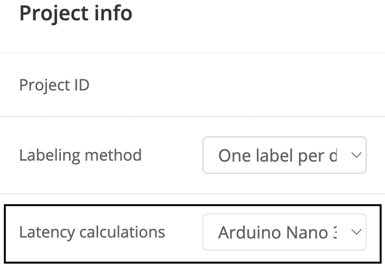
Figure 4.19 – Target device reported in Project info

From Project info, you can change the target device for performance estimation.

Unfortunately, Edge Impulse does not support the Raspberry Pi Pico, so the estimated performance will only be based on the Arduino Nano.

Designing and training a NN model

In this recipe, we will be leveraging the following NN architecture to recognize our words:

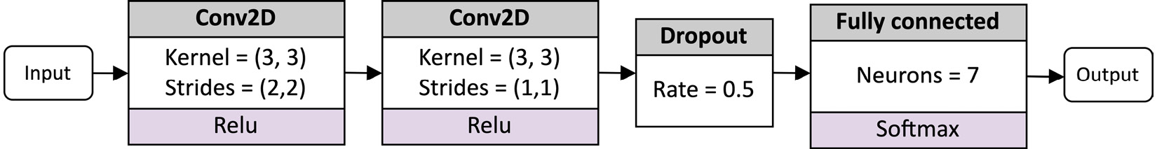
Figure 4.20 – NN architecture

The model has two two-dimensional (2D) convolution layers, one dropout layer, and one fully connected layer, followed by a softmax activation.

The network's input is the MFCC feature extracted from the 1-s audio sample.

Getting ready

To get ready for this recipe, we just need to know how to design and train a NN in Edge Impulse.

Depending on the learning block chosen, Edge Impulse exploits different underlying ML frameworks for training. For a classification learning block, the framework uses TensorFlow with Keras. The model design can be performed in two ways:

• Visual mode (simple mode): This is the quickest way and through the user interface (UI). Edge Impulse provides some basic NN building blocks and architecture presets, which are beneficial if you have just started experimenting with deep learning (DL).
• Keras code mode (expert mode): If we want more control over the network architecture, we can edit the Keras code directly from the web browser.

Once we have designed the model, we can launch the training from the same window.

How to do it…

Click on Neural Network (Keras) under Impulse design and follow the next steps to design and train the NN presented in Figure 4.20:

1. Select the 2D Convolutional architecture preset and remove the Dropout layer between the two convolution layers:

Figure 4.21 – Deleting the dropout layer between the two 2D convolution layers

2. Switch to Keras (expert) mode by clicking on . In the coding area, delete the MaxPooling2D layers:

Figure 4.22 – Deleting the two pooling layers from the Keras code

Set the strides of the first convolution layer to (2,2):

model.add(Conv2D(8, strides=(2,2), kernel_size=3, activation='relu', kernel_constraint=tf.keras.constraints.MaxNorm(1), padding='same'))

The pooling layer is a subsampling technique that reduces information propagated through the network and lowers the overfitting risk. However, this operator may increase latency and random-access memory (RAM) usage. In memory-constraint devices such as microcontrollers, memory is a precious resource, and we need to use it as efficiently as possible. Therefore, the idea is to adopt non-unit strides in convolution layers to reduce spatial dimensionality. This approach is typically more performant because we skip the pooling layer computation entirely, and we can have faster convolution layers, given fewer output elements to process.

3. Launch the training by clicking on the Start training button:

Figure 4.23 – Start training button

The output console will report the accuracy and loss on the training and validation datasets during training after each epoch.

At the end of the training, we can evaluate the model's performance (accuracy and loss), the confusion matrix, and the estimated on-device performance on the same page.

Important Note

If you achieve 100% accuracy, this is a sign that the model is likely overfitting the data. To avoid this issue, you can either add more data to your training set or reduce the learning rate.

If you are not happy with the model's accuracy, we recommend collecting more data and training the model again.

Tuning model performance with EON Tuner

Developing the most efficient ML pipeline for a given application is always challenging. One way to do this is through iterative experiments. For example, we can evaluate how some target metrics (latency, memory, and accuracy) change depending on the input feature generation and the model architecture. However, this process is time-consuming because there are several combinations, and each one needs to be tested and evaluated. Furthermore, this approach requires familiarity with digital signal processing and NN architectures to know what to tune.

In this recipe, we will use the EON Tuner to find the best ML pipeline for the Arduino Nano.

Getting ready

EON Tuner (https://docs.edgeimpulse.com/docs/eon-tuner) is a tool for automating the discovery of the best ML-based solution for a given target platform. However, it is not just an automated ML (AutoML) tool because the processing block is also part of the optimization problem. Therefore, the EON Tuner is an E2E optimizer for discovering the best combination of processing block and ML model for a given set of constraints, such as latency, RAM usage, and accuracy.

How to do it…

Click on the EON Tuner from the left-hand side menu and follow the next steps to learn how to find the most efficient ML-based pipeline for our applicatio:

1. Set up the EON Tuner by clicking on the settings wheel icon in the Target area:

Figure 4.24 – EON Tuner settings

Edge Impulse will open a new window for setting up the EON Tuner. In this window, set the Dataset category, Target device, and Time per inference values, as follows:

• Dataset category: Keyword spotting
• Target device: Arduino Nano 33 BLE Sense (Cortex-M4F 64MHz)
• Time per inference (ms): 100

Since Edge Impulse does not support the Raspberry Pi Pico yet, we can only tune the performance for the Arduino Nano 33 BLE Sense board.

We set the Time for inference value to 100 ms to discover faster solutions than previously obtained in the Designing and training a NN model recipe.

2. Save the EON Tuner settings by clicking on the Save button.
3. Launch the EON Tuner by clicking on Start EON Tuner. The process can take from several minutes up to 6 hours, depending on the dataset size. The tool will show the progress in the progress bar and report the discovered architectures in the same window, as shown in the following screenshot:

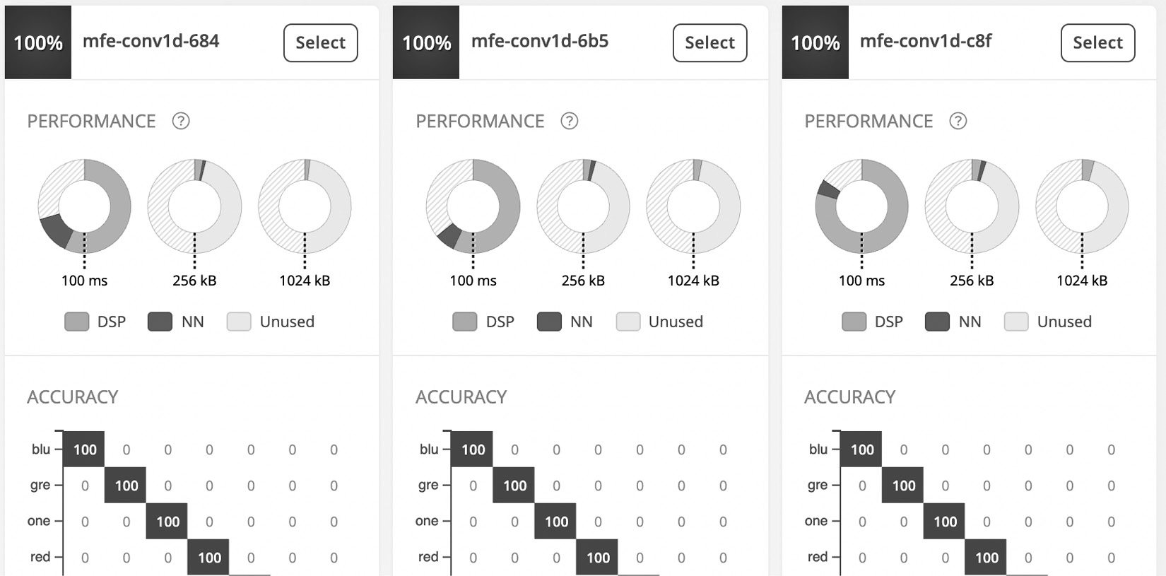
Figure 4.25 – EON Tuner reports a confusion matrix for each proposed ML solution

Once the EON Tuner has completed the discovery phase, you will have a collection of ML-based solutions (processing + ML model) to choose from.

4. Select an architecture with higher accuracy and lower window increase by clicking on the Select button. Our selected architecture has a 250-ms window increase and uses MFE as an input feature and 1D convolution layers.

As you can observe, the input feature is not MFCC. The EON Tuner proposes this alternative processing block because it considers the latency of the entire ML pipeline rather than just the model inference. Therefore, it is true that MFE could slow down the model inference because it returns a spectrogram with more features than MFCC. However, MFE is considerably faster than MFCC because it does not require extracting the DCT components.

Once you have selected an architecture, Edge Impulse will ask you to update the primary model. Click on Yes to override the architecture trained in the previous Designing and training a NN model recipe. A pop-up window will appear, confirming that the primary model has been updated.

In the end, click on Retrain model from the left-hand side panel and click on Train model to train the network again.

Live classifications with a smartphone

When we talk of model testing, we usually refer to the evaluation of the trained model on the testing dataset. However, model testing in Edge Impulse is more than that.

In this recipe, we will learn how to test model performance on the test set and show a way to perform live classifications with a smartphone.

Getting ready

Before implementing this recipe, the only thing we need to know is how we can evaluate model performance in Edge Impulse.

In Edge Impulse, we can evaluate the trained model in two ways:

• Model testing: We assess the accuracy using the test dataset. The test dataset provides an unbiased evaluation of model effectiveness because the samples are not used directly or indirectly during training.
• Live classification: This is a unique feature of Edge Impulse whereby we can record new samples either from a smartphone or a supported device (for example, the Arduino Nano).

The live classification approach benefits from testing the trained model in the real world before necessarily deploying the application on the target platform.

How to do it…

Follow the next steps to evaluate model performance with the test dataset and the live classification tool:

1. Click on Model testing from the left panel and click on Classify all.

Edge Impulse will take care of extracting the MFE from the test set, running the trained model, and reporting the performance in the confusion matrix.

2. Click on Live classification from the left panel and ensure the smartphone is reported in the Device list:

Figure 4.26 – Device list showing that the mobile phone is paired with Edge Impulse

Select Microphone from the Sensor drop-down list in the Live classification section and set the Sample length (ms) value to 10000. Keep Frequency at the default value (16000 Hz).

3. Click on Start sampling and then click on Give access to the Microphone on your phone. Record any of our six utterances (red, green, blue, one, two, and three). The audio sample will be uploaded on Edge Impulse once you have completed the recording.

At this point, Edge Impulse will split the recording into 1-second-length samples and test the trained model on each one. The classification results will be reported on the same page and in the following forms:

• Generic summary: This reports the number of detections for each output category:

Figure 4.27 – Generic summary reporting the number of detections for each keyword

• Detailed analysis: This reports the probability of the classes at each timestamp, as shown in the following screenshot:

Figure 4.28 – Detailed analysis reporting the probability of the classes at each timestamp

If you click on a table entry, Edge Impulse will show the corresponding audio waveform in the window, as shown in Figure 4.28.

Live classifications with the Arduino Nano

If you found live classification with the smartphone helpful, live classification with the Arduino Nano will be even more helpful.

This recipe will show how to pair the Arduino Nano with Edge Impulse to perform live classifications directly from our target platform.

Getting ready

Testing model performance with the sensor used in the final application is a good practice to have more confidence in the accuracy results. Thanks to Edge Impulse, it is possible to perform live classification on the Arduino Nano with a few simple steps that you can also find at the following link: https://docs.edgeimpulse.com/docs/arduino-nano-33-ble-sense.

How to do it…

Live classifications with the built-in microphone on the Arduino Nano require installing additional software on your machine. The different tools work on Linux, macOS, and Windows, and are listed here:

• Edge Impulse command-line interface (CLI): https://docs.edgeimpulse.com/docs/cli-installation
• Arduino CLI: https://arduino.github.io/arduino-cli/0.19/

Once you have installed the dependencies, follow the next steps to pair the Arduino Nano platform with Edge Impulse:

1. Run arduino-cli core install arduino:mbed_nano from Command Prompt or the terminal.
2. Connect the Arduino Nano board to your computer and press the RESET button on the platform twice to enter the device in bootloader mode.

The built-in LED should start blinking to confirm that the platform is in bootloader mode.

3. Download the Edge Impulse firmware for the Arduino Nano from https://cdn.edgeimpulse.com/firmware/arduino-nano-33-ble-sense.zip and decompress the file. The firmware will be required to send audio samples from the Arduino Nano to Edge Impulse.
4. In the unzipped folder, execute the flash script to upload the firmware on the Arduino Nano. You should use the script accordingly with your operating system (OS)—for example, flash_linux.sh for Linux.

Once the firmware has been uploaded on the Arduino Nano, you can press the RESET button to launch the program.

5. Execute edge-impulse-daemon from Command Prompt or the terminal. The wizard will ask you to log in and select the Edge Impulse project you're working on.

The Arduino Nano should now be paired with Edge Impulse. You can check if the Arduino Nano is paired by clicking on Devices from the left-hand side panel, as shown in the following screenshot:

Figure 4.29 – List of devices paired with Edge Impulse

As you can see from the preceding screenshot, the Arduino Nano (personal) is listed in the Your devices section.

Now, go to Live classification and select Arduino Nano 33 BLE Sense board from the Device drop-down list. You can now record audio samples from the Arduino Nano and check if the model works.

Important Note

If you discover that the model does not work as expected, we recommend adding audio samples recorded with the microphone of the Arduino Nano in the training dataset. To do so, click on Data acquisition and record new data using the Arduino Nano device from the right-hand side panel.

Continuous inferencing on the Arduino Nano

As you can guess, the application deployment differs on the Arduino Nano and the Raspberry Pi Pico because the devices have different hardware capabilities.

In this recipe, we will show how to implement a continuous keyword application on the Arduino Nano.

The following Arduino sketch contains the code referred to in this recipe:

• 07_kws_arduino_nano_ble33_sense.ino:

https://github.com/PacktPublishing/TinyML-Cookbook/blob/main/Chapter04/ArduinoSketches/07_kws_arduino_nano_ble33_sense.ino

Getting ready

The application on the Arduino Nano will be based on the nano_ble33_sense_microphone_continuous.cpp example provided by Edge Impulse, which implements a real-time KWS application. Before changing the code, we want to examine how this example works to get ready for the recipe.

Learning how a real-time KWS application works

A real-time KWS application—for example, the one used in the smart assistant—should capture and process all pieces of the audio stream to never miss any events. Therefore, the application needs to record the audio and run the inference simultaneously so that we do not skip any information.

On a microcontroller, parallel tasks can be performed in two ways:

• With a real-time OS (RTOS). In this case, we can use two threads for capturing and processing the audio data.
• With a dedicated peripheral such as direct memory access (DMA) attached to the ADC. DMA allows data transfer without interfering with the main program running on the processor.

In this recipe, we won't deal with this aspect directly. In fact, the nano_ble33_sense_microphone_continuous.cpp example already provides an application where the audio recording and inference run simultaneously through a double-buffering mechanism. Double buffering uses two buffers of fixed size, where the following applies:

• One buffer is dedicated to the audio sampling task.
• One buffer is dedicated to the processing task (feature extraction and ML inference).

Each buffer keeps the number of audio samples required for a window increase recording. Therefore, the buffer size can be calculated through the following formula:

The preceding formula can be defined as the product of the following:

• SF (Hz): Sampling frequency in Hz (for example, 16 kilohertz (kHz) = 16000 Hz)
• WI (s): Window increase in s (for example, 250 ms = 0.250 s)

For example, if we sample the audio signal at 16 kHz and the window increase is 250 ms, each buffer will have a capacity of 4,000 samples.

These two buffers are continuously switched between recording and processing tasks, and the following diagram visually shows how:

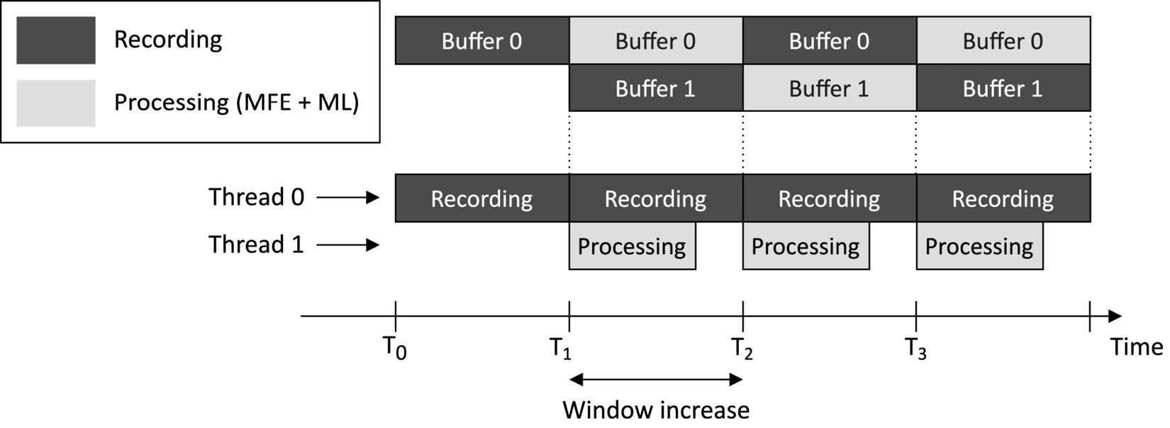
Figure 4.30 – Recording and processing tasks running simultaneously

From the preceding diagram, we can observe the following:

1. The recording task starts filling Buffer 0 at t=T0.
2. At t=T1, Buffer 0 is full. Therefore, the processing task can start the inference using the data in Buffer 0. Meanwhile, the recording task continues capturing audio data in the background using Buffer 1.
3. At t=T2, Buffer 1 is full. Therefore, the processing task must have finished the previous computation before starting a new one.

Keeping the window increase as short as possible has the following benefits:

• Increases the probability of getting the correct beginning of an utterance
• Reduces the computation time of feature extraction because this is only computed on the window increase

However, the window increase should be long enough to guarantee that the processing task can complete within this time frame.

At this point, you might have one question in mind: If we have a window increase of 250 ms, how can the double buffers feed the NN since the model expects a 1-s audio sample?

The double buffers are not the NN input but the input for an additional buffer containing the samples of the 1-s audio. This buffer stores the data on a first-in, first-out (FIFO) basis and provides the actual input to the ML model, as shown in the following diagram:

Figure 4.31 – The FIFO buffer is used to feed the NN model

Therefore, every time we start a new processing task, the sampled data is copied into the FIFO queue before running the inference.

How to do it…

With the following steps, we will make some changes to the nano_ble33_sense_microphone_continuous.cpp file to control the built-in RGB LEDs on the Arduino Nano with our voice:

1. In Edge Impulse, click on Deployment from the left-hand side menu and select Arduino Library from the Create library options, as shown in the following screenshot:

Figure 4.32 – Create library options in Edge Impulse

Next, click on the Build button at the bottom of the page and save the ZIP file on your machine. The ZIP file is an Arduino library containing the KWS application, the routines for feature extraction (MFCC and MFE), and a few ready-to-use examples for the Arduino Nano 33 BLE Sense board.

2. Open the Arduino integrated development environment (IDE) and import the library created by Edge Impulse. To do so, click on the Libraries tab from the left pane and then click on the Import button, as shown in the following screenshot:

Figure 4.33 – Import library in Arduino Web Editor

Once imported, open the nano_ble33_sense_microphone_continuous example from Examples | FROM LIBRARIES | <name_of_your_project>_INFERENCING.

In our case, <name_of_your_project> is VOICE_CONTROLLING_LEDS, which matches the name given to our Edge Impulse project.

In the file, the EI_CLASSIFIER_SLICES_PER_MODEL_WINDOW C macro defines the window increase in terms of the number of frames processed per model window. We can keep it at the default value.

3. Declare and initialize a global array of mbed::DigitalOut objects to drive the built-in RGB LEDs:

   mbed::DigitalOut rgb[] = {p24, p16, p6};

   #define ON 0

   #define OFF 1

The initialization of mbed::DigitalOut requires the PinName value of the RGB LEDs. The pin names can be found in the Arduino Nano 33 BLE Sense board schematic (https://content.arduino.cc/assets/NANO33BLE_V2.0_sch.pdf):

Figure 4.34 – The built-in RGB LEDs are powered by a current-sinking circuit (https://content.arduino.cc/assets/NANO33BLE_V2.0_sch.pdf)

The RGB LEDs—identified with the labels LR, LG, and LB—are controlled by a current-sinking circuit and are connected to P0.24, P0.16, and P0.06:

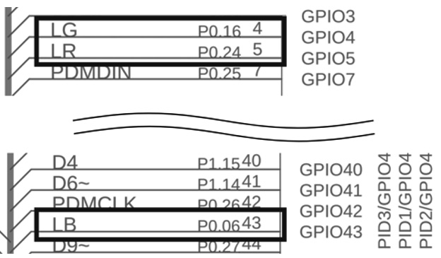
Figure 4.35 – The RGB LEDs are connected to P0.24, P0.16, and P0.06 (https://content.arduino.cc/assets/NANO33BLE_V2.0_sch.pdf)

Therefore, the general-purpose input/output (GPIO) pin must supply 0 volts (V) (LOW) to turn on the LEDs. To avoid using numerical values, we can use the #define ON 0 and #define OFF 1 C defines to turn the LEDs on and off.

4. Define an integer global variable (current_color) to keep track of the last detected color. Initialize it to 0 (red):

   size_t current_color = 0;

5. Initialize the built-in RGB LEDs in the setup() function by turning on just current_color:

   rgb[0] = OFF; rgb[1] = OFF; rgb[2] = OFF; rgb[current_color] = ON;

6. In the loop() function, set to false the moving average (MA) flag in the run_classifier_continuous() function:

   run_classifier_continuous(&signal, &result, debug_nn, false);

The run_classifier_continuous() function is responsible for the model inference. The MA is disabled by passing false after the debug_nn parameter. However, why do we disable this functionality?

MA is an effective method to filter out false detections when the window increase is small. For example, consider the word bluebird. This word contains blue, but it is not the utterance we want to recognize. However, when running continuous inference with a slight window increase, there is the benefit of processing small pieces of the word at a time. Therefore, the blue word may be detected with high confidence in one piece but not in the others. So, the goal of the MA is to average the results of classifications over time to avoid false detections.

As we can guess, the output class must have multiple high-rated classifications when using the MA. Therefore, what happens if the window increase is significant?

When the window increase is significant (for example, greater than 100 ms), we process fewer segments per second, and then the moving average could filter out all the classifications. Since our window increase will be between 250 ms and 500 ms (depending on the ML architecture chosen), we recommend you disable it to avoid filtering out the classifications.

7. Remove the code after run_classifier_continuous() till the end of the loop() function.
8. In the loop() function and after run_classifier_continuous(), write the code to return a class with higher probability:

   size_t ix_max = 0;

   float  pb_max = 0.0f;

   for (size_t ix = 0; ix < EI_CLASSIFIER_LABEL_COUNT; ix++) {

     if(result.classification[ix].value > pb_max) {

       ix_max = ix;

       pb_max = result.classification[ix].value;

     }

   }

In the preceding code snippet, we iterate through all the output classes (EI_CLASSIFIER_LABEL_COUNT) and keep the index (ix) with the maximum classification value (result.classification[ix].value). EI_CLASSIFIER_LABEL_COUNT is a C define provided by Edge Impulse and is equal to the number of output categories.

9. If the probability of the output category (pb_max) is higher than a fixed threshold (for example, 0.5) and the label is not unknown, check whether it is a color. If the label is a color and different from the last one detected, turn off current_color and turn on new_color:

   size_t new_color = ix_max;

   if (new_color != current_color) {

     rgb[current_color] = OFF;

     rgb[new_color] = ON;

     current_color = new_color;

   }

If the label is a number, blink the current_color LED for the recognized number of times:

const size_t num_blinks = ix_max0 - 2;

for(size_t i = 0; i < num_blinks; ++i) {

  rgb[current_color] = OFF;

  delay(1000);

  rgb[current_color] = ON;

  delay(1000);

}

Compile and upload the sketch on the Arduino Nano. You should now be able to change the color of the LED or make it blink with your voice.

Building the circuit with the Raspberry Pi Pico to voice control LEDs

The Raspberry Pi Pico has neither a microphone nor RGB LEDs onboard for building a KWS application. Therefore, voice controlling the RGB LEDs on this platform requires building an electronic circuit.

This recipe aims to prepare a circuit with the Raspberry Pi Pico, RGB LEDs, a push-button, and an electret microphone with a MAX9814 amplifier.

Getting ready

The application we have considered for the Raspberry Pi Pico is not based on continuous inferencing. Here, we would like to use a button to start the audio recording of 1 s and then run the model inference to recognize the utterance. The spoken word, in turn, will be used to control the status of the RGB LEDs.

In the following subsection, we will learn more about using the electret microphone with the MAX9814 amplifier.

Introducing the electret microphone amplifier with the MAX9814 amplifier

The microphone put into action in this recipe is the low-cost electret microphone amplifier – MAX9814. You can buy the microphone from the following distributors:

• Pimoroni: https://shop.pimoroni.com/products/adafruit-electret-microphone-amplifier-max9814-w-auto-gain-control
• Adafruit: https://www.adafruit.com/product/1713

The signal coming from the microphone is often tiny and requires amplification to be adequately captured and analyzed.

For this reason, our microphone is coupled with the MAX9814 chip (https://datasheets.maximintegrated.com/en/ds/MAX9814.pdf), an amplifier with built-in automatic gain control (AGC). AGC allows the capturing of speech in environments where the background audio level changes unpredictably. Therefore, the MAX9814 automatically adapts the amplification gain to make the voice always distinguishable.

The amplifier requires a supply voltage between 2.7V and 5.5V and produces an output with a maximum peak-to-peak voltage (Vpp) of 2Vpp on a 1.25V direct current (DC) bias.

Note

Vpp is the full height of the waveform.

Therefore, the device can be connected to ADC, expecting input signals between 0V and 3.3V.

As shown in the following diagram, the microphone module has five holes at the bottom for inserting the header strip:

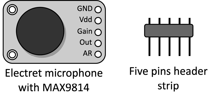
Figure 4.36 – Electret microphone with MAX9814

The header strip is required for mounting the device on the breadboard, and it typically needs to be soldered.

Tip

If you are not familiar with soldering, we recommend reading the following tutorial:

https://learn.adafruit.com/adafruit-agc-electret-microphone-amplifier-max9814/assembly

In the following subsection, you will discover how to connect this device with the Raspberry Pi Pico.

Connecting the microphone to the Raspberry Pi Pico ADC

The voltage variations produced by the microphone require conversion to a digital format.

The RP2040 microcontroller on the Raspberry Pi Pico has four ADCs to carry out this conversion, but only three of them can be used for external inputs because one is directly connected to the internal temperature sensor.

The pin reserved for the ADCs are shown here:

Figure 4.37 – ADC pins

The expected voltage range for the ADC on the Raspberry Pi Pico is between 0V and 3.3V, perfect for the signal coming from our electret microphone.

How to do it…

Let's start by placing the Raspberry Pi Pico on the breadboard. We should mount the platform vertically, as we did in Chapter 2, Prototyping with Microcontrollers.

Once you have placed the device on the breadboard, ensure the USB cable is not connected to power and follow the next steps to build the electronic circuit:

1. Place the RGB LEDs on the breadboard:

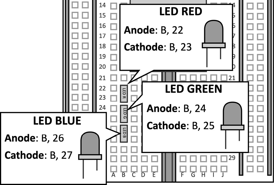
Figure 4.38 – RGB LEDs on the breadboard

Put the resistor in series to the LEDs by connecting one of the two terminals to the LED cathode and the other one to GND. The following table reports which resistor to use with each LED:

Figure 4.39 – Resistors used with the RGB LEDs

The resistances have been chosen to guarantee at least a ~3 milliampere (mA) forward current through each LED.

The following diagram shows how you can connect the resistors in series to the LEDs:

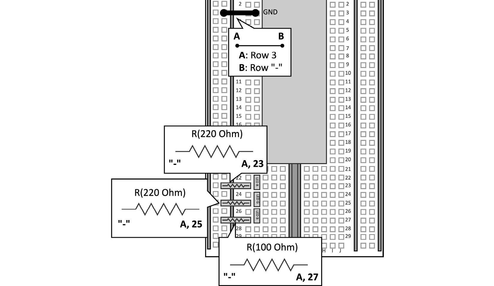
Figure 4.40 – Resistors in series to LEDs

As you can observe, you can plug the microcontroller's GND into the - rail to insert the resistor's terminal into the negative bus rail.

2. Connect the RGB LEDs' anode to the GPIO pins:

Figure 4.41 – Resistors connected to GND

As shown in the previous diagram, the GPIOs used to drive the LEDs are GP9 (red), GP8 (green), and GP7 (blue).

Since the resistor is connected between the LED cathode and GND, the LEDs are powered by a current sourcing circuit. Therefore, we should supply 3.3V (HIGH) to turn them on.

3. Place the push-button on the breadboard:

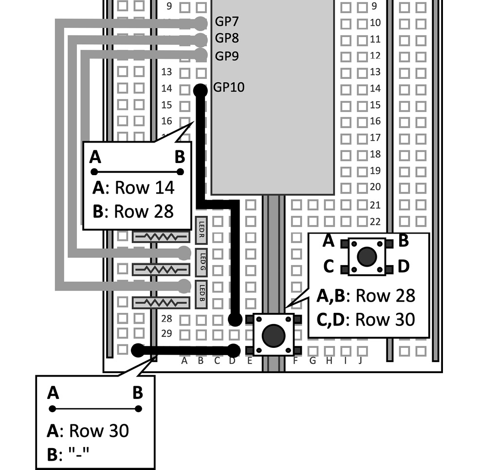
Figure 4.42 – Push-button connected to GP10 and GND

The GPIO used for the push-button is GP10.

Since our circuits will require several jumper wires, we place the device at the bottom of the breadboard to have enough space to press it.

4. Place the electret microphone on the breadboard:

Figure 4.43 – Electret microphone mounted on the breadboard

The ADC pin is GP26. Out of the five pins on the microphone module, we only need to connect three of them, which are outlined as follows:

• Vdd (3.3V): This is the supply voltage of the amplifier. Vdd must be stable and equal to the ADC supply voltage. These conditions are required to reduce the noise on the analog signal coming from the microphone.
• Vdd should be connected to ADC_VREF, the ADC reference voltage produced on the Raspberry Pi Pico.
• GND: This is the ground of the circuit amplifier and should be the same as the ADC peripheral. Since analog signals are more susceptible to noise than digital ones, the Raspberry Pi Pico offers a dedicated ground for ADCs: the analog ground (AGND). GND should be connected to AGND to decouple the analog circuit from the digital one.
• Out: This is the amplified analog signal coming from the microphone module and should be connected to GP26 to sample it with the ADC0 peripheral.

The following table reports the connections to make between the Raspberry Pi Pico and the electret microphone with the MAX9814 amplifier:

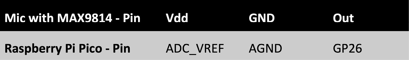
Figure 4.44 – Electret microphone connections

The remaining two terminals of the microphone are used to set the gain and the attach&release ratio. These settings are not required for this recipe, but you can discover more in the MAX9814 datasheet (https://datasheets.maximintegrated.com/en/ds/MAX9814.pdf).

At this point, you can plug the Raspberry Pi Pico into your computer through the Micro USB cable because the circuit is ready to implement our KWS application.

Audio sampling with ADC and timer interrupts on the Raspberry Pi Pico

All the components are now mounted on the breadboard. Therefore, there is nothing left for us to write our KWS application.

The application consists of recording 1-s audio and running the ML inference when pressing the push-button. The classification result will be shown through the RGB LEDs, similar to what we have done in the Continuous inferencing on the Arduino Nano recipe.

The following Arduino sketch and Python script contains the code referred to in this recipe:

• 09_kws_raspberrypi_pico.ino:

https://github.com/PacktPublishing/TinyML-Cookbook/blob/main/Chapter04/ArduinoSketches/09_kws_raspberrypi_pico.ino

• 09_debugging.py:

https://github.com/PacktPublishing/TinyML-Cookbook/blob/main/Chapter04/PythonScripts/09_debugging.py

Getting ready

The application on the Raspberry Pi Pico will be based on the Edge Impulse nano_ble33_sense_microphone.cpp example, where the user speaks at well-defined times and the application executes the ML model to guess the spoken word.

In contrast to what we implemented in the Continuous inferencing on the Arduino Nano recipe, the audio recording and processing task can be performed sequentially because the push-button will tell us the beginning of the utterance.

The following subsection will introduce the approach considered in this recipe to sample the audio signal with ADC and timer interrupts.

Audio sampling with ADC and timer interrupts on the Raspberry Pi Pico

The RP2040 microcontroller on the Raspberry Pi Pico has four ADCs with 12-bit resolution and a maximum sampling frequency of 500 kHz (or 500 kilosamples per second (kS/s)).

The ADC will be configured in one-shot mode, which means that the ADC will provide the sample as soon as we make the request.

The timer peripheral will be initialized to trigger interrupts at the same frequency as the sampling rate. Therefore, the interrupt service routine (ISR) will be responsible for sampling the signal coming from the microphone and storing the data in an audio buffer.

Since the ADC maximum frequency is 500 kHz, the minimum time between two consecutive conversions is 2 microseconds (us). This constraint is largely met because the audio signal is sampled at 16 kHz, which means every 62.5 us.

How to do it…

Open the nano_ble33_sense_microphone example from Examples | FROM LIBRARIES | <name_of_your_project>_INFERENCING, and make the following changes to implement the KWS application on the Raspberry Pi Pico:

1. Delete all the references to the PDM library, such as the header file (#include <PDM.h>) and calls to PDM class methods since these are only required for the built-in microphone of the Arduino Nano.

Remove the code within the microphone_inference_record() function.

2. Declare and initialize a global array of mbed::DigitalOut objects to drive the RGB LEDs:

   mbed::DigitalOut rgb[] = {p9, p8, p7};

Declare and initialize a global mbed::DigitalOut object to drive the built-in LED:

mbed::DigitalOut led_builtin(p25);

#define ON 1

#define OFF 0

Since a current sourcing circuit powers all LEDs, we need to supply 3.3V (HIGH) to turn them on.

3. Define an integer global variable (current_color) to keep track of the last detected color. Initialize it to 0 (red):

   size_t current_color = 0;

Initialize the RGB LEDs in the setup() function by turning on current_color only:

rgb[0] = OFF; rgb[1] = OFF; rgb[2] = OFF; rgb[current_color] = ON; led_builtin = OFF;

4. Declare and initialize the global mbed::DigitalIn object to read the push-button state:

   mbed::DigitalIn button(p10);

   #define PRESSED 0

Set the button mode to PullUp in the setup() function:

button.mode(PullUp);

Since the button is directly connected to GND and the GPIO pin, we must enable the internal pull-up resistor by enabling the PullUp button mode. Therefore, the numerical value returned by mbed::DigitalIn is 0 when the button is pressed.

5. Add the "hardware/adc.h" header file to use the ADC peripheral:

   #include "hardware/adc.h"

Initialize the ADC (GP26) peripheral in the setup() function using the Raspberry Pi Pico application programming interface (API):

adc_init(); adc_gpio_init(26); adc_select_input(0);

Raspberry Pi offers a dedicated API for the RP2040 microcontroller in the Raspberry Pi Pico SDK (https://raspberrypi.github.io/pico-sdk-doxygen/index.html).

Since the Raspberry Pi Pico SDK is integrated into the Arduino IDE, we don't need to import any library. We just need to include the header file ("hardware/adc.h") in the sketch to use the ADC's API.

The ADC is initialized by calling the following functions in setup():

1. adc_init(), to initialize the ADC peripheral.
2. adc_gpio_init(26), to initialize the GPIO used by the ADC. This function needs the GPIO pin number attached to the ADC peripheral. Therefore, we pass 26 because ADC0 is attached to GP26.
3. adc_select_input(0), to initialize the ADC input. The ADC input is the reference number of the ADC attached to the selected GPIO. Therefore, we pass 0 because we use ADC0.

By calling the preceding functions, we initialize the ADC in one-shot mode.

6. Declare a global mbed::Ticker object to use the timer peripheral:

   mbed::Ticker timer;

The timer object will be used to fire the timer interrupts at the frequency of the audio sampling rate (16 kHz).

7. Write the timer ISR to sample the audio coming from the microphone:

   #define BIAS_MIC ((int16_t)(1.25f * 4095) / 3.3f)

   volatile int  ix_buffer       = 0;

   volatile bool is_buffer_ready = false;

   void timer_ISR() {

     if(ix_buffer < EI_CLASSIFIER_RAW_SAMPLE_COUNT) {

       int16_t v = (int16_t)((adc_read() - BIAS_MIC));

       inference.buffer[ix_buffer] = v;

       ++ix_buffer;

     }

     else {

       is_buffer_ready = true;

     }

   }

The ISR samples the microphone's signal with the adc_read() function, which returns a value from 0 to 4096 because of the ADC resolution. Since the signal generated by the MAX9814 amplifier has a bias of 1.25V, we should subtract the corresponding digital sample from the measurement. The relationship between the voltage sample and the converted digital sample is provided with the following formula:

Here, the following applies:

• DS is the digital sample.
• resolution is the ADC resolution.
• VS is the voltage sample.
• VREF is the ADC supply voltage reference (for example, ADC_VREF).

Therefore, a 12-bit ADC with a VREF of 3.3V converts the 1.25V bias to 1552.

Once we have subtracted the bias from the measurement, we can store it in the audio buffer (inference.buffer[ix_buffer] = v) and then increment the buffer index (++ix_buffer).

The audio buffer needs to be dynamically allocated in setup() with microphone_inference_start(), and it can keep the number of samples required for a 1-s recording. The EI_CLASSIFIER_RAW_SAMPLE_COUNT C define is provided by Edge Impulse to know the number of samples in 1-s audio. Since we sample the audio stream with a sampling rate of 16 kHz, the audio buffer will contain 16,000 int16_t samples.

The ISR sets is_buffer_ready to true when the audio buffer is full (ix_buffer is greater than or equal to EI_CLASSIFIER_RAW_SAMPLE_COUNT).

ix_buffer and is_buffer_ready are global because they are used by the main program to know when the recording is ready. Since ISR changes these variables, we must declare them volatile to prevent compiler optimizations.

8. Write the code in microphone_inference_record() to record 1 s of audio:

   bool microphone_inference_record(void) {

     ix_buffer = 0;

     is_buffer_ready = false;

     led_builtin = ON;

     unsigned int sampling_period_us = 1000000 / 16000;

     timer.attach_us(&timer_ISR, sampling_period_us);

     while(!is_buffer_ready);

     timer.detach();

     led_builtin = OFF;

     return true;

   }

In microphone_inference_record(), we set ix_buffer to 0 and is_buffer_ready to false every time we start a new recording.

The user will know when the recording starts through the built-in LED light (led_builtin = ON).

At this point, we initialize the mbed::Ticker object to fire the interrupts with a frequency of 16 kHz. To do so, we call the attach_us() method, which requires the following:

• The ISR to call when the interrupt is triggered (&timer_ISR).
• The interval time for us to fire the interrupt. Since we sample the audio signal at 16 kHz, we pass 62us (unsigned int sampling_period_us = 1000000 / 16000).

The while(!is_buffer_ready) statement is used to check whether the audio recording is finished.

When the recording ends, we can stop generating the timer interrupts (timer.detach()) and turn off the built-in LED (led_builtin = OFF).

9. Check whether we are pressing the button in the loop() function:

   if(button == PRESSED) {

If so, wait for almost a second (for example, 700 ms) to avoid recording the mechanical sound of the pressed button:

  delay(700);

We recommend not releasing the push-button until the end of the recording to also prevent a mechanical sound when releasing it.

Next, record 1 s of audio with the microphone_inference_record() function and execute the model inference by calling run_classifier():

  microphone_inference_record();

  signal_t signal;

  signal.total_length = EI_CLASSIFIER_RAW_SAMPLE_COUNT;

  signal.get_data = &microphone_audio_signal_get_data;

  ei_impulse_result_t result = { 0 };

  run_classifier(&signal, &result, debug_nn);

After the run_classifier() function, you can use the same code written in the Continuous inferencing on the Arduino Nano recipe to control the RGB LEDs.

However, before ending the loop() function, wait for the button to be released:

  while(button == PRESSED);

}

Now, compile and upload the sketch on the Raspberry Pi Pico. When the device is ready, press the push-button, wait for the built-in LED light, and try to speak loud and close to the microphone to control the RGB LEDs with your voice.

You should now be able to control the RGB LEDs with your voice!

There's more…

What can we do if the application does not work? We may have different reasons, but one could be related to the recorded audio. For example, how can we know if the audio is recorded correctly?

To debug the application, we have implemented the 09_debugging.py Python script (https://github.com/PacktPublishing/TinyML-Cookbook/blob/main/Chapter04/PythonScripts/09_debugging.py) to generate an audio file (.wav) from the audio captured by the Raspberry Pi Pico.

The Python script works locally on your machine and only needs the PySerial, uuid, Struct, and Wave modules in your environment.

The following steps show how to use the Python script for debugging the application on the Raspberry Pi Pico:

1. Import the 09_kws_raspberrypi_pico.ino sketch (https://github.com/PacktPublishing/TinyML-Cookbook/blob/main/Chapter04/ArduinoSketches/09_kws_raspberrypi_pico.ino) in the Arduino IDE and set the debug_audio_raw variable to true. This flag will allow the Raspberry Pi Pico to transmit audio samples over the serial whenever we have a new recording.
2. Compile and upload the 09_kws_raspberrypi_pico.ino sketch on the Raspberry Pi Pico.
3. Run the 09_debugging.py Python script, providing the following input arguments:
   • --label: The label assigned to the recorded utterance. The label will be the prefix for the filename of the generated .wav audio files.
   • --port: Device name of the serial peripheral used by the Raspberry Pi Pico. The port's name depends on the OS—for example, /dev/ttyACM0 on GNU/Linux or COM1 on Windows. The easiest way to find out the serial port's name is from the device drop-down menu in the Arduino IDE:

Figure 4.45 – Device drop-down menu in Arduino Web Editor

Once the Python script has been executed, it will parse the audio samples transmitted over the serial to produce a .wav file whenever you press the push-button.

You can listen to the audio file with any software capable of opening .wav files.

If the audio level of the .wav file is too low, try speaking loud and close to the microphone when recording.

However, suppose the audio level is acceptable, and the application still does not work. In that case, the ML model is probably not generic enough to deal with the signal of the electret microphone. To fix this problem, you can expand the training dataset in Edge Impulse with the audio samples obtained from this microphone. For this scope, upload the generated .wav audio files in the Data acquisition section of Edge Impulse and train the model again. Once you have prepared the model, you just need to build a new Arduino library and import it into the Arduino IDE.

If you are wondering how this script works, don't worry. In the following chapter, you will learn more about it.