Chapter 1: Getting Started with TinyML

Here we are, with our first step into the world of TinyML.

This chapter starts with an overview of this emerging field, presenting the opportunities and challenges to bring machine learning (ML) to extremely low-power microcontrollers.

The body of this chapter focuses on the fundamental elements behind ML, power consumption, and microcontrollers that make TinyML unique and different from conventional ML in the cloud, desktops, or even smartphones. In particular, the Programming microcontrollers section will be crucial for those with little experience in embedded programming.

After introducing the TinyML building blocks, we shall set up the development environment for a simple LED application, which will officially mark the beginning of our practical TinyML journey.

In contrast to what we will find in the following chapters, this chapter has a more theoretical structure to get you familiar with the concepts and terminology of this fast-growing technology.

In this chapter, we're going to cover the following topics:

• Introducing TinyML
• Summary of deep learning
• Learning the difference between power and energy
• Programming microcontrollers
• Presenting Arduino Nano 33 BLE Sense and Raspberry Pi Pico
• Setting up Arduino Web Editor, TensorFlow, and Edge Impulse
• Running a sketch on Arduino Nano and Raspberry Pi Pico

Technical requirements

To complete the practical example in this chapter, we need the following:

• Arduino Nano 33 BLE Sense board
• Raspberry Pi Pico board
• Micro-USB cable
• Laptop/PC with either Ubuntu 18.04 or Windows 10 on x86-64

Introducing TinyML

Throughout all the recipes presented in this book, we will give practical solutions for tiny machine learning, or, as we will refer to it, TinyML. In this section, we will learn what TinyML is and the vast opportunities it brings.

What is TinyML?

TinyML is the set of technologies in ML and embedded systems to make use of smart applications on extremely low-power devices. Generally, these devices have limited memory and computational capabilities, but they can sense the physical environment through sensors and act based on the decisions taken by ML algorithms.

In TinyML, ML and the deployment platform are not just two independent entities but rather entities that need to know each other at best. In fact, designing an ML architecture without considering the target device characteristics will make it challenging to deploy effective and working TinyML applications.

On the other hand, it would be impossible to design power-efficient processors to expand the ML capabilities of these devices without knowing the software algorithms involved.

This book will consider microcontrollers as the target device for TinyML, and the following subsection will help motivate our choice.

Why ML on microcontrollers?

The first and foremost reason for choosing microcontrollers is their popularity in various fields, such as automotive, consumer electronics, kitchen appliances, healthcare, and telecommunications. Nowadays, microcontrollers are everywhere and also invisible in our day-to-day electronic devices.

With the rise of the internet of things (IoT), microcontrollers saw exponential market growth. In 2018, the market research company IDC (https://www.idc.com) reported 28.1 billion microcontrollers sold worldwide and forecasted growth to 38.2 billion by 2023 (www.arm.com/blogs/blueprint/tinyML). Those are impressive numbers considering that the smartphone and PC markets reported 1.5 billion and 67.2 million devices, respectively, sold in the same year.

Therefore, TinyML represents a significant step forward for IoT devices, driving the proliferation of tiny connected objects capable of performing ML tasks locally.

The second reason for choosing microcontrollers is that they are inexpensive, easy to program and are powerful enough to run sophisticated deep learning (DL) algorithms.

However, why can't we offload the computation to the cloud since it is much more performant? In other words, why do we need to run ML locally?

Why run ML locally?

There are three main answers to this question – latency, power consumption, and privacy:

• Reducing latency: Sending data back and forth to and from the cloud is not instant and could affect applications that must respond reliably within a time frame.
• Reducing power consumption: Sending and receiving data to and from the cloud is not power-efficient even when using low-power communication protocols such as Bluetooth.

In the following stacked bar chart, we report the power consumption breakdown for the onboard components on the Arduino Nano 33 BLE Sense board, one of the two microcontroller boards employed in this book:

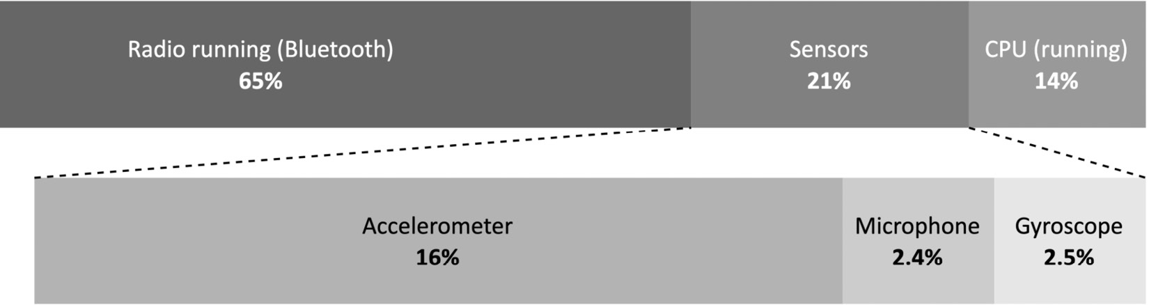
Figure 1.1 – Power consumption breakdown for the Arduino Nano 33 BLE Sense board

As we can see from the power consumption breakdown, the CPU computation is more power-efficient than Bluetooth communication (14% versus 65%), so it is preferable to compute more and transmit less to reduce the risk of rapid battery drain. Generally, radio is the component that consumes the most energy in typical embedded devices.

• Privacy: Local ML means preserving user privacy and avoiding sharing sensitive information.

Now that we know the benefits of running ML on these tiny devices, what are the practical opportunities and challenges of bringing ML to the very edge?

The opportunities and challenges for TinyML

TinyML finds its natural home wherever a power supply from the mains is impossible or complex to have, and the application must operate with a battery for as long as possible.

If we think about it, we are already surrounded by battery-powered devices that use ML under the hood. For example, wearable devices, such as smartwatches and fitness tracking bands, can recognize human activities to track our health goals or detect dangerous situations, such as a fall to the ground.

These everyday objects are TinyML applications for all intents and purposes because they are battery-powered and need on-device ML to give meaning to the data acquired by the sensors.

However, battery-powered solutions are not limited to wearable devices only. There are scenarios where we might need devices to monitor environments. For example, we may consider deploying battery-powered devices running ML in a forest to detect fires and prevent fires from spreading over a large area.

There are unlimited potential use cases for TinyML, and the ones we just briefly introduced are only a few of the likely application domains.

However, along with the opportunities, there are some critical challenges to face. The challenges are from the computational perspective because our devices are limited in memory and processing power. We work on systems with a few kilobytes of RAM and, in some cases, processors with no floating-point arithmetic acceleration.

On the other hand, the deployment environment could be unfriendly. Environmental factors, such as dust and extreme weather conditions, could get in the way and influence the correct execution of our applications.

In the following subsection, we will present the typical deployment environments for TinyML.

Deployment environments for TinyML

A TinyML application could live in both centralized and distributed systems.

In a centralized system, the application does not necessarily require communication with other devices.

A typical example is keyword spotting. Nowadays, we interact with our smartphones, cameras, drones, and kitchen appliances seamlessly with our voices. The magic words OK Google, Alexa, and so on that we use to wake up our smart assistants are a classic example of an ML model constantly running locally in the background. The application requires running on a low-power system without sending data to the cloud to be effective, instantly, and minimize power consumption.

Usually, centralized TinyML applications aim to trigger more power-hungry functionalities and benefit from being private by nature since they do not need to send any data to the cloud.

In a distributed system, the device (that is, the node or sensor node) still performs ML locally but also communicates with nearby devices or a host to achieve a common goal, as shown in the following figure:

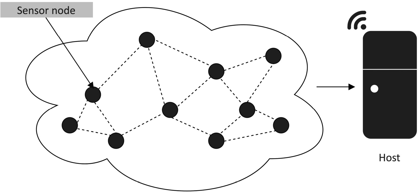
Figure 1.2 – Wireless sensor network

Important Note

Since the nodes are part of a network and typically communicate through wireless technologies, we commonly call the network a wireless sensor network (WSN).

Although this scenario could be contrasted with the power consumption implications of transmitting data, the devices may need to cooperate to build meaningful and precise knowledge about the working environment. Knowing the temperature, humidity, soil moisture, or other physical quantities from a specific node could be irrelevant for some applications that need a global understanding of the diffusion of those quantities instead.

For example, consider an application to improve agriculture efficiency. In this case, a WSN might help identify what areas of the field require less or more water than others and make the irrigation more efficient and autonomous. As we can imagine, efficient communication protocols will be vital for the network lifetime, and also TinyML plays a role in achieving this goal. Since sending raw data consumes too much energy, ML could perform a partial computation to reduce the data to transmit and the frequency

of communications.

TinyML offers endless possibilities, and tinyML Foundation is the best place to find out the endless opportunities given by this fast-growing field of ML and embedded systems.

tinyML Foundation

tinyML Foundation (www.tinyml.org) is a non-profit professional organization supporting and connecting the TinyML world.

To do this, tinyML Foundation, supported by several companies, including Arm, Edge Impulse, Google, and Qualcomm, is growing a diverse community worldwide (such as the US, UK, Germany, Italy, Nigeria, India, Japan, Australia, Chile, and Singapore) between hardware, software, system engineers, scientists, designers, product managers, and businesspeople.

The foundation has been promoting different free initiatives online and in-person to engage experts and newcomers to encourage knowledge sharing, connect, and create a healthier and more sustainable world with TinyML.

Tip

With several Meetup (https://www.meetup.com) groups in different countries, you can join a TinyML one near you for free (https://www.meetup.com/en-AU/pro/TinyML/) to always be up to date with new TinyML technologies and upcoming events.

After introducing TinyML, it is now time to explore its ingredients in more detail. The following section will analyze the one that makes our devices capable of intelligent decisions: DL.

Summary of DL

ML is the ingredient to make our tiny devices capable of making intelligent decisions. These software algorithms heavily rely on the right data to learn patterns or actions based on experience. As we commonly say, data is everything for ML because it is what makes or breaks an application.

This book will refer to DL as a specific class of ML that can perform complex classification tasks directly on raw images, text, or sound. These algorithms have state-of-the-art accuracy and could also be better than humans in some classification problems. This technology makes voice-controlled virtual assistants, facial recognition systems, and autonomous driving possible, just to name a few.

A complete discussion of DL architectures and algorithms is beyond the scope of this book. However, this section will summarize some of its essential points that are relevant to understand the following chapters.

Deep neural networks

A deep neural network consists of several stacked layers aimed at learning patterns.

Each layer contains several neurons, the fundamental compute elements for artificial neural networks (ANNs) inspired by the human brain.

A neuron produces a single output through a linear transformation, defined as the weighted sum of the inputs plus a constant value called bias, as shown in the following diagram:

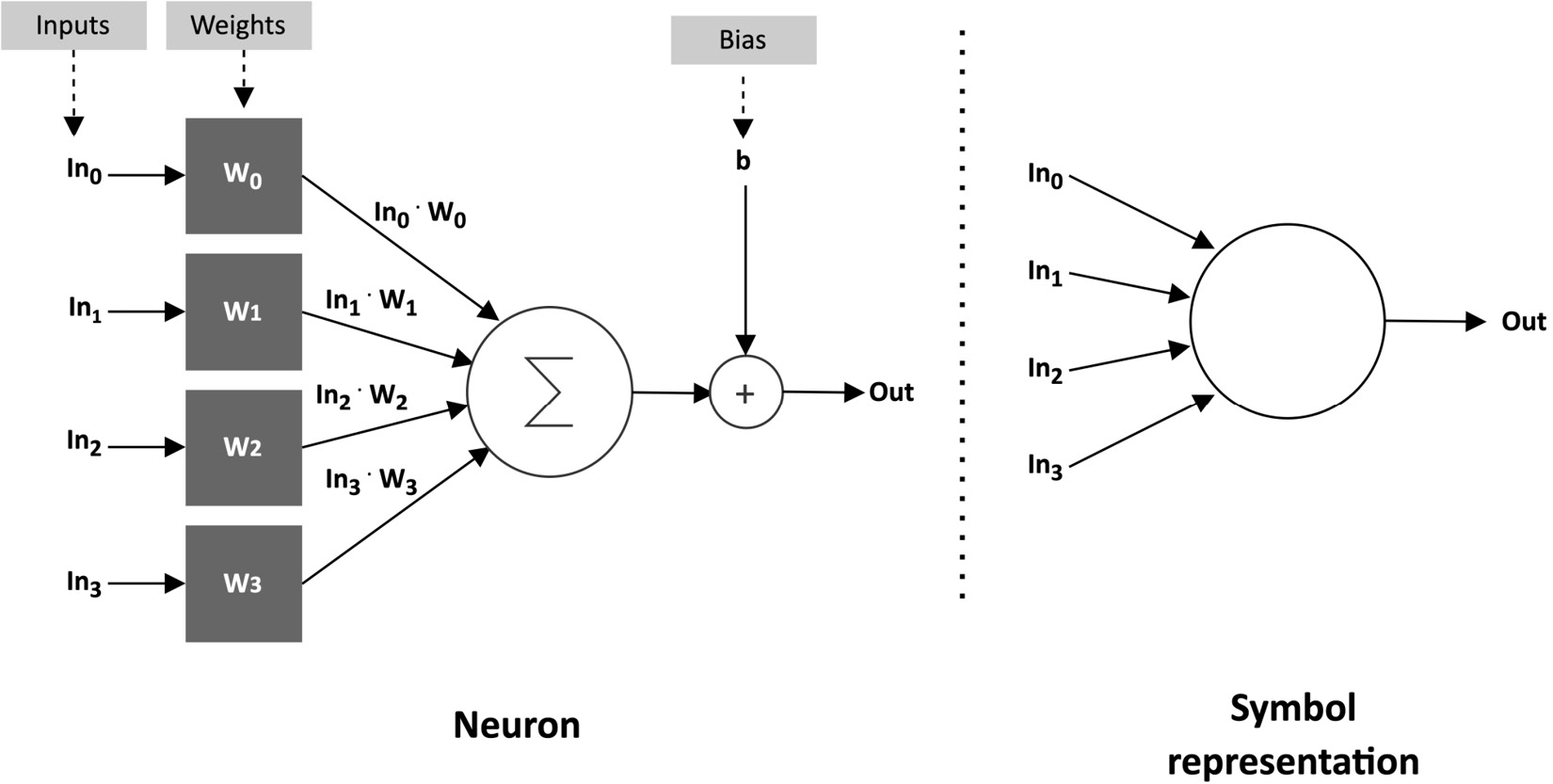
Figure 1.3 – Neuron representation

The coefficients of the weighted sum are called weights.

Weights and bias are obtained after an iterative training process to make the neuron capable of learning complex patterns.

However, neurons can only solve simple linear problems with linear transformations. Therefore, non-linear functions, called activations, generally follow the neuron's output to help the network learn complex patterns. Activation is a non-linear function performed on the neuron's output:

Figure 1.4 – Activation function

A widespread adopted activation function is the rectified linear unit (ReLU), described in the following code block:

float relu(float input) {

  return max(input, 0);

}

Its computational simplicity makes it preferable to other non-linear functions, such as a hyperbolic tangent or logistic sigmoid, that require more computational resources.

In the following subsection, we will see how the neurons are connected to solve complex visual recognition tasks.

Convolutional neural networks

Convolutional neural networks (CNNs) are specialized deep neural networks predominantly applied to visual recognition tasks.

We can consider CNNs as the evolution of a regularized version of the classic fully connected neural networks with dense layers (that is, fully connected layers).

As we can see in the following diagram, a characteristic of fully connected networks is connecting every neuron to all the output neurons of the previous layer:

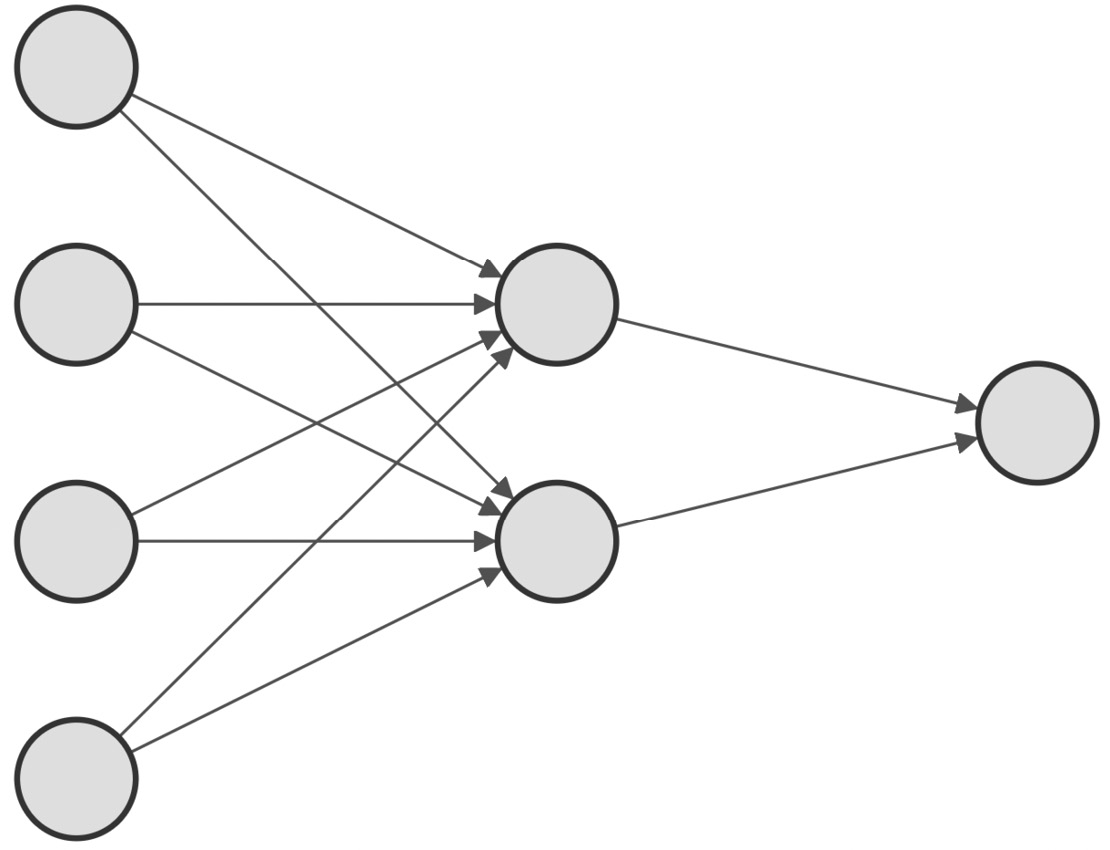
Figure 1.5 – Fully connected network

Unfortunately, this approach does not work well for training a model for image classification.

For instance, if we considered an RGB image of size 320x240 (width x height), we would need 230,400 (320*240*3) weights for just one neuron. Since our layers will undoubtedly need several neurons to discern complex problems, the model will likely overfit given the unmanageable number of trainable parameters.

In the past, data scientists adopted feature engineering techniques to extract a reduced set of good features from images. However, the approach suffered from being difficult to perform feature selection, which was time-consuming, and domain-specific.

With the rise of CNNs, visual recognition tasks saw improvement thanks to convolution layers that make feature extraction part of the learning problem.

Based on the assumption that we are dealing with images, and inspired by biological processes in the animal visual cortex, the convolution layer borrows the widely adopted convolution operator from image processing to create a set of learnable features.

The convolution operator is executed similarly to other image processing routines: sliding a window application (filter or kernel) on the entire input image and applying the dot product between its weights and the underlying pixels, as shown in the following figure:

Figure 1.6 – Convolution operator

This approach brings two significant benefits:

• It extracts the relevant features automatically without human intervention.
• It reduces the number of input signals per neuron considerably.

For instance, applying a 3x3 filter on the preceding RGB image would only require 27 weights (3*3*3).

Like fully connected layers, convolution layers need several convolution kernels to learn as many features as possible. Therefore, the convolution layer's output generally produces a set of images (feature maps), commonly kept in a multidimensional memory object called a tensor.

When designing CNNs for visual recognition tasks, we usually place the fully connected layers at the network's end to carry out the prediction stage. Since the output of the convolution layers is a set of images, typically, we adopt subsampling strategies to reduce the information propagated through the network and then reduce the risk of overfitting when feeding the fully connected layers.

Typically, there are two ways to perform subsampling:

• Skipping the convolution operator for some input pixels. As a result, the output of the convolution layer will have fewer spatial dimensions than the input ones.
• Adopting subsampling functions such as pooling layers.

The following figure shows a generic CNN architecture, where the pooling layer reduces the spatial dimensionality and the fully connected layer performs the classification stage:

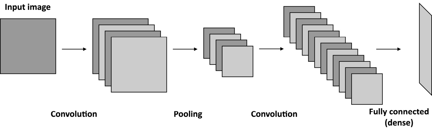
Figure 1.7 – Generic CNN with a pooling layer to reduce the spatial dimensionality

One of the most critical aspects to consider when deploying DL networks for TinyML is the model size, generally defined as the memory required for storing the weights.

Since our tiny platforms have limited physical memory, we require the model to be compact to fit the target device.

However, the memory constraint is not the only challenge we could encounter when deploying a model on microcontrollers. For example, although the trained model commonly employs arithmetic operations in floating-point precision, CPUs on microcontrollers could not have hardware acceleration for it.

Therefore, quantization is an indispensable technique to overcome the preceding limitations.

Quantization

Quantization is the process of performing neural network computations in lower bit precision. The widely adopted technique for microcontrollers applies the quantization post-training and converts the 32-bit floating-point weights to 8-bit integer values. This technique brings a 4x model size reduction and a significant latency improvement with very little or no accuracy drop.

DL is essential to building applications that make intelligent decisions. However, the key requirement for battery-powered applications is the adoption of a low-power device. So far, we have mentioned power and energy in general terms but let's see what they mean practically in the following section.

Learning the difference between power and energy

Power matters in TinyML, and the target we aim for is in the milliwatt (mW) range or below, which means thousands of times more efficient than a traditional desktop machine.

Although there are cases where we might consider using energy harvesting solutions, such as solar panels, those could not always be possible because of cost and physical dimensions.

However, what do we mean by power and energy? Let's discover these terms by giving a basic overview of the fundamental physical quantities governing electronic circuits.

Voltage versus current

Current is what makes an electronic circuit work, which is the flow of electric charges across surface A of a conductor in a given time, as described in the following diagram:

Figure 1.8 – Current is a flow of electric charges across surface A at a given time

The current is defined as follows:

Here, we have the following:

• I: Current, measured in amperes (A)
• Q: The electric charges across surface A in a given time, measured in coulombs (C)
• t: Time, measured in seconds (s)

The current flows in a circuit in the following conditions:

• We have a conductive material (for example, copper wire) to allow the electric charge to flow.
• We have a closed circuit, so a circuit without interruption, providing a continuous path to the current flow.
• We have a potential difference source, called voltage, defined as follows:

Voltage is measured with volts (V) and produces an electric field to allow the electric charge to flow in the circuit. Both the USB port and battery are potential difference sources.

The symbolic representation of a power source is given in the following figure:

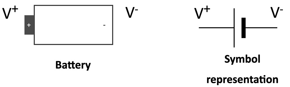
Figure 1.9 – Battery symbol representation

To avoid constantly referring to V+ and V-, we define the battery's negative terminal as a reference by convention, assigning it 0 V (GND).

Ohm's law relates voltage and current, which says through the following formula that the current through a conductor is proportional to the voltage across a resistor:

A resistor is an electrical component used to reduce the current flow. This component has a resistance measured with Ohm (Ω) and identified with the letter R.

The symbolic representation of a resistor is shown in the following figure:

Figure 1.10 – Resistor symbol representation (https://openclipart.org/detail/276048/47k-ohm-resistor)

Resistors are essential components for any electronic circuit, and for the ones used in this book, their value is reported through colored bands on the elements. Standard resistors have four, five, or six bands. The color on the bands denotes the resistance value, as shown in the following example:

Figure 1.11 – Example of four-band resistor

To easily decode the color bands, we recommend using the online tool from Digi-Key (https://www.digikey.com/en/resources/conversion-calculators/conversion-calculator-resistor-color-code).

Now that we know the main physical quantities governing electronic circuits, we are ready to see the difference between power and energy.

Power versus energy

Sometimes we interchange the words power and energy because we think they're related, but actually, they refer to different physical quantities. In fact, energy is the capacity for doing work (for example, using force to move an object), while power is the rate of consuming energy.

In practical terms, power tells us how fast we drain the battery, so high power implies a faster battery discharge.

Power and energy are related to voltage and current through the following formulas:

The following table presents the physical quantities in the power and energy formulas:

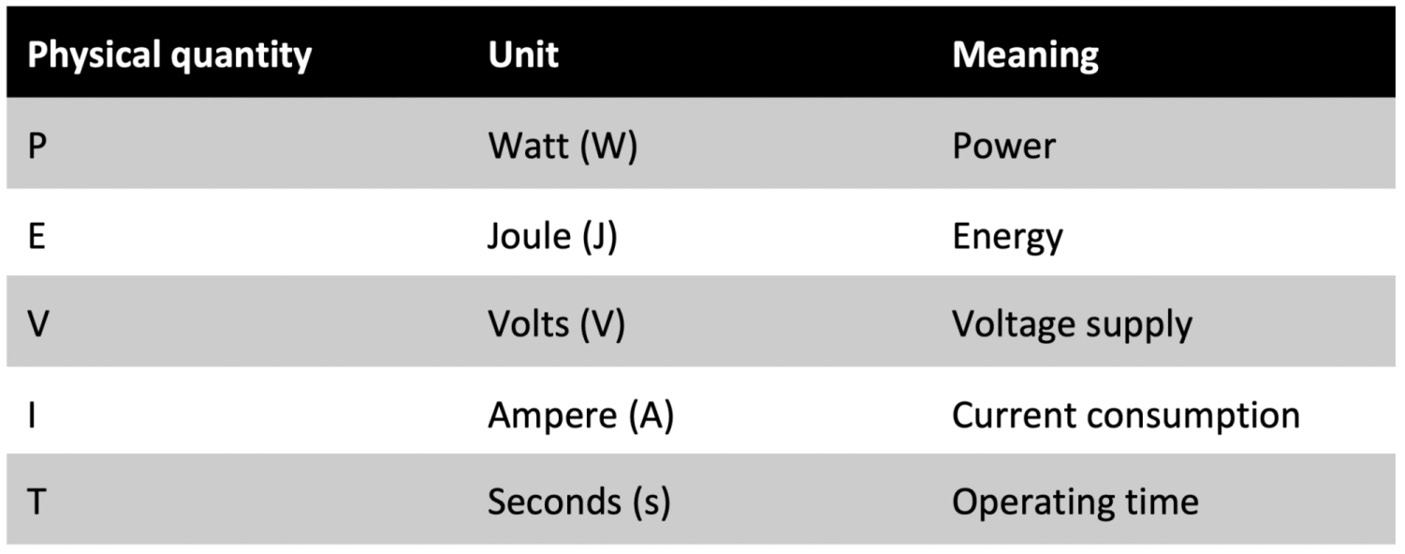
Figure 1.12 – Table reporting the physical quantities in the power and energy formulas

On microcontrollers, the voltage supply is in the order of a few volts (for example, 3.3 V), while the current consumption is in the range of micro-ampere (µA) or milli-ampere (mA). For this reason, we commonly adopt microwatt (µW) or milliwatt (mW) for power and microjoule (µJ) or millijoule (mJ) for energy.

Now, consider the following problem to get familiar with the power and energy concepts.

Suppose you have a processing task and you have the option to execute it on two different processors. These processors have the following power consumptions:

Figure 1.13 – Table reporting two processing units with different power consumptions

What processor would you use to execute the task?

Although PU1 has higher (4x) power consumption than PU2, this does not imply that PU1 is less energy-efficient. On the contrary, PU1 could be more computationally performant than PU2 (for example, 8x), making it the best choice from an energy perspective, as shown in the following formulas:

From the preceding example, we can say that PU1 is our better choice because it requires less energy from the battery under the same workload.

Commonly, we adopt OPS per Watt (arithmetic operations performed per Watt) to bind the power consumption to the computational resources of our processors.

Programming microcontrollers

A microcontroller, often shortened to MCU, is a full-fledged computer because it has a processor (which can also be multicore nowadays), a memory system (for example, RAM or ROM), and some peripherals. Unlike a standard computer, a microcontroller fits entirely on an integrated chip, and it has incredibly low power and low price.

We often confuse microcontrollers with microprocessors, but they refer to different devices. In contrast to a microcontroller, a microprocessor integrates only the processor on a chip, requiring external connections to a memory system and other components to form a fully operating computer.

The following figure summarizes the main differences between a microprocessor and a microcontroller:

Figure 1.14 – Microprocessor versus microcontroller

As for all processing units, the target application influences their architectural design choice.

For example, a microprocessor tackles scenarios where the tasks are usually as follows:

• Dynamic (for example, can change with user interaction or time)
• General-purpose
• Compute intensive

A microcontroller addresses completely different scenarios, and in the following list, we shall highlight some of the critical ones:

• The tasks are single-purpose and repetitive:

In contrast to microprocessor applications, the tasks are generally single-purpose and repetitive, so the microcontroller does not require strict re-programmability. Typically, the applications are less computationally intensive than the microprocessor ones and do not have frequent interactions with the user. However, they can interact with the environment or other devices.

As an example, you could consider a thermostat. The device only requires monitoring the temperature at regular intervals and communicating with the heating system.

• We could have time frame constraints:

Certain tasks must complete execution within a specific time frame. This requirement is the characteristic for real-time applications (RTAs), where the violation of the time constraint may affect the quality of service (soft real time) or be hazardous (hard real time).

An automobile safety system (ABS) is an example of a hard RTA because the electronic system must respond within a time frame to prevent the wheels from locking when applying brake pedal pressure.

We require a latency-predictable device to build an effective RTA, so all hardware components (CPU, memory, interrupt handler, and so on) must respond in a precise number of clock cycles. Hardware vendors commonly report the latency, expressed in clock cycles, in the datasheet.

The time constraint poses some architectural design adaptations and limitations to a general-purpose microprocessor.

An example is the memory management unit (MMU) that we primarily use to translate virtual memory addresses, and we do not usually have it in the CPU for microcontrollers.

• Low-power constraints:

Applications could live in a battery-powered environment, so the microcontroller must be low-power to extend their lifetime.

As per the time frame constraints, power consumption also poses some architectural design differences from a microprocessor.

Without going deeper into the hardware details, all the off-chip components generally reduce power efficiency as a rule of thumb. That is the main reason why microcontrollers integrate both the RAM and a kind of hard drive (ROM) within the chip.

Typically, microcontrollers also have lower clock frequency than microprocessors to consume less energy.

• Physical size constraints:

The device could live in products that are small in size. Since the microcontroller is a computer within a chip, it is perfect for these scenarios. The package size for a microcontroller can vary but typically is in the range of a few square millimeters.

In 2018, a team of engineers at the University of Michigan created the "world's smallest computer," which was 0.3 mm in size with a microcontroller powered by an Arm Cortex-M0+ processor and a battery-less sensor system for cellular temperature measurement (https://news.umich.edu/u-m-researchers-create-worlds-smallest-computer/).

• Cost constraints:

All applications are cost-sensitive, and by designing a smaller chip that integrates a CPU, memory, and peripherals, we make microcontrollers economically more advantageous than microprocessors.

In the following table, we have summarized what we have just discussed for easy future reference:

Figure 1.15 – Table comparing a microprocessor with a microcontroller

In the next section, we will start going deeper into the architectural aspects of microcontrollers by analyzing the memory architecture and internal peripherals.

Memory architecture

Microcontrollers are CPU-based embedded systems, which means that the CPU is responsible for interacting with all its subcomponents.

All CPUs require at least memory to read the instructions and store/read variables during the program's execution.

In the microcontroller context, we physically dedicate two separate memories for the instructions and data:

• Program memory (ROM)

This is non-volatile read-only memory reserved for the program to execute. Although its primary goal is to contain the program, it can also store constant data. Thus, program memory is similar to our everyday computers' hard drives.

• Data memory (RAM)

This is volatile memory reserved to store/read temporary data. Since it is RAM, we lose its content when switching off the system.

Since program and data memory are functionally opposite, we usually employ different semiconductor technologies. In particular, we can find Flash technologies for the program memory and static random-access memory (SRAM) for the data memory.

Flash memories are non-volatile and offer low power consumption but are generally slower than SRAM. However, given the cost advantage over SRAM, we can find larger program memory than data memory.

Now that we know the difference between program and data memory, where can we store the weights for our deep neural network model?

The answer to this question depends on whether the model has constant weights. If the weights are constant, so do not change during inference, it is more efficient to store them in program memory for the following reasons:

• Program memory has more capacity than SRAM.
• It reduces memory pressure on the SRAM since other functions require storing variables or chunks of memory at runtime.

We want to remind you that microcontrollers have limited memory resources, so a decision like this can make a difference to memory efficiency.

Peripherals

Microcontrollers offer extra on-chip features to expand their capabilities and make these tiny computers different from each other. These features are the peripherals and are essential because they can interface with sensors or other external components.

Each peripheral has a dedicated functionality, and it is assigned to a metal leg (pin) of the integrated circuit.

We can refer to the peripheral pin assignment section in the microcontroller datasheet to find out each pin's functionalities. Hardware vendors typically number the pins anti-clockwise, starting from the top-left corner of the chip, marked with a dot for easy reference, as shown in the following figure:

Figure 1.16 – Pin assignment. Pins are numbered anti-clockwise, starting from the top-left corner, marked with a dot

Since peripherals can be of various types, we can group them into four main categories for simplicity.

General-purpose input/output (GPIO or IO)

GPIOs do not have a predefined and fixed purpose. Their primary function is to provide or read binary signals that, by nature, can only live in two well-defined states: HIGH (1) or LOW (0). The following figure shows an example of a binary signal:

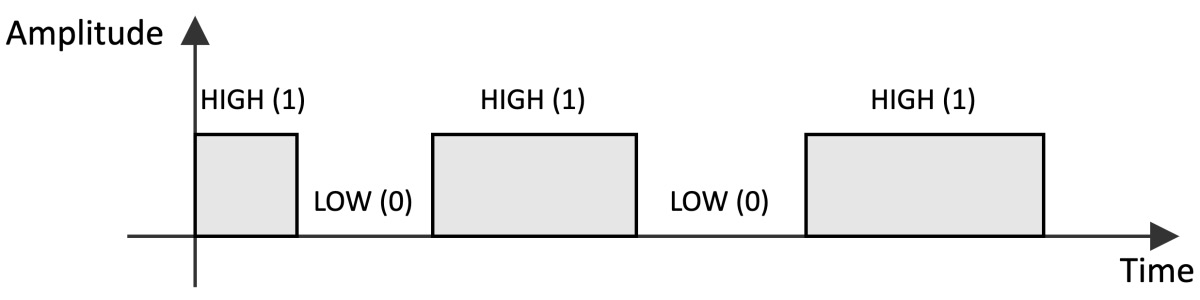
Figure 1.17 – A binary signal can only live in two states: HIGH (1) and LOW (0)

Typical GPIO usages are as follows:

• Turning on and off an LED
• Detecting whether a button is pressed
• Implementing complex digital interfaces/protocols such as VGA

GPIO peripherals are versatile and generally available in all microcontrollers.

Analog/digital converters

In TinyML, our applications will likely be dealing with time-varying physical quantities, such as images, audio, and temperature.

Whatever these quantities are, the sensor transforms them into a continuous electrical signal interpretable by the microcontrollers. This electrical signal, which can be either a voltage or current, is commonly called an analog signal.

The microcontroller, in turn, needs to convert the analog signal into a digital format so that the CPU can process the data.

Analog/digital converters act as translators between analog and digital worlds.

An analog-to-digital converter (ADC) samples the analog signal at fixed interval times and converts the electrical signal into a digital format.

A digital-to-analog converter (DAC) performs the opposite functionality: converting the internal digital format into an analog signal.

Serial communication

Communication peripherals integrate standard communication protocols to control external components. Typical serial communication peripherals available in microcontrollers are I2C, SPI, UART, and USB.

Timers

In contrast to all the peripherals we just described, the timers do not interface with external components since they are used to trigger or synchronize events.

With this section, we have completed the overview of the TinyML ingredients. Now that we are familiar with the terminology and general concepts, we can start presenting the development platforms used in this book.

Presenting Arduino Nano 33 BLE Sense and Raspberry Pi Pico

A microcontroller board is a printed circuit board (PCB) that combines the microcontroller with the necessary electronic circuit to make it ready to use. In some cases, the microcontroller board could integrate additional devices to target specific end applications.

Arduino Nano 33 BLE Sense (in short, Arduino Nano) and Raspberry Pico are the microcontroller boards used in this book.

Arduino Nano, designed by Arduino (https://www.arduino.cc), is a board that combines a microcontroller (nRF52840) powered by an Arm Cortex-M4 processor with several sensors and Bluetooth radio for an easy TinyML development experience. We will require just a few additional external components when developing on Arduino Nano since most are already available on-board.

Raspberry Pi Pico, designed by the Raspberry Pi Foundation (https://www.raspberrypi.org), does not provide sensors and the Bluetooth module on-board. Still, it has a microcontroller (RP2040) powered by a dual-core Arm Cortex-M0+ processor for unique and powerful TinyML applications. Therefore, this board will be ideal for learning how to interface with external sensors and build electronic circuits.

The following figure shows a side-by-side comparison to see the features that make our platforms different from each other:

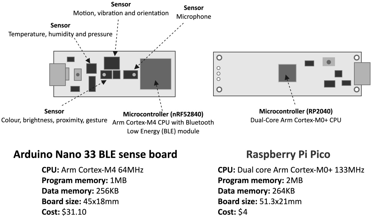
Figure 1.18 – Arduino Nano 33 BLE Sense versus Raspberry Pi Pico

As we can see from the side-by-side comparison, they both have an incredibly small form-factor, a USB port for power/programming, and an Arm-based microcontroller. At the same time, they also have unique features that make the boards ideal for targeting different TinyML development scenarios.

Setting up Arduino Web Editor, TensorFlow, and Edge Impulse

For TinyML, we require different software tools to cover both ML development and embedded programming. Thanks to Arduino, Edge Impulse, and Google, most of the tools considered in this book are browser-based and require only a few configuration steps.

In this section, we will introduce these tools and prepare the Arduino development environment required for writing and uploading programs to Arduino Nano and Raspberry Pi Pico.

Getting ready with Arduino Web Editor

Arduino Integrated Development Environment (Arduino IDE) is a software application developed by Arduino (https://www.arduino.cc/en/software) for writing and uploading programs to Arduino-compatible boards. Programs are written in C++ and are commonly called sketches by Arduino programmers.

Arduino IDE makes software development accessible and straightforward to developers with no background in embedded programming. In fact, the tool hides all the complexities that we might have when dealing with embedded platforms, such as cross-compilation and device programming.

Arduino also offers a browser-based IDE (https://create.arduino.cc/editor). It is called Arduino Web Editor and makes programmability even more straightforward because programs can be written, compiled, and uploaded on microcontrollers directly from the web browser. All the Arduino projects presented in this book will be based on this cloud-based environment. However, since the free plan of Arduino Web Editor is limited to 200 seconds of compilation time per day, you may consider upgrading to a paid plan or using the free local Arduino IDE to get unlimited compilation time.

Note

In the following chapters of this book, we will use Arduino IDE and Arduino Web Editor interchangeably.

Getting ready with TensorFlow

TensorFlow (https://www.tensorflow.org) is an end-to-end free and open source software platform developed by Google for ML. We will be using this software to develop and train our ML models using Python in Google Colaboratory.

Colaboratory (https://colab.research.google.com/notebooks), in short, Colab, is a free Python development environment that runs in the browser using Google Cloud. It is like a Jupyter notebook but has some essential differences, such as the following:

• It does not need setting up.
• It is cloud-based and hosted by Google.
• There are numerous Python libraries pre-installed (including TensorFlow).
• It is integrated with Google Drive.
• It offers free access to GPU and TPU shared resources.
• It is easy to share (also on GitHub).

Therefore, TensorFlow does not require setting up because Colab comes with it.

In Colab, we recommend enabling the GPU acceleration on the Runtime tab to speed up the computation on TensorFlow. To do so, navigate to Runtime | Change runtime type and select GPU from the Hardware accelerator drop-down list, as shown in the following screenshot:

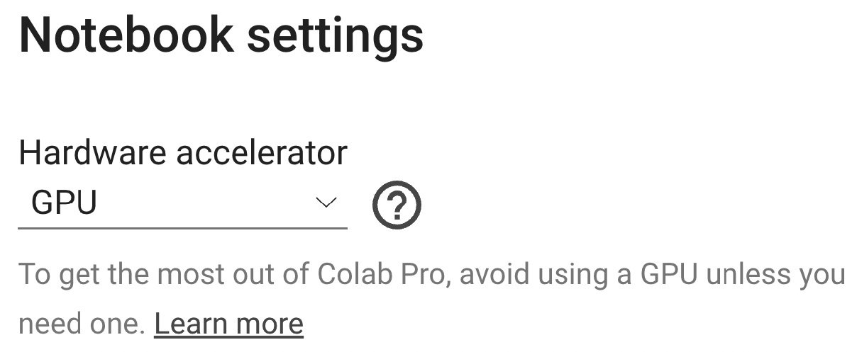
Figure 1.19 – You can enable the GPU acceleration from Runtime | Change runtime type

Since the GPU acceleration is a shared resource among other users, there is limited access to the free version of Colab.

Tip

You could subscribe to Colab Pro (https://colab.research.google.com/) to get priority access to the fastest GPUs.

TensorFlow is not the only tool from Google that we will use. In fact, once we have produced the ML model, we will need to run it on the microcontroller. For this, Google developed TensorFlow Lite for Microcontrollers.

TensorFlow Lite for Microcontrollers (https://www.tensorflow.org/lite/microcontrollers), in short, TFLu, is the key software library to unlock ML applications on low-power microcontrollers. The project is part of TensorFlow and allows running DL models on devices with a few kilobytes of memory. Written in C/C++, the library does not require an operating system and dynamic memory allocation.

TFLu does not need setting up because it is included in Arduino Web Editor.

Getting ready with Edge Impulse

Edge Impulse (https://www.edgeimpulse.com) is a software platform for end-to-end ML development. It is free for developers, and in a few minutes, we can 
have an ML model up and running on our microcontrollers. In fact, the platform integrates tools for the following:

• Data acquisition from sensor data
• Applying digital signal processing routines on input data
• Building and training ML models
• Testing ML models
• Deploying ML models on microcontrollers
• Finding the best signal processing block and ML model for your use case

  Info

  All these tools are also accessible through open APIs.

Developers just need to sign up on the website to access all these features directly within the UI.

How to do it…

The following subsections will show the steps for setting up Arduino Web Editor:

1. Sign up to Arduino at https://auth.arduino.cc/register.
2. Log in to Arduino Web Editor (https://create.arduino.cc/editor).
3. Install the Arduino agent following the step-by-step installation at https://create.arduino.cc/getting-started/plugin/welcome.
4. Install the Raspberry Pi Pico SDK:
   • Windows:
     1. Download the pico-setup-windows file from https://github.com/ndabas/pico-setup-windows/releases.
     2. Install pico-setup-installer.
   • Linux:
     1. Open Terminal.
     2. Create a temporary folder:

     $ mkdir tmp_pico

   3. Change directory to your temporary folder:

   $ cd tmp_pico

   4. Download the Pico setup script with wget:

   $ wget wget https: //raw.githubusercontent.com/raspberrypi/ pico-setup/master/pico_setup.sh

   5. Make the file executable:

   $ chmod +x pico_setup.sh

   6. Execute the script:

   $ ./pico_setup.sh

   7. Add $USER to the dialout group:

   $ sudo usermod -a -G dialout $USER

5. Check whether Arduino Web Editor can communicate with Arduino Nano:
   1. Open Arduino Web Editor in a web browser.
   2. Connect the Arduino Nano board to a laptop/PC through a micro-USB cable.

The editor should recognize the board in the device dropdown and report Arduino Nano 33 BLE and the port's name (for example, /dev/ttyACM0):

Figure 1.20 – Expected output when Arduino Web Editor can communicate with Arduino Nano

6. Check whether Arduino Web Editor can communicate with Raspberry Pi Pico:
   1. Open Arduino Web Editor in a browser.
   2. Connect the Raspberry Pi Pico board to a laptop/PC through a micro-USB cable.

The editor should recognize the board and report Raspberry Pi Pico and the port's name (for example, /dev/ttyACM0):

Figure 1.21 – Expected output when Arduino Web Editor can communicate with Raspberry Pi Pico

We have successfully set up the tools that will help us develop our future recipes. Before ending this chapter, we want to test a basic example on Arduino Nano and Raspberry Pi Pico to officially mark the beginning of our journey into the world of TinyML.

Running a sketch on Arduino Nano and Raspberry Pi Pico

In this recipe, we will blink the Arduino Nano and Raspberry Pi Pico LED using the Blink prebuilt example from Arduino Web Editor.

This "Hello World" program consists of a simple LED blinking through the GPIO peripheral; from there, we will be able to go anywhere.

This exercise aims to get you familiar with Arduino Web Editor and help you to understand how to develop a program with Arduino.

Getting ready

An Arduino sketch consists of two functions, setup() and loop(), as shown in the following code block:

void setup() {

}

void loop() {

}

setup() is the first function executed by the program when we press the reset button or power up the board. This function is executed only once and is generally responsible for initializing variables and peripherals.

After setup(), the program executes loop(), which runs iteratively and forever, as shown in the following figure:

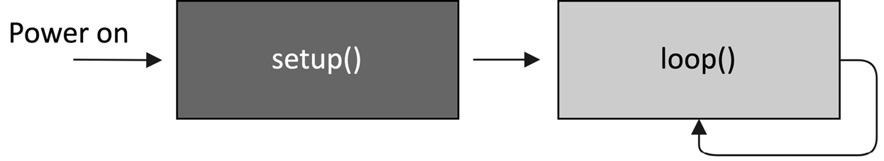
Figure 1.22 – Diagram of the structure

These two functions are required in all Arduino programs.

How to do it…

The steps reported in this section are valid for both Arduino Nano, Raspberry Pi Pico, and other compatible boards with Arduino Web Editor:

1. Connect the device to a laptop/PC through a micro-USB cable. Next, check that the Arduino IDE reports the name and port for the device.
2. Open the prebuilt Blink example by clicking on Examples from the left-hand side menu, BUILT IN from the new menu, and then Blink, as shown in the following screenshot:

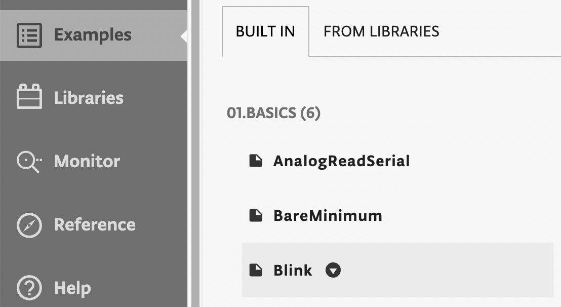
Figure 1.23 – Built-in LED blink example

Once you have clicked on the Blink sketch, the code will be visible in the editor area.

3. Click on the arrow near the board dropdown to compile and upload the program to the target device, as shown in the following figure:

Figure 1.24 – The arrow near the board dropdown will compile and flash the program on the target device

The console output should return Done at the bottom of the page, and the on-board LED should start blinking.

Join us on Discord!

Read this book alongside other users, TinyML developers/engineers and Gian. Ask questions, provide solutions to other readers, chat with the Gian via Ask Me Anything sessions and much more.

Join Now!

https://discord.com/invite/UCJTV3A2Qp