The Bayes factor is a metric used to decide between two competing models that describe a process: in our case, a predictive algorithm. I demonstrate how a Bayes factor can be used to decide whether a sophisticated algorithm outperforms a Naive algorithm that simply predicts the most common label.
Let M1 and M2 be two competing models. M1 is likely to be the model we are considering replacing M2, and a larger K indicates more evidence that M1 is the better model. If M1 denotes our predictive algorithm, a large K indicates that our algorithm does a good job of predicting the target variable.
Now recall that, in Bayesian statistics, we have a prior distribution, we collect data, and we compute a posterior distribution for an event. Here, the event of interest will be whether a certain model is appropriate. M1 is the event that our table-lookup algorithm does a better job than the naive algorithm, while M2 is the event that the naive algorithm is better than our table-lookup algorithm. Let p1 denote the accuracy of the table-lookup algorithm, and p2 the accuracy of the naive algorithm. M1 corresponds to the event that p1 is greater than p2, while M2 corresponds to the event that p1 is less than p2. So, we're going to use conjugate priors, like we did in Chapter 1, Classical Statistical Analysis.
We're going to assume that these two parameters, which are like random variables, are independent under this prior distribution. We're also going to use the B(3,3) distribution for our prior for both of these. Now, I'm not going to explain why, but it's not that hard to show that these assumptions lead to the prior probabilities for both M1 and M2 being 1/2, and this is not necessarily true in general. So, what does that mean? It means that this factor is going to be canceled out and just turn into 1.
So, let's go ahead and compute a Bayes factor:
- You may remember that we need the number of successes and the total sample size in order to compute the posterior distribution's parameters. Here, I compute those parameters:

- Now, we will see the posterior distribution of the parameters for the lookup algorithm's accuracy:

- Now, let's do the same thing for the naive algorithm. We will generate the values as follows:

Here are the number of individuals who died and the number of individuals who survived the disaster. The naive algorithm predicts that everybody died. 62 is the number of correct predictions, and 27 is the number of incorrect predictions.
- We will compute the parameters for the posterior distribution as follows:

We end up with these parameters for the posterior distribution of the accuracy of the naive algorithm.
- Once again, it's pretty difficult to explicitly compute this probability. So, we are going to use the simulation trick that we looked at in Chapter 1, Classical Statistical Analysis, to estimate the probability that p1 is less than p2, as follows:
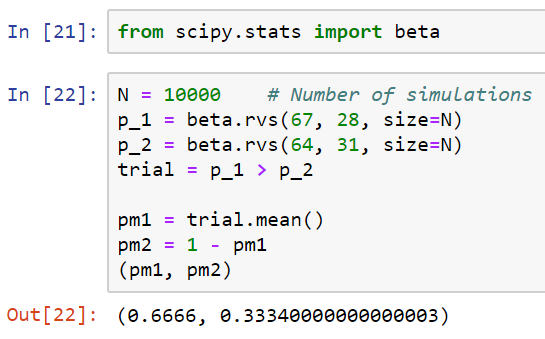
There's a 68% chance that M1 is appropriate—the model that says that our new algorithm does a better job than the naive algorithm—and a 32% chance that that is not true.
- So now, we can use this to compute the Bayes factor:
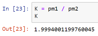
So, what do we make of this number? Well, we have what's called the Jeffreys' scale to give an interpretation to the Bayes factor that we computed, which is as follows:
| K | Strength of evidence |
| >1 | Evidence for M2 |
| 1 to 101/2 (≈3.2) | Negligible |
| 101/2 to 10 | Substantial |
| 10 to 103/2 (≈31.6) | Strong |
| 103/2 to 100 | Very strong |
| >100 | Decisive |
Our K falls into the negligible range. Our algorithm seems to do barely better than the naive algorithm at predicting who survived the Titanic, and is not worth the computational effort.