
C H A P T E R 9
SQL Server Analysis Services
In the previous chapter, you saw how aggregation queries, such as counts and sums, can have a significant adverse impact on the performance of a database. The problems arise partly because of the time it takes the relational database to step through each row in the tables involved and partly because of an increase in memory use. If the aggregation requires scanning a large table or index, the process can displace other buffers from memory so that SQL Server has to read them from disk again the next time another query needs them.
One way to improve the performance of aggregation queries is to cache their results. You can make the cached results available to all the servers in your web tier by using a small database table for your cache. Imagine that you have many different kinds of aggregations that you would like to cache, over a variety of parameters. If you were to take that concept and expand on it considerably, you would eventually find that you need a way to query the cached data and to update it regularly and that it’s possible to gain some powerful insights into your data that way. This realization resulted in the creation of the first multidimensional databases (MDDBs) and eventually an entire industry known as business intelligence (BI). SQL Server Analysis Services (SSAS) is Microsoft’s BI product. It comes “in the box” with the commercial and developer versions of Microsoft’s relational database (not with SQL Express).
Although BI seems to be used most often to support back-end reporting, it can also play an important role in improving the performance of your web tier. You can move aggregation queries to SSAS and eliminate their adverse performance impact on your relational database. Not only should the aggregation queries themselves run faster, but the rest of your RDBMS should also run faster because buffering efficiency improves and the load on your disk subsystem declines.
Communication about BI and data warehousing unfortunately is often made confusing because of a conflicting use of a plethora of industry-specific terms by companies, books, and individuals. I've endeavored to reduce confusion here by listing these terms and definitions as I use them in the glossary. Even if you’ve worked with BI before, I encourage you to review the glossary.
This chapter starts with a summary of how SSAS works and how you can use it in your web site. You then walk through a detailed example that involves building a cube and issuing queries against it from a web page.
Analysis Services Overview
The term multidimensional is used when talking about BI because the technology allows you to look at aggregations from several different directions. If you had a table of past order details, you might want to look at things such as the number of orders by date, the number of orders by customer, dollars by customer, or dollars by state the customer lives in. Each of these different views through your data is called a slice.
A collection of aggregations is called a cube. A cube is the multidimensional equivalent of a single relational database management system (RDBMS); a cube contains facts and dimensions, whereas an RDBMS contains tables. A collection of cubes is called a multidimensional database (MDDB). When you add an SSAS project to Visual Studio, you are adding an MDDB.
SSAS retrieves the data that it uses for its calculations from an RDBMS. To do that, first you define a data source that contains instructions about how to connect to your database. Then, you define a Data Source View (DSV) that tells SSAS how the tables in your database are associated with each other. With the DSV in place, you can define and build a cube. When you define a cube, you specify which tables contain facts, which are collections of numeric information and foreign keys. You also specify which tables contain dimensions, which are collections of primary keys and strings (usually). At first, a cube contains only some high-level precomputed aggregations. As you place queries against the cube, SSAS caches any new aggregations that it has to calculate. You can also configure your cube to precompute a larger number of aggregations up front.
After you’ve defined a cube in Visual Studio, you need to deploy it to the server before you can place queries against it. After deployment, SSAS may need to reaggregate the associated data through processing. Using proactive caching, you can automate processing so that it happens either periodically or when data changes. You can also request reprocessing from Visual Studio or SQL Server Integration Services (SSIS).
After you have deployed and processed a cube, you can issue queries against it. Visual Studio contains a data browser that supports an easy drag-and-drop query interface you can use for testing. For reporting, data browsing, or testing purposes, you can also use pivot tables in Excel to browse the cube, or you can view its structure with pivot diagrams in Visio. In addition, SQL Server Reporting Services (SSRS) can query the cube and generate reports from the results.
You can use SQL Server Management Studio (SSMS) to interface to SSAS; instead of connecting to a relational database, you can connect to SSAS. The primary query language used by SSAS is called Multidimensional Expressions (MDX). You can send MDX to SSAS using SSMS and view the results there, just as you would view rows returned from a table in an RDBMS.
SSAS also supports an XML-based language called XMLA, which is useful mostly for administrative or DDL-like functions such as telling SSAS to reprocess a cube, create a dimension, and so on.
While you’re debugging, you can connect to SSAS with SQL Profiler to see queries and other activity, along with query duration measurements.
From your web site, you can send queries to SSAS using the ADOMD.NET library. The structure of the library is similar to ADO.NET, with the addition of a CellSet class as an analog of DataSet that understands multidimensional results.
In spite of its benefits, SSAS does have some limitations:
- It doesn’t support conventional stored procedures, in the same sense as a relational database. Stored procedures in SSAS are more like CLR stored procedures, in that they require a .NET assembly.
- You can’t issue native async calls using ADOMD.NET as you can with ADO.NET.
- ADOMD.NET doesn’t support command batching of any kind.
- MDX queries are read-only. The only way to update the data is to reprocess the cube.
- A delay normally occurs between the time when your relational data change and when the data in the cube are reprocessed. You can minimize that latency by using proactive caching. In addition, the smaller the latency is, the higher the load is on your relational database, because SSAS reads the modified data during reprocessing.
Example MDDB
I’ve found that the best way to understand SSAS is by example. Toward that end, let’s walk through one in detail. You start by defining a relational schema and then build a DSV and a cube, along with a few dimensions and a calculated member.
The application in this example might be part of a blog or forum web site. There is a collection of Items, such as blog posts or comments. Each Item has an ItemName and belongs to an ItemCategory such as News, Entertainment, or Sports, and an ItemSubcategory such as Article or Comment. You also have a list of Users, each with a UserId and a UserName. Each User can express how much they like a given Item by voting on it, with a score between 1 and 10. Votes are recorded by date.
The queries you want to move from the relational database to SSAS include things like these:
- What are the most popular
Items, based on their average votes?- How many votes did all the
Itemsin eachItemCategoryreceive during a particular time period?- How many total votes have
Userscast?
RDBMS Schema
First, you need a table to hold your Users, along with an associated index:
CREATE TABLE [Users] (

    UserId      INT IDENTITY,

    UserName    VARCHAR(64)

)


ALTER TABLE [Users]

    ADD CONSTRAINT [UsersPK]

    PRIMARY KEY ([UserId])
Next, create a table for the Items and its index:
CREATE TABLE [Items] (

    ItemId          INT IDENTITY,

    ItemName        VARCHAR(64),

    ItemCategory    VARCHAR(32),

    ItemSubcategory VARCHAR(32)

)


ALTER TABLE [Items]

    ADD CONSTRAINT [ItemsPK]

    PRIMARY KEY ([ItemId])
Next, you need a table for the Votes and its index:
CREATE TABLE [Votes] (

    VoteId      INT IDENTITY,

    UserId      INT,

    ItemId      INT,

    VoteValue   INT,
    VoteTime    DATETIME

)


ALTER TABLE [Votes]

    ADD CONSTRAINT [VotesPK]

    PRIMARY KEY ([VoteId])
You also need two foreign keys to show how the Votes table is related to the other two tables:
ALTER TABLE [Votes]

    ADD CONSTRAINT [VotesUsersFK]

    FOREIGN KEY ([UserId])

    REFERENCES [Users] ([UserId])


ALTER TABLE [Votes]

    ADD CONSTRAINT [VotesItemsFK]

    FOREIGN KEY ([ItemId])

    REFERENCES [Items] ([ItemId])
Notice that the names for the corresponding foreign key and primary key columns are the same in each table. This will help simplify the process of creating a cube later.
Notice also that the values in the Votes table are all either numeric or foreign keys, except VoteTime. Votes is the central fact table.
With the schema in place, let’s use Visual Studio’s Data Generator to create some test data. Table 9-1 shows the relevant data generation patterns. All the columns should be configured with Unique Values set to false.
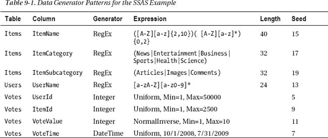
Notice that each item has a different Seed value. That helps to prevent unintended correlations between the data that can otherwise happen as a side effect of the random number generator.
Generate 2,500 rows for the Items table, 50,000 rows for Users, and 5,000,000 rows for Votes.
Data Source View
With your schema and data in place, you’re ready to start building a cube. To have the correct project type available, you should install SQL Server client tools on your machine first, either as part of installing a local instance of SQL Server or separately, but using the same installer. You can walk through the following example using either SQL Server Data Tools (SSDT), which is a special version of Visual Studio that’s installed with the SQL Server 2012 client tools, or Business Intelligent Development Studio (BIDS), which comes with SQL Server 2008:
- Right-click your solution in Solution Explorer, select Add
New Project, and then select Business Intelligence Projects in the Project types panel on the left and Analysis Services Multidimensional and Data Mining Project in the Templates panel on the right. Call the project
SampleCube, and click OK.- In the new project, right-click Data Sources in Solution Explorer and select New Data Source to start the Data Source Wizard. Click Next. In the Select how to define the connection dialog box, configure a connection to the relational database that has the schema and data you created in the previous section.
- Click Next again. In the Impersonation Information dialog box, select Use the Service Account. SSAS needs to connect directly to the relational store in order to access the relational data. This tells SSAS to use the account under which the SSAS service is running to make that connection. This should work if you kept all the defaults during the installation process. If you’ve changed any of the security settings, you may need to assign a SQL Server Auth account or add access for the SSAS service account.
- Click Next. In the Completing the Wizard dialog box, keep the default name, and click Finish to complete the creation of the data source.
- Right-click Data Source Views, and select New Data Source View to bring up the Data Source View Wizard. Click Next, and select the data source you just created.
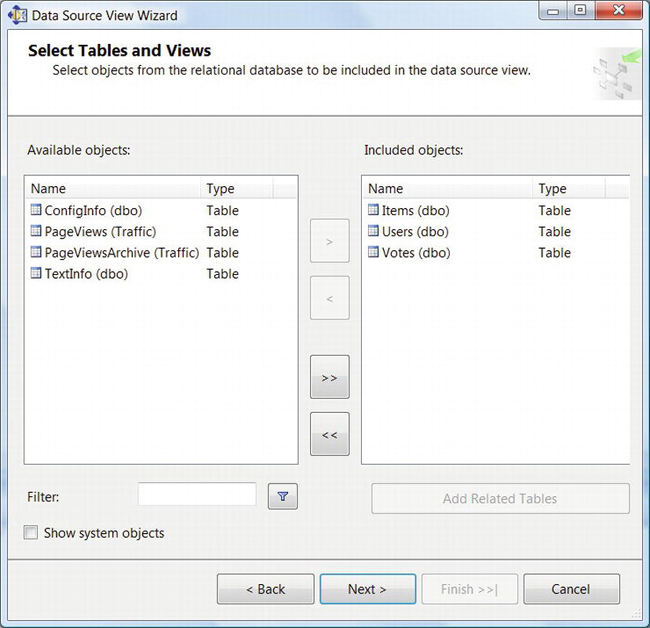
- Click Next again. In the Select Tables and Views dialog box, for each of the three tables from your test schema, click the table name in the left panel, and then click the right-arrow button to move the table name into the right panel, as shown in Figure 9-1.
- Click Next to advance to the Completing the Wizard dialog box, accept the default name, and click Finish. Doing so displays the initial DSV, as in Figure 9-2.
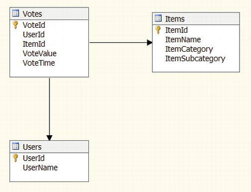
Figure 9-2. Initial data source view
You can see that the DSV shows primary keys with a small key icon. The arrows between the tables show how they’re related.
When you build the cube, you want to be able to do analysis based on the date when users placed their votes. For that to work, you need to generate a different version of the VoteTime column that contains a pure date, rather than the mixed date and time created for you by the data generator. That way, the pure date can become a foreign key in a special table (dimension) you'll create a little later.
You can do this by adding a named calculation to the Votes table. Right-click the header of the Votes table, and select New Named Calculation. Call the column VoteDate, and enter CONVERT(DATETIME, CONVERT(DATE, [VoteTime])) for the expression, as shown in Figure 9-3. That converts the combined date and time to a DATE type and then back to a DATETIME type.

Figure 9-3. Create a named calculation.
Let’s double-check that the named calculation is working correctly. Right-click the Votes table and select Explore Data. Your results should look something like Figure 9-4, particularly in the sense that the times on the VoteDate column are all zero.
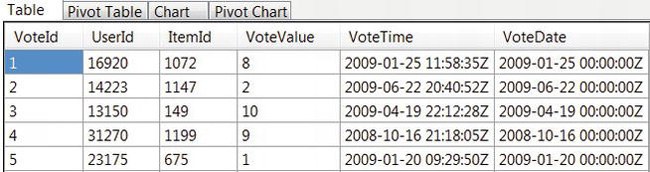
Figure 9-4. Using Explore Data to double-check the VoteDate named calculation
Cube
To create the cube, follow these steps:
- Right-click Cubes in Solution Explorer, and select New Cube to open the Cube Wizard.
- Click Next. In the Select Creation Method dialog box, accept the default of Use existing tables, because you want to create a cube based on the tables in your data source.
- Click Next. In the Select Measure Group Tables dialog box, select the
Votestable. That is your fact table, which forms the core of your measure group. Measure groups can contain more than one fact table.- Click Next. In the Select Measures dialog box, keep the default selections, with both Vote Value and Votes Count selected. Measures are numeric quantities (usually aggregations) that are associated with a fact table, such as counts and sums.
- Click Next. In the Select Dimensions dialog box, keep the default selections, which include both the
UsersandItemstables. Dimensions contain primary keys and usually one or more strings that are associated with those keys (such asUserName).- Click Next. In the Completing the Wizard dialog box, keep the default name, and click Finish. When it completes, you should see a diagram that looks very similar to the DSV in Figure 9-2, except the fact table now has a yellow title and the dimensions have blue titles.
Although it’s possible to build and deploy the cube at this point, before you can make any useful queries against it, you must add a time dimension and add the string columns from the Items and Users tables to the list of fields that are part of those dimensions.
Time Dimension
The time dimension will hold the primary keys for the VoteDate calculated member column you added to the DSV, which will be the foreign key.
To add the time dimension, follow these steps:
- Right-click Dimension in Solution Explorer, and select Add New Dimension to open the Dimension Wizard.
- Click Next. In the Select Creation Method dialog box, select Generate a time table on the server. Unlike the other two dimensions, this one will exist in SSAS only; it won’t be derived from a relational table.
- Click Next. In the Define Time Periods dialog box, set the earliest date for your data as the First Calendar Day and the end of 2009 for the Last Calendar Day. In the Time Periods section, select Year, Half Year, Quarter, Month, Week, and Date, as in Figure 9-5. Those are the periods that SSAS will aggregate for you and that you can easily query against.

- Click Next. In the Select Calendars dialog box, keep the default selection of Regular calendar.
- Click Next. In the Completing the Wizard dialog box, keep the default name, and click Finish. You should see the Dimension designer for the new wizard, which you can close.
- After creating the dimension table, you need to associate it with a column in the
Votesfact table. To do that, open the cube designer, select the Dimension Usage tab, right-click the background of the panel, and select Add Cube Dimension. In the dialog box that comes up, select the Time dimension, and click OK. Doing so adds a Time dimension row to the list of dimensions on the left of the Dimension Usage panel.- Click the box at the intersection of the Time row and the Votes column, and then click the button on the right side of that box to bring up the Define Relationship dialog box. Select a Regular relationship type, set the Granularity attribute to Date, and set the Measure Group Column to
VoteDate, as in Figure 9-6. That’s your new date-only calculated column with the time details removed so that you can use it as a foreign key into to the Time dimension.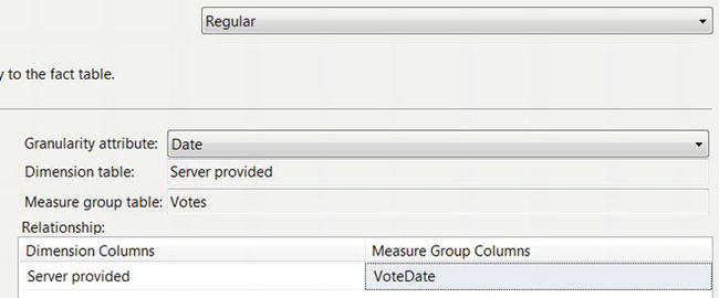
Figure 9-6. Define the relationship between the
Timedimension and theVoteDatecolumn.- Click OK. The Dimension Usage panel shows the new relationship, as in Figure 9-7.
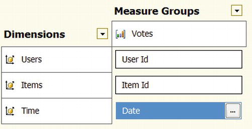
Figure 9-7. The Dimension Usage panel after adding the
Timedimension
Items and Users Dimensions
Although the cube-creation wizard added dimensions for the Items and Users tables, they only contain an ID field. To be useful for queries, you need to add the string columns as dimension attributes. For the Items dimension, you also define a hierarchy that shows how ItemSubcategory is related to ItemCategory:
- Double-click Items.dim in Solution Explorer to open the dimension designer. Click
ItemNamein the Data Source View panel on the right, and drag it to the Attributes panel on the left. Repeat forItemCategoryandItemSubcategory.- To create the hierarchy, click
Item Categoryin theAttributespanel, and drag it to the Hierarchies panel in the middle. Doing so creates a Hierarchy box in the middle panel. Then, clickItem Subcategoryin theAttributespanel, and drag it to the <new level> row in the Hierarchy box. Finally, right-click the word Hierarchy at the top of the box in the middle, select Rename, and change the name toCategories. The result should look similar to Figure 9-8.
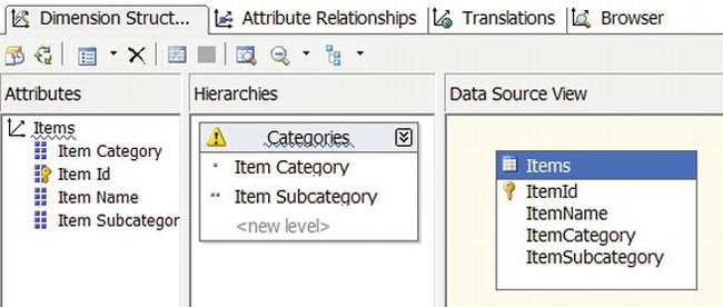
Figure 9-8. Dimension designer for the Items dimension
The warning triangle at upper left in the hierarchy definition and the blue wavy lines are there to remind you that you haven’t established a relationship between the levels. This type of a relationship could be a self-join in the original table, such as for parent-child relationships.
Notice the single dot to the left of Item Category and the two dots to the left of Item Subcategory. These are reminders of the amount of detail that each level represents. Fewer dots mean a higher level in the hierarchy and therefore less detail.
Repeat the process for the Users dimension by dragging the UserName column from the Data Source View to the Attributes panel.
Calculated Member
When determining the most popular Items on your site, one of the things you’re interested in is the average vote. You can calculate that by taking the sum of the VoteValues for the period or other slice you’re interested in and dividing by the number of votes.
To define the calculation, open the cube designer by double-clicking Sample.cube. Select the Calculations tab at the top of the designer, and click the New Calculated Member icon button (hover over a button to see a tooltip with the button’s name). Set the name of the calculation to [Vote Ave], and set the expression to the following:
[Measures].[Vote Value] / [Measures].[Votes Count]
Regardless of whether you query by date or by ItemCategory or any other dimension attribute, SSAS uses the corresponding sum and count for just the data you request.
Next, set the Format string to "0.000" to indicate that the average should include three digits to the right of the decimal place, as in Figure 9-9.
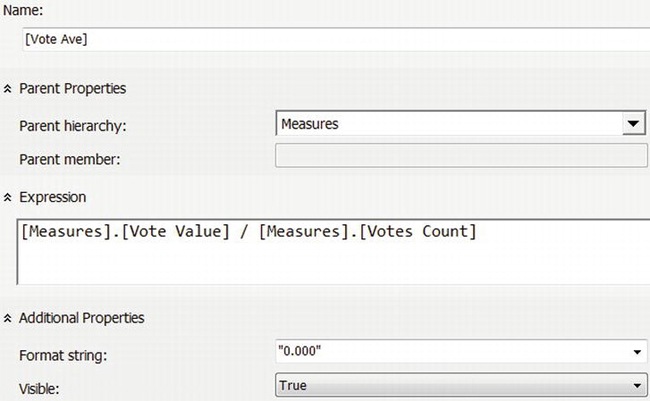
Figure 9-9. Define a calculated member for determining the average vote.
Deploy and Test
Now, you’re ready to deploy the cube to the server and to do some initial testing:
- Right-click SampleCube in Solution Explorer, and select Deploy. Doing so sends the cube definition to SSAS and tells it to use the DSV to read the data it needs from the relational database and to process the cube.
- Back in the cube designer, click the Browse tab. You will see a list of measures and dimensions on the left and a reporting panel on the right. Notice the areas that say Drop Column Fields Here, Drop Row Fields Here, and Drop Totals or Detail Fields Here.
- Expand the Votes measure in the left panel, and drag Vote Count into the center Detail Fields area. Doing so shows the total number of rows in the
Votestable, which is 5 million. Repeat the process with the Vote Ave calculated member to see the average value of all votes. Notice that Vote Ave has three digits to the right of the decimal point, as you specified in the Format String.- Expand the Items dimension, and drag Item Category to the Row Fields area. Notice how the counts and averages expand to show details based on the row values. Repeat the process for Item Subcategory, drop it to the right of the Category column, and expand the Business category to see its subcategories.
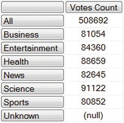
- Expand the Time dimension, and drag Half Year to the Column Fields area. The final results are shown in Figure 9-10.
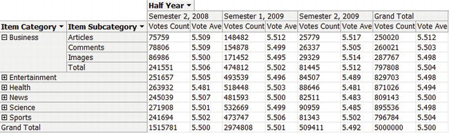
Figure 9-10. Results of testing the example cube using the Browser in SSAS
Notice how the calculations for the intermediate aggregates of date and subcategory are all calculated automatically without any additional coding.
Example MDX Queries
Here’s a T-SQL query for determining the total number of rows in the Votes table in the relational database:
SELECT

    COUNT(*) [Votes Count]

    FROM [Votes]
The result is
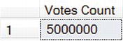
After running CHECKPOINT and DBCC DROPCLEANBUFFERS on my desktop machine, this takes about 18 seconds to run and has about 20,000 disk reads.
To use the cube from your web site, you query it using MDX. Use SSMS to test your queries.
After connecting to the relational database as you did before, click Connect in Object Explorer, select Analysis Services, provide the appropriate credentials, and click the Connect button. After it connects, expand the Databases menu, right-click SampleCube, and select New Query ![]() MDX.
MDX.
Now you can execute the following MDX query, which is equivalent to the earlier T-SQL query:
SELECT

    [Measures].[Votes Count] ON COLUMNS

    FROM [Sample]
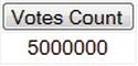
This says to use the Votes Count measure on the columns with the Sample cube. You can’t use SSMS to get time information from SSAS as you can with the relational database, but you can use SQL Profiler. It shows that the query takes about 2ms, compared to 18 seconds for the relational query.
Next, let’s look at the number of votes for the month of January 2009, grouped by ItemCategory. Here’s the T-SQL query and its result:
SELECT i.ItemCategory, COUNT(*) [Votes Count]

    FROM [Votes] v

    INNER JOIN [Items] i ON i.ItemId = v.ItemId

    WHERE v.VoteTime BETWEEN '20090101' AND '20090201'

    GROUP BY ROLLUP(i.ItemCategory)

    ORDER BY i.ItemCategory
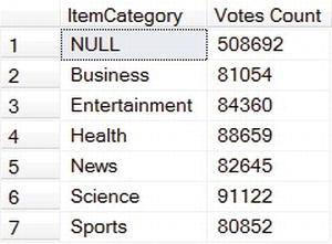
With an empty cache, this takes about 6.8 seconds to execute, still with about 20,000 disk reads. However, recall from the previous chapter that columns used to select a group of rows are good candidates for indexes. The estimated query plan tells you that you’re missing an index, so let’s create it:
CREATE NONCLUSTERED INDEX [VotesTimeIX]

    ON [Votes] ([VoteTime])

    INCLUDE ([ItemId])
Repeating the query with an empty cache shows that the execution time is now only 0.7 seconds, with about 1,400 disk reads. Let’s see how SSAS compares.
Here’s the equivalent MDX query and its result:
SELECT

        [Measures].[Votes Count] ON COLUMNS,

        [Items].[Item Category].Members ON ROWS

        FROM [Sample]

        WHERE [Time].[Month].[January 2009]
You are specifying Votes Count for the columns again, but this time the Members of the Item Category dimension are the rows. The Members include the children, such as Business, Entertainment, and so on, along with the special All member, which refers to the total.
You use the WHERE clause to specify a filter for the data that appear in the middle of the result table. In this case, you want the data for January 2009. The result is the intersection of ROWS, COLUMNS, and the WHERE clause: Votes Counts for Item Categories in January 2009.
SQL Profiler tells you that this query takes 3ms or 4ms to execute, which is well below the 700ms for its relational equivalent. This also avoids the 1,400 disk reads on the relational side and the associated reduction in memory available for other queries.
Next, let’s filter those results to show the Health row only. Here’s the relational query and its result:
SELECT

    COUNT(*) Health

    FROM [Votes] v

    INNER JOIN [Items] i ON i.ItemId = v.ItemId

    WHERE v.VoteTime BETWEEN '20090101' AND '20090201'

    AND i.ItemCategory = 'Health'
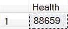
You just check for the Health category in the WHERE clause.
Here’s the MDX equivalent and its result:
SELECT

    [Measures].[Votes Count] ON COLUMNS,

    [Items].[Item Category].&[Health] ON ROWS

    FROM [Sample]

    WHERE [Time].[Month].[January 2009]
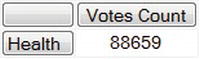
Instead of including all the Item Category members on the rows, you include only the Health row by specifying its name, preceded by an ampersand. The WHERE clause is unchanged.
Rather than getting too distracted with T-SQL, let’s focus on the MDX only from now on. You can apply the same pattern from earlier to look at average vote values for each Item:
SELECT

    [Measures].[Vote Ave] ON COLUMNS,

    [Items].[Item Name].Children ON ROWS

    FROM [Sample]

    WHERE [Time].[Month].[January 2009]
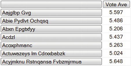
Vote Ave is the calculated member you defined earlier. For this query, you’re using Children instead of Members, which excludes the total from the All member. This query returns one row for each of the 2,500 Items. Let’s filter the results to return only the Items with the top five highest average vote values:
SELECT

    [Measures].[Vote Ave] ON COLUMNS,

    TOPCOUNT(

        [Items].[Item Name].Children,

        5,

        [Measures].[Vote Avg]

        ) ON ROWS

    FROM [Sample]

    WHERE [Time].[Month].[January 2009]
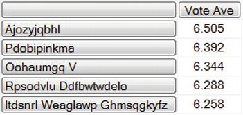
You use the TOPCOUNT() function to select the top five.
So far, your query results have had only a single column. Let’s look at the number of votes by Item Category, split out by Quarter:
SELECT

    [Time].[Quarter].Children ON COLUMNS,

    [Items].[Item Category].Children ON ROWS

    FROM [Sample]

    WHERE [Measures].[Votes Count]
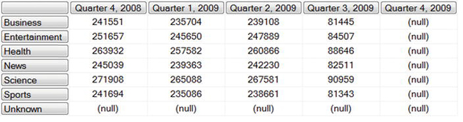
To do that, you specify the Children of the Quarter dimension as the columns. However, that result includes some null rows and columns, because you don’t have any Unknown items (Unknown is another default Member) and because you don’t have any Votes in Quarter 4, 2009.
Let’s filter out the null rows and columns:
SELECT

    NONEMPTY([Time].[Quarter].Children,

        [Items].[Item Category].Children) ON COLUMNS,

    NONEMPTY([Items].[Item Category].Children,

        [Time].[Quarter].Children) ON ROWS

    FROM [Sample]

    WHERE [Measures].[Votes Count]
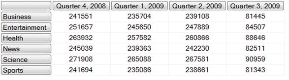
The NONEMPTY() function selects non-null entries with respect to its second argument and the WHERE clause. For example, the first call says to return only Children of the Quarter dimension that have a non-null Votes Count for all of the Item Category Children.
Let’s show just the results for the Health Category and include a breakdown by Subcategory:
SELECT

    NONEMPTY([Time].[Quarter].Children,

        [Items].[Item Category].Children) ON COLUMNS,

    ([Items].[Item Category].&[Health],

            [Items].[Item Subcategory].Children) ON ROWS

    FROM [Sample]

    WHERE [Measures].[Votes Count]
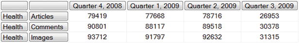
Including the Health Category and the Subcategory Children together inside parentheses is an MDX syntax that indicates they are a tuple. That’s how you specify that you want to show the Subcategories of the Health Category. In the results, notice that each row has two labels, one for each member of the tuple.
Next, let’s say that you want to see the Votes Count totals for the Health Category for the three days ending on March 7, 2009:
SELECT

    LASTPERIODS(

        3,

        [Time].[Date].[Saturday, March 07 2009]

        ) ON COLUMNS,

    [Items].[Item Category].&[Health] ON ROWS

    FROM [Sample]

    WHERE [Measures].[Votes Count]

The LASTPERIODS() function uses the position of the specified date in its dimension and includes the requested number of periods by using sibling nodes in the dimension. If you replaced the date in the query with a Quarter, the query results would show three quarters instead of three days.
Next, let’s take the sum of those three days:
WITH

    MEMBER [Measures].[Last3Days]

            AS 'SUM(LASTPERIODS(3, [Time].[Date].[Saturday, March 07 2009]),

                    [Measures].[Votes Count])'

        SELECT

                [Measures].[Last3Days] ON COLUMNS,

                [Items].[Item Category].&[Health] ON ROWS

                FROM [Sample]
![]()
You don’t have a dimension for those three days together, like you do for full weeks, months, quarters, and so on, so you have to calculate the result using the SUM() function. You use the WITH MEMBER clause to define a temporary calculated member, which you then use in the associated SELECT statement. The arguments to the SUM() function are the date range and the measure that you want to sum over those dates.
Next, let’s extend that query further by including a sum of the Vote Values for those three days, as well as the average Vote Value. Let’s also look at those values for the top five Items, based on their average vote value:
WITH

    MEMBER [Measures].[Last3DaysCount]

        AS 'SUM(LASTPERIODS(3, [Time].[Date].[Saturday, March 07 2009]),

            ([Measures].[Votes Count]))'

    MEMBER [Measures].[Last3DaysSum]

        AS 'SUM(LASTPERIODS(3, [Time].[Date].[Saturday, March 07 2009]),

            ([Measures].[Vote Value]))'

    MEMBER [Measures].[Last3DaysAvg]

        AS '[Measures].[Last3DaysSum] / [Measures].[Last3DaysCount]',

            FORMAT_STRING = '0.000'

SELECT

    {[Measures].[Last3DaysCount],

        [Measures].[Last3DaysSum],

        [Measures].[Last3DaysAvg]
        } ON COLUMNS,

    TOPCOUNT(

        [Items].[Item Name].Children,

        5,

        [Measures].[Last3DaysAvg]) ON ROWS

    FROM [Sample]
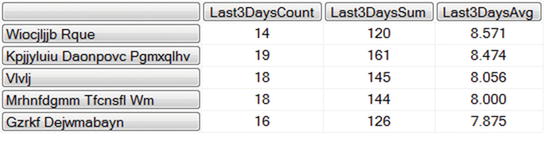
To include the three different calculated members in the columns, you specify them as a set using curly braces. Notice too that you specify a format string for Last3DaysAvg, as you did for Vote Ave when you were building the cube.
MDX is a powerful language that’s capable of much more than I’ve outlined here. Even so, the syntax and capabilities covered in this section should be enough for you to offload a number of aggregation queries from your relational database, including sums, counts, averages, topcount, lastperiods, and summaries by multiple dates or periods.
ADOMD.NET
Before you can query SSAS from your web application, you need to download and install the ADOMD.NET library, because it’s not included with the standard .NET distribution. It’s part of the Microsoft SQL Server Feature Pack (a free download).
After completing the installation, right-click your web site in Solution Explorer, and select Add Reference. On the .NET tab of the dialog box, select the latest version of Microsoft.AnalysisServices.AdomdClient, and click OK. See Figure 9-11.
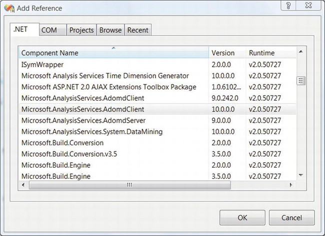
Figure 9-11. Add a reference to the ADOMD.NET library.
Example with a Single-Cell Result
For the first example, let’s make a web page that displays a single result from an MDX query. In particular, the query retrieves the total number of votes for the Health Category for January 2009.
First, create a new web form called mdx1.aspx, and edit the markup as follows:
<%@ Page Language="C#" EnableViewState="false" AutoEventWireup="false"

    CodeFile="mdx1.aspx.cs" Inherits="mdx1" %>

<!DOCTYPE html PUBLIC "-//W3C//DTD XHTML 1.0 Transitional//EN"

    "http://www.w3.org/TR/xhtml1/DTD/xhtml1-transitional.dtd">

<html xmlns="http://www.w3.org/1999/xhtml">

<body>

Total

<asp:Label ID="RowName" runat="server" />

votes for January 2009:

<asp:Label ID="TotHealthVotes" runat="server" />

</body>

</html>
The markup mainly has two <asp:Label> controls, which you use to display the results.
Here’s the code-behind:
using System;

using System.Web.UI;

using Microsoft.AnalysisServices.AdomdClient;


public partial class mdx1 : Page

{

    private const string connStr = "data source=.;initial catalog=SampleCube";


    protected override void OnLoad(EventArgs e)

    {

        base.OnLoad(e);

        using (AdomdConnection conn = new AdomdConnection(connStr))

        {

            const string mdx = "SELECT " +

                    "[Measures].[Votes Count] ON COLUMNS, " +

                    "[Items].[Item Category].&[Health] ON ROWS " +

                    "FROM [Sample] " +

                    "WHERE [Time].[Month].[January 2009]";

            using (AdomdCommand cmd = new AdomdCommand(mdx, conn))

            {

                conn.Open();

                var reader = cmd.ExecuteReader();

                if (reader.Read())

                {

                    this.RowName.Text = reader[0].ToString();

                    this.TotHealthVotes.Text = reader[1].ToString();

                }

            }

        }

    }

}
You can see that the code pattern for using ADOMD.NET is analogous to standard ADO.NET. You are mainly just replacing SqlConnection with AdomdConnection, and SqlCommand with AdomdCommand. The library doesn’t have a native asynchronous interface like ADO.NET, so you’re using a synchronous page.
One difference compared with the relational database is that you have to include the full text of the MDX query, because SSAS doesn’t support stored procedures in the same way. The result set is also somewhat different, because each row can have labels, in addition to each column. The difference isn’t too noticeable here, because the result has only one row, with a label in column 0 and the result in column 1. It is more apparent in the next example.
When you run the page, it displays the following:
Total Health votes for January 2009: 88659
You can use a query like this to avoid executing the equivalent aggregation query on the relational side. In a production system, you may want to cache the result at your web tier to avoid executing the query more often than necessary.
Displaying a Multiple-Row Result Using a GridView
For the next example, let’s display the results of an MDX query that returns a number of rows. Let’s look at the number of votes for each Category for January 2009.
Here’s the markup for mdx2.aspx:
<%@ Page Language="C#" EnableViewState="false" AutoEventWireup="false"

    CodeFile="mdx2.aspx.cs" Inherits="mdx2" %>

<!DOCTYPE html PUBLIC "-//W3C//DTD XHTML 1.0 Transitional//EN"

    "http://www.w3.org/TR/xhtml1/DTD/xhtml1-transitional.dtd">

<html xmlns="http://www.w3.org/1999/xhtml">

<head runat="server">

    <title></title>

</head>

<body>

    <form id="form1" runat="server">

    <div>

        <asp:GridView ID="MdxGrid" runat="server" />

    </div>

    </form>

</body>

</html>
You have an <asp:GridView> control that holds the results.
Here’s the code-behind:
using System;

using System.Data;

using System.Web.UI;

using Microsoft.AnalysisServices.AdomdClient;


public partial class mdx2 : Page

{

    private const string connStr = "data source=.;initial catalog=SampleCube";


    protected override void OnLoad(EventArgs e)

    {

        base.OnLoad(e);

        using (AdomdConnection conn = new AdomdConnection(connStr))

        {

            const string mdx = "SELECT " +

                               "[Measures].[Votes Count] ON COLUMNS, " +

                               "[Items].[Item Category].Members ON ROWS " +

                               "FROM [Sample] " +

                               "WHERE [Time].[Month].[January 2009]";

            using (AdomdCommand cmd = new AdomdCommand(mdx, conn))

            {

                conn.Open();

                CellSet cs = cmd.ExecuteCellSet();

                DataTable dt = new DataTable();

                dt.Columns.Add(" ");

                Axis columns = cs.Axes[0];

                TupleCollection columnTuples = columns.Set.Tuples;
                for (int i = 0; i < columnTuples.Count; i++)

                {

                    dt.Columns.Add(columnTuples[i].Members[0].Caption);

                }

                Axis rows = cs.Axes[1];

                TupleCollection rowTuples = rows.Set.Tuples;

                int rowNum = 0;

                foreach (Position rowPos in rows.Positions)

                {

                    DataRow dtRow = dt.NewRow();

                    int colNum = 0;

                    dtRow[colNum++] = rowTuples[rowNum].Members[0].Caption;

                    foreach (Position colPos in columns.Positions)

                    {

                        dtRow[colNum++] =

                            cs.Cells[colPos.Ordinal, rowPos.Ordinal].FormattedValue;

                    }

                    dt.Rows.Add(dtRow);

                    rowNum++;

                }

                this.MdxGrid.DataSource = dt;

                this.MdxGrid.DataBind();

            }

        }

    }

}
The outer structure of the code is the same as the first example, with AdomdConnection and AdomdCommand. However, this time you’re using ExecuteCellSet() to run the query. It returns a CellSet object, which is the multidimensional equivalent of a DataTable. Unfortunately, you can’t bind a CellSet directly to the GridView control, so you have to do some work to transform it into a DataTable, which you can then bind to the grid.
See Figure 9-12 for the results.
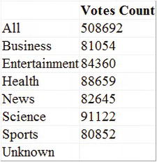
Figure 9-12. Web page containing a multirow MDX query result
Updating Your Cube with SSIS
As you’ve been developing your example cube, you've only been pulling over new data from the relational engine when you manually reprocess the cube. SSAS retrieves data from the relational engine through the DSV you created along with the cube.
In a production environment, you would, of course, want to automate that process. One approach is to use SQL Server Integration Services (SSIS) to run a task that tells SSAS to process the cube in the same way as previously. You can then create a job in SQL Agent to run that task once a day or as often as you need it.
Let’s walk through the process:
- Right-click your solution in Solution Explorer, and select Add
SampleSSIS, and click OK.- Right-click
SampleSSIS, and select AddProcessCube.dtsx, and click Add. Doing so opens the SSIS package designer with the Control Flow tab selected by default.- Click the Toolbox panel, and drag Analysis Services Processing Task from the Toolbox to the surface of the SSIS package designer. See Figure 9-13.
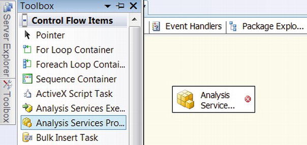
Figure 9-13. Adding the Analysis Services Processing task to the SSIS package
- Double-click the task to open its task editor. Select Processing Settings in the left panel, and click New in the right panel to add a new connection manager. In the Add Analysis Services Connection Manager dialog box, click Edit. In the Connection Manager dialog box, define your connection parameters, and set the Initial Catalog to
SampleCube. Click Test Connection, and then click OK. See Figure 9-14.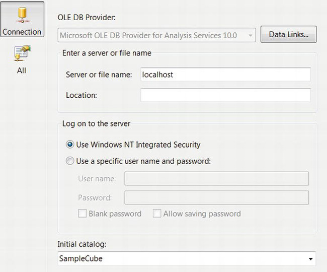
Figure 9-14. Adding a connection manager for the example cube
- Click OK again to get back to the Analysis Services Processing Task Editor. To specify the cube that you want to process, click Add, select SampleCube, and click OK. See Figure 9-15. Notice that, by default, Process Options is set to Process Full, which tells SSAS to re-create the data in the cube from scratch using the DSV you configured earlier. Click OK again to dismiss the editor.
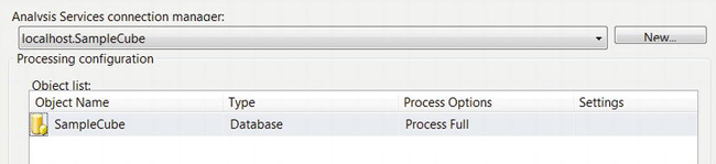
Figure 9-15. Configure the cube in the Analysis Services Processing Task Editor.
- At this point, you can test the package in debug mode. Right-click
ProcessCube.dtsxin Solution Explorer, and select Execute Package. You should see the task box turn yellow while it’s running and then turn green when it completes.- To complete the process of automating the task, copy the
ProcessCube.dtsxfile to your server. Open SSMS, connect to your relational database, right-click SQL Server Agent in Object Explorer, and select NewProcess Cube, and click Steps on the left panel, where you define what this job does. Click New, and call the step Run SSIS Processing Task. For the job Type, select SQL Server Integration Services Package. For Package source, select File system, and set the path to theProcessCube.dtsxfile. See Figure 9-16. Click OK.
Figure 9-16. Configure a SQL Server Agent job step with an SSIS Processing Task.
- Select Schedules in the left panel, and configure how often you want the task to run. If once-per-day processing is enough, choose a time of day when your site isn’t busy, in order to reduce the impact on your live site. Click OK to finish configuring the job.
After configuring the job, you can test it by right-clicking the job name in Object Explorer and selecting Start job at step.
The approaches to cube processing discussed so far have involved SSAS pulling data from the relational store. It is also possible to push data into SSAS using a different type of SSIS task. Pushing data is useful in cases where you also need to manipulate or transform your data in some way before importing it into a cube, although a staging database is preferable from a performance perspective (see the section on staging databases later in this chapter).
Proactive Caching
A much more efficient way to automate cube updates in your production environment is with a SQL Server Enterprise, Business Intelligence and Developer edition-only feature called proactive caching.
Data Storage Options
SSAS maintains two different types of data. One is measure group data, which includes your fact and dimension tables, also known as leaf data. The other is precalculated aggregations. You can configure SSAS to store each type of data either in a native SSAS-specific format or in the relational database. You have three options:
- Multidimensional OLAP, or MOLAP mode, stores both the measure group data and the aggregation data in SSAS. Aggregates and leaf data are stored in a set of files in the local filesystem. SSAS runs queries against those local files.
- Relational OLAP, or ROLAP mode, stores both the measure group data and the aggregation data in the relational database.
- Hybrid OLAP, or HOLAP mode, stores aggregations in local files and stores the leaf data in the relational database.
MOLAP mode generally provides the best query performance. However, it requires an import phase, which can be time-consuming with large datasets. ROLAP is generally the slowest. You can think of both ROLAP and HOLAP as being “real time” in the sense that OLAP queries reflect the current state of the relational data. Because these modes make direct use of your relational database during query processing, they also have an adverse effect on the performance of your database, effectively defeating one of your main motivations for using SSAS in the first place.
You can configure the storage mode from the Partitions tab in the cube designer. Right-click the default partition, and select Storage Settings. See Figure 9-17.
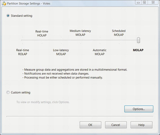
Figure 9-17. Partition storage settings
Caching Modes
SSAS supports several different processing-related settings for proactive caching. Click the Options button in the dialog box in Figure 9-17. See Figure 9-18.
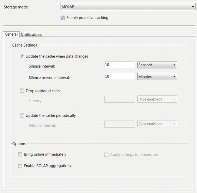
Figure 9-18. Proactive caching options
Select the Enable proactive caching check box to enable the options.
One option is to process the cube, also known as updating the cache, when SSAS receives a notification from the relational database that the data has changed. There are two parameters: the silence interval is how long SSAS should try to wait after the last change notification before processing the cube. Silence override interval is how long SSAS waits after receiving the first change notification, but without the silence interval being satisfied. The net effect is that if there is a short burst of activity on the staging database, SSAS processes the cube after the silence interval. If the activity goes on for a long time, then it delays processing until the silence override interval has passed.
The next option is whether SSAS should Drop outdated cache (the imported and processed data). The Latency parameter is the time beginning when it starts rebuilding the cube and ending when it drops the cache.
You can also configure SSAS to Update the cache periodically—for example, once per day. That mode does not depend on SSAS receiving change notifications from the relational engine. The other modes require Service Broker to be enabled so that change notifications work.
If you select Bring online immediately, then SSAS sends ROLAP queries to the relational database while the cube is being rebuilt. You must select this option if Drop outdated cache is selected. With both options selected, the effect is that when a change is detected, the MOLAP cache is dropped after the latency period. Subsequent OLAP queries are then redirected to the relational database using ROLAP. When the cube processing has completed, queries are again processed using MOLAP.
The Enable ROLAP aggregations option causes SSAS to use materialized views in the relational database to store aggregations. This can improve the performance of subsequent queries that use those aggregates when the cube is using ROLAP mode.
Together, you can use these settings to manage both the cube refresh interval and the perceived latency against the staging database. The main trade-off when using Bring online immediately is that, although it has the potential to reduce latency after new data has arrived in the staging database, ROLAP queries may be considerably slower than their MOLAP counterparts because aggregations must be computed on the fly. The resulting extra load on the relational database also has the potential of slowing down both the cube-rebuilding process and your production OLTP system. Therefore, although it’s appealing on the surface, you should use this option with care, especially for large cubes.
To configure relational database notifications, click the Notifications tab, and select SQL Server and Specify tracking tables. Click the button to the right, select the Items, Users, and Votes tables, and click OK. See Figure 9-19.
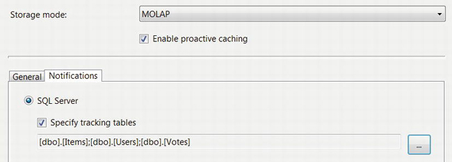
Figure 9-19. Specify SQL Server notifications for proactive caching.
![]() Note Only tables are allowed for SQL Server notifications. The use of views or stored procedures is not supported.
Note Only tables are allowed for SQL Server notifications. The use of views or stored procedures is not supported.
After making the configuration changes, deploy the cube to the server so that the changes take effect.
You can test your proactive caching settings as follows. First, issue the following MDX query from SSMS, which shows the number of rows in the fact table:
Next, make a change to the relational data by inserting a row into the Votes table:
INSERT INTO Votes

    (UserId, ItemId, VoteValue, VoteTime)

    OUTPUT INSERTED.VoteId

    VALUES

    (2, 2, 1, GETDATE())
After allowing enough time for your configured silence interval to pass, along with time to reprocess the cube, issue the MDX query again. You should see that the reported count has increased by one.
The achievable cube-refresh interval ultimately depends on factors such as the following:
- The amount of new data at each refresh
- Available hardware on both the relational database and the SSAS machines: CPU count and speed, amount of RAM, speed of disks and number of available LUNs or channels, and speed of the network between the machines
- Speed of the relational database, including both how fast it can deliver data to SSAS and how fast it can process aggregation queries in ROLAP mode
- If you’re using SSIS for data import: how fast it can pull data from the production databases (query complexity, production database machine speed, and load during the ETL process)
- Amount of preaggregation done in each partition in the cube (additional preaggregation can improve the performance of some queries but requires more time during cube processing)
- Total number of dimension attributes
- Other performance-related parameters and settings in SSAS, such as partition configurations, hierarchies, and so on
Using a Staging Database
Although allowing SSAS to import data directly from your production relational database/OLTP system can be acceptable in some scenarios, it is often better from a performance and scalability perspective to use a staging database instead.
A staging database is another relational database that sits between your OLTP store and SSAS. It differs from your OLTP store in the following ways:
- It is organized structurally with a star snowflake schema that’s similar to your cubes, with one or more central fact tables and associated dimension tables.
- It contains more historical data, leaving only reasonably current data on your OLTP system.
- You should configure the hardware to support bulk I/O, optimized for queries that return many more rows on average than your OLTP system.
This type of system is sometimes also called a data warehouse, although I prefer to use that term to refer to a collection of data marts, where each data mart contains an OLTP system, a staging database, and SSAS.
A staging database has the following benefits:
- You can run queries against the staging database without affecting the performance of your OLTP system.
- SSAS can import data from the staging database so the process doesn’t burden your production OLTP system (although you still need to import data into the staging database).
- You can offload (partition) your OLTP database by moving older archival data into the staging database and keeping transaction tables relatively short.
- The staging database provides a solid base that you can use to rebuild cubes from scratch if needed, without adversely affecting the performance of your OLTP system.
A typical architecture involves using SSIS to create a database snapshot on your OLTP system and then pulling data from the snapshot (which helps keep it consistent), transforming the data, and storing the data in the staging database. SSAS then uses proactive caching to receive notifications when the staging database changes, and pulls data from there for processing your cubes. See Figure 9-20.
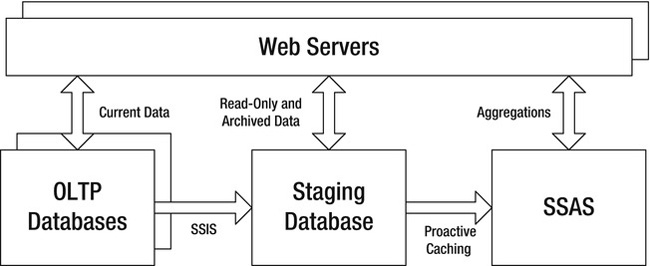
Figure 9-20. Data tier architecture with a staging database and SSAS
You can run production queries against all three data stores: the OLTP system for current data, the staging database for read-only and archived data, and SSAS for aggregation queries. You can run back-end reports from either the staging database or SSAS, or both.
During the ETL process, SSIS can perform functions such as the following:
- Data cleansing
- Ensuring fact table foreign keys are present as primary keys in the corresponding dimensions
- Removing unused columns
- Data denormalization (joins across multiple tables)
- Creating new columns that are derived from existing columns
- Replacing production keys with surrogate keys (optional, but recommended)
- Split tables into facts and dimensions (which should result in much smaller dimensions)
- Handling incremental updates so the entire staging database doesn’t need to be rebuilt each time
While designing the SSIS packages to move data from your OLTP system to a staging database, you should also analyze each dimension and fact table:
- Which columns should be included? You should only include columns needed in the cube.
- Can rows in the table ever change? If so, a slowly changing dimension (SCD) will probably be required.
- How should changes be managed? Updated or historical?
- Are there any data transformations that should be done during the export, transform, and load (ETL) process, such as converting
DATETIMEvalues to date-only as in the example?- Review the business keys on the relational side to make sure new ones are always increasing and to verify that there aren’t any unexpected values (negative numbers, nulls, and so on).
- For fact tables that are also dimensions, fact columns should be extracted and placed into a separate table from the dimension columns.
- Look for optimizations that may be possible for the resulting dimension tables, such as removing duplicates.
As the amount of data that you are processing increases, there may eventually be a time when the structure of some queries should change for performance reasons. For example, if a multitable join for the fact tables gets too slow or puts too much of a load on the source database, you can replace it with a sequence of Lookup steps in the data flow.
Summary
In this chapter, I covered the following:
- Using SSAS to offload aggregation queries from your relational database and why that’s important from a performance and scalability perspective
- Understanding SSAS and multidimensional databases
- Building an example cube
- Using example MDX queries against the sample cube
- Using ADOMD.NET to programmatically send MDX queries to SSAS and display the results on a web page
- Using SSIS and SQL Server Agent to update your cube
- Using proactive caching to reduce the latency between changes in your relational data and corresponding updates to your cubes
- Using a staging database to reduce the load on your OLTP server during cube processing