C H A P T E R  8

SQL Server Relational Database

In this chapter, I’ll cover a few areas that can have a large impact on the performance of your data tier, even if you have already optimized your queries fully.

For example, our principle of minimizing round-trips also applies to round-trips between the web tier and the database. You can do that using change notifications, multiple result sets, and command batching.

The topics that I’ll cover include the following:

• How SQL Server manages memory
• Stored procedures
• Command batching
• Transactions
• Table-valued parameters
• Multiple result sets
• Data precaching
• Data access layer
• Query and schema optimization
• Data paging
• Object relational models
• XML columns
• Data partitioning
• Full-text search
• Service Broker
• Data change notifications
• Resource Governor
• Scaling up vs. scaling out
• High availability
• Miscellaneous performance tips

How SQL Server Manages Memory

Similar to ASP.NET, it’s possible to have a fast query (or page) but a slow database (or site). One of the keys to resolving this and to architecting your database for speed is to understand how SQL Server manages memory.

Memory Organization

On 32-bit systems, SQL Server divides RAM into an area that can hold only data pages and a shared area that holds everything else, such as indexes, compiled queries, results of joins and sorts, client connection state, and so on. 32 bits is enough to address up to 4GB at a time. The default configuration is that 2GB of address space is reserved for the operating system, leaving 2GB for the application. When running under one of the 32-bit versions of Windows Server, SQL Server can use Address Windowing Extensions (AWE) to map views of up to 64GB dynamically into its address space. (AWE isn’t available for the desktop versions of Windows.) However, it can use memory addressed with AWE only for the data area, not for the shared area. This means that even if you have 64GB of RAM, with a 32-bit system you might have only 1GB available for shared information.

You can increase the memory available to 32-bit versions of SQL Server on machines with 16GB or less by adding the /3GB flag in the operating system’s boot.ini file. That reduces the address space allocated to the operating system from 2GB to 1GB, leaving 3GB for user applications such as SQL Server. However, since limiting the RAM available to the OS can have an adverse effect on system performance, you should definitely test your system under load before using that switch in production.

On 64-bit systems, the division between data pages and shared information goes away. SQL Server can use all memory for any type of object. In addition, the memory usage limit increases to 2TB. For those reasons, combined with the fact that nearly all CPUs used in servers for quite a few years now are capable of supporting 64-bit operating systems (so there shouldn’t be any additional hardware or software cost), I highly recommend using 64-bit systems whenever possible.

Reads and Writes

SQL Server uses three different kinds of files to store your data. The primary data store, or MDF file, holds tables, indexes, and other database objects. You can also have zero or more secondary data stores, or NDF files, which hold the same type of content in separate filegroups. The LDF file holds the database log, which is a list of changes to the data file.

The MDF and NDF files are organized as 64KB extents, which consist of eight physically contiguous 8KB pages. Table or index rows are stored on a page serially, with a header at the beginning of the page and a list of row offsets at the end that indicate where each row starts in the page. Rows can’t span multiple pages. Large columns are moved to special “overflow” pages.

When SQL Server first reads data from disk, such as with a SELECT query, it reads pages from the data files into a pool of 8KB buffers, which it also uses as a cache. When the pool is full, the least-recently used buffers are dropped first to make room for new data.

Since SQL Server can use all available memory as a large cache, making sure your server has plenty of RAM is an important step when it comes to maximizing performance. It would be ideal if you have enough room to fit the entire database in RAM. See the “Scaling Up vs. Scaling Out” section in this chapter for some tips on how to determine whether your server needs more memory. Based on my experience, it’s common in high-performance sites to see database servers with 32GB of RAM or more.

When you modify data, such as with an INSERT, UPDATE, or DELETE, SQL Server makes the requested changes to the data pages in memory, marks the associated data buffers as modified, writes the changes to the database log file (LDF), and then returns to the caller after the log write completes. A dedicated “lazy writer” thread periodically scans the buffer pool looking for modified buffers, which it writes to the data file (MDF). Modified buffers are also written to the MDF file if they need to be dropped to make room for new data or during periodic checkpoints.

Writes to the log file are always sequential. When properly configured on a disk volume by itself, the disk heads shouldn’t have to move very much when writing to the log file, and write throughput can be very high.

Writes to the data file will generally be at random locations in the MDF file, so the disk heads will move around a lot; throughput is normally a small fraction of what’s possible with an equivalently configured log drive. In fact, I’ve seen a factor of 50-to-1 performance difference, or more, between random and sequential writes on similar drives. See Chapter 10 for details.

To avoid seeks and thereby maximize write throughput, it’s especially important to have the database log file on a set of dedicated spindles, separate from the data file.

Performance Impact

Understanding the way that SQL manages memory leads to several important conclusions:

• The first time you access data will be much slower than subsequent accesses, since data has to be read from disk into the buffer cache. This can be very important during system startup and during a database cluster failover, since those servers will start with an empty cache. It also leads to the beneficial concepts of database warm-up and precaching of database content.
• Aggregation queries (sum, count, and so on) and other queries that scan large tables or indexes can require a large number of buffers and have a very adverse effect on performance if they cause SQL Server to drop other data from the cache.
• With careful design, it’s possible to use SQL Server as an in-memory cache.
• Write performance is determined largely by how fast SQL Server can sequentially write to the log file, while read performance is mostly determined by a combination of the amount of RAM available and how fast it can do random reads from the data file.
• When writes to the database log start happening simultaneously with the lazy writer thread writing modified pages to the data file, or simultaneously with data reads hitting the disk, the resulting disk seeks can cause the speed of access to the log file to decrease dramatically if the log and data files are on the same disk volume. For that reason, it’s important to keep the log and data files on separate disk spindles.

Stored Procedures

Using stored procedures as your primary interface to the database has a number of advantages:

• Stored procedures allow easy grouping and execution of multiple T-SQL statements, which can help reduce the number of round-trips that the web server requires to perform its tasks.
• They allow you to make changes on the data tier without requiring changes on the web tier. This helps facilitate easy and fast application evolution and iterative improvement and tuning of your schema, indexes, queries, and so on.
• They more easily support a comprehensive security framework than dynamic SQL. You can configure access to your underlying tables and other objects so that your web tier can access them only through a specific set of procedures.

Another way to think of it is that stored procedures are a best practice for the same reason that accessors are a best practice in object-oriented code: they provide a layer of abstraction that allows you to modify easily all references to a certain object or set of objects.

When you submit a command to SQL Server, it needs to be compiled into a query plan before it can be executed. Those plans can be cached. The caching mechanism uses the command string as the key for the plan cache; commands that are exactly the same as one another, including whitespace and embedded arguments, are mapped to the same cached plan.

In dynamic ad hoc T-SQL, where parameters are embedded in the command, SQL Server performs an optimization that automatically identifies up to one parameter. This allows some commands to be considered the same so they can use the same query plan. However, if the command varies by more than one parameter, the extra differences are still part of the string that’s used as the key to the plan cache, so the command will be recompiled for each variation. Using stored procedures and parameterized queries can help minimize the time SQL Server spends performing compilations, while also minimizing plan cache pollution (filling the cache with many plans that are rarely reused).

When you’re writing stored procedures, one of your goals should be to minimize the number of database round-trips. It’s much better to call one stored procedure that invokes ten queries than ten separate procedures that invoke one query each. I generally don’t like to get too much business logic in them, but using things like conditionals is normally fine. Also, keep in mind that, as with subroutines or even user controls, it’s perfectly acceptable for one stored procedure to call another one.

I suggest using dynamic T-SQL only when you can’t create the queries you need with static T-SQL. For those times when it’s unavoidable, be sure to use parameterized queries for best performance and security. Forming queries by simply concatenating strings has a very good chance of introducing SQL injection attack vulnerabilities into your application.

Here’s an example of creating a table and a stored procedure to access it. I’m also using a SCHEMA, which is a security-related best practice:

The stored procedure gets the current date, inserts a row into the [Traffic].[PageViews] table, and returns the resulting primary key as an output variable.

You will be using these objects in examples later in the chapter.

Command Batching

Another way to reduce the number of database round-trips is to batch several commands together and send them all to the server at the same time.

Using SqlDataAdapter

A typical application of command batching is to INSERT many rows. As an example, let’s create a test harness that you can use to evaluate the effect of using different batch sizes. Create a new web form called sql-batch1.aspx, and edit the markup to include the following:

You will use the two text boxes to set the record count and the batch size and an <asp:Literal> to display the results.

The conventional way to do command batching for INSERTs, UPDATEs, and DELETEs with ADO.NET is to use the SqlDataAdapter class. Edit the code-behind as follows:

After parsing the input parameters and creating a SqlConnection, in a loop that’s executed once for each batch, create a new DataTable with three columns that correspond to the database table.

Next, create a SqlCommand object that references the stored procedure, and define its parameters, including their data types and the names of the columns that correspond to each one. Notice that the first parameter has its Direction property set to ParameterDirection.Output to indicate that it’s an output parameter.

Next, set UpdatedRowSource to UpdateRowSource.OutputParameters to indicate that the runtime should map the pvid output parameter of the stored procedure back into the DataTable. Set UpdateBatchSize to the size of the batch, and add rows to the DataTable with the data. Then call adapter.Update() to synchronously send the batch to the server, and get the pvid response from the last row. In the event of an exception, write an entry in the operating system Application log.

Then you display the pvid of the last record along with the connection statistics, using the <asp:Literal> control. Each time you submit the page, it will add the requested number of rows to the PageViews table.

Results

The client machine I used for the examples in this chapter had a 6-core 2.67GHz Xeon X5650 CPU with 24GB of RAM running 64-bit Windows 7 Ultimate. SQL Server 2012 RC0 Enterprise was running under 64-bit Windows Server 2008 R2 Enterprise as a virtual machine on the same physical box, configured as a single CPU with 4-cores and 4GB RAM. The database data file was on an 8-drive RAID-50 volume, and the log file was on a 2-drive RAID-0. Both volumes used MLC SSD drives.

Here are the results after adding 20,000 rows on my test server, with a batch size of 50:

The test took 400 round-trips and about 7.7 seconds to execute. In Table 8-1, I’ve shown the results of running the test for various batch sizes, while maintaining the number of rows at 20,000.

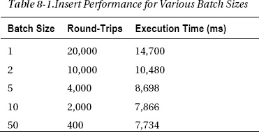
You can see that throughput roughly doubles as you increase the batch size from 1 to 10 and that larger batch sizes don’t show any additional improvement (or they might even be a little slower). At that point, you are limited by disk speed rather than round-trips.

Limitations

Although this technique works reasonably well for INSERTs, it’s not as good for UPDATEs and DELETEs, unless you already happen to have populated a DataTable for other reasons. Even then, SqlDataAdapter will send one T-SQL command for each modified row. In most real-life applications, a single statement with a WHERE clause that specifies multiple rows will be much more efficient, when possible.

This highlights a limitation of this approach, which is that it’s not general purpose. If you want to do something other than reflect changes to a single DataTable or DataSet, you can’t use the command batching that SqlDataAdapter provides.

Another issue with SqlDataAdapter.Update() is that it doesn’t have a native async interface. Recall from earlier chapters that the general-purpose async mechanisms in .NET use threads from the ASP.NET thread pool, and therefore have an adverse impact on scalability. Since large batches tend to take a long time to run, not being able to call them asynchronously from a native async interface can cause or significantly compound scalability problems, as described earlier.

Building Parameterized Command Strings

The alternative approach is to build a parameterized command string yourself, separating commands from one another with semicolons. As crude as it might sound, it’s very effective, and it addresses the problems with the standard approach in that it will allow you to send arbitrary commands in a single batch.

As an example, copy the code and markup from sql-batch1.aspx into a new web form called sql-batch2.aspx, and edit the code-behind, as follows:

Add Async=True to the connection string and to the Page directive in the .aspx file. Add the async keyword to the declaration for the Page_Load() method.

You construct the batch command by using EXEC to call your stored procedure, appending a number to the end of each parameter name to make them unique, and using a semicolon to separate each command.

To finish building the batch command, assign a value to each numbered parameter. As in the previous example, pvid is an output parameter, userid is set to a new GUID, and pvurl is a string.

Next, asynchronously execute and await all the batches you need to reach the total number of records requested and collect and display the resulting statistics.

The reported ExecutionTime statistic is much lower than with the previous example (about 265ms for a batch size of 50), which shows that ExecuteNonQueryAsync() is no longer waiting for the command to complete. However, from the perspective of total elapsed time, the performance of this approach is about the same. The advantages of this approach are that you can include arbitrary commands and that it runs asynchronously.

Transactions

As I mentioned earlier, each time SQL Server makes any changes to your data, it writes a record to the database log. Each of those writes requires a round-trip to the disk subsystem, which you should try to minimize. Each write also includes some overhead. Therefore, you can improve performance by writing multiple changes at once. The way to do that is by executing multiple writes within one transaction. If you don’t explicitly specify a transaction, SQL Server transacts each change separately.

There is a point of diminishing returns with regard to transaction size. Although larger transactions can help improve disk throughput, they can also block other threads if the commands acquire any database locks. For that reason, it’s a good idea to adopt a middle ground when it comes to transaction length – not too short and not too long – to give other threads a chance to run in between the transactions.

Copy the code and markup from sql-batch2.aspx into a new web form called sql-batch3.aspx, and edit the inner loop, as follows:

Call conn.BeginTransaction() to start a new transaction. Associate the transaction with the SqlCommand object by setting cmd.Transaction.

After the query is executed, call trans.Commit() to commit the transaction. If the query throws an exception, then call trans.Rollback() to roll back the transaction (in a production environment, you may want to wrap that call in a separate try / catch block, in case it fails).

Table 8-2 shows the results of the performance tests, after truncating the table first to make sure you’re starting from the same point.

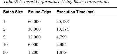
Notice that the number of round-trips has tripled in each case. That’s because ADO.NET sends the BEGIN TRANSACTION and COMMIT TRANSACTION commands in separate round-trips. That, in turn, causes the performance for the first case to be worse than without transactions, since network overhead dominates. However, as the batch size increases, network overhead becomes less significant, and the improved speed with which SQL Server can write to the log disk becomes apparent. With a batch size of 50, inserting 20,000 records takes only 24 percent as long as it did without explicit transactions.

Using Explicit BEGIN and COMMIT TRANSACTION Statements

Partly for fun and partly because the theme of this book is, after all, ultra-fast ASP.NET, you can eliminate the extra round-trips by including the transaction commands in the text of the command string. To illustrate, make a copy of sql-batch2.aspx (the version without transaction support), call it sql-batch4.aspx, and edit the part of the code-behind that builds the command string, as follows:

The T-SQL syntax allows you to use semicolons to separate all the commands except BEGIN CATCH and END CATCH. For those, you should use newlines instead.

Table 8-3 shows the test results. Notice that the difference from the previous example is greatest for the smaller batch sizes and diminishes for the larger batch sizes. Even so, the largest batch size is about 14 percent faster, although the code definitely isn’t as clean as with BeginTransaction().

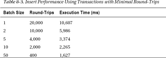
Table-Valued Parameters

T-SQL doesn’t support arrays. In the past, developers have often resorted to things like comma-separated strings or XML as workarounds. SQL Server 2008 introduced table-valued parameters. The idea is that since tables are somewhat analogous to an array, you can now pass them as arguments to stored procedures. This not only provides a cleaner way to do a type of command batching, but it also performs well, assuming that the stored procedure itself uses set-based commands and avoids cursors.

To extend the previous examples, first use SQL Server Management Studio (SSMS) to add a new TABLE TYPE and a new stored procedure.

You use the TABLE TYPE as the type of one of the arguments to the stored procedure. T-SQL requires that you mark the parameter READONLY. The body of the stored procedure uses a single insert statement to insert all the rows of the input table into the destination table. It also returns the last identity value that was generated.

To use this procedure, copy the code and markup from sql-batch1.aspx to sql-batch5.aspx, add the async keywords to the Page directive, connection string and method declaration as in the previous examples, and edit the main loop, as follows:

Here’s what the code does:

• Creates a DataTable with the two columns that you want to use for the database inserts.
• Adds batchSize rows to the DataTable for each batch, with your values for the two columns
• Configures the SqlParameters for the command, including setting pvid as an output value and adding the DataTable as the value of the rows table-valued parameter. ADO.NET automatically transforms the DataTable into a table-valued parameter.
• Asynchronously executes the command and retrieves the value of the output parameter.
• Catches database exceptions and writes a corresponding message to the Windows error log.

In addition to providing a form of command batching, this version also has the advantage of executing each batch in a separate transaction, since the single insert statement uses one transaction to do its work.

It’s worthwhile to look at the command that goes across the wire, using SQL Profiler. Here’s a single batch, with a batch size of 2:

Notice that the DataTable rows are inserted into an in-memory table variable, which is then passed to the stored procedure.

Table 8-4 shows the performance of this approach.

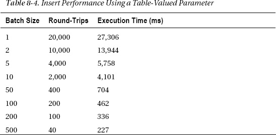
The performance isn’t as good as the previous example (sql-batch4.aspx) until the batch size reaches 50. However, unlike with the previous examples, in this case write performance continues to improve even if you increase the batch size to 500. The best performance here has more than 64 times the throughput of the original one-row-at-a-time example. A single row takes only about 11 microseconds to insert, which results in a rate of more than 88,000 rows per second.

Multiple Result Sets

If you need to process a number of queries at a time, each of which produces a separate result set, you can have SQL Server process them in a single round-trip. When executed, the command will return multiple result sets. This provides a mechanism to avoid issuing back-to-back queries separately; you should combine them into a single round-trip whenever possible.

You might do this by having a stored procedure that issues more than one SELECT statement that returns rows, or perhaps by executing more than one stored procedure in a batch, using the command batching techniques described earlier.

As an example, first create a stored procedure:

The procedure returns the first and last rows in the PageViews table, in two result sets, using a parameterized count.

Using SqlDataReader.NextResult()

Create a web form called sql-result1.aspx, add Async="True" to the Page directive, and edit the <form> part of the markup as follows:

The form has one text box for a count parameter, a submit button, and two data GridView controls.

Next, edit the code-behind, as follows:

The code executes the stored procedure and then binds each result set to a GridView control. Calling reader.NextResultAsync() after binding the first result set causes the reader to asynchronously advance to the next set of rows. This approach allows you to use a single round-trip to retrieve the two sets of rows generated by the stored procedure.

Using SqlDataAdapter and a DataSet

You can also use SqlDataAdapter to load more than one result set into multiple DataTables in a DataSet.

For example, make a copy of sql-result1.aspx called sql-result2.aspx, and edit the code-behind, as follows:

The call to adapter.Fill() will check to see whether more than one result set is available. For each result set, it will create and load one DataTable in the destination DataSet. However, this approach doesn’t work with asynchronous database calls, so it’s only suitable for background threads or perhaps infrequently used pages where synchronous calls are acceptable.

Data Precaching

As I mentioned earlier, after SQL Server reads data from disk into memory, the data stays in memory for a while; exactly how long depends on how much RAM is available and the nature of subsequent commands. This aspect of the database points the way to a powerful and yet rarely used performance optimization technique: precaching at the data tier.

Approach

In the cases where you can reasonably predict the next action of your users and where that action involves database access with predictable parameters, you can issue a query to the database that will read the relevant data into RAM before it’s actually needed. The goal is to precache the data at the data tier, so that when you issue the “real” query, you avoid the initial disk access. This can also work when the future command will be an UPDATE or a DELETE, since those commands need to read the associated rows before they can be changed.

Here are a few tips to increase the effectiveness of database precaching with a multiserver load-balanced web tier:

• You should issue the precache command either from a background thread or from an asynchronous Ajax call. You should not issue it in-line with the original page, even if the page is asynchronous.
• You should limit (throttle) the number precaching queries per web server to avoid unduly loading the server based solely on anticipated future work.
• Avoid issuing duplicate precaching queries.
• Don’t bother precaching objects that will probably already be in database memory, such as frequently used data.
• You should discard precaching queries if they are too old, since there’s no need to execute them after the target page has run.
• Execute precaching commands with a lower priority, using Resource Governor, so that they don’t slow down “real” commands.

Precaching Forms-Based Data

You may be able to use database precaching with some forms-based data. For example, consider a login page. After viewing that page, it’s likely that the next step for a user will be to log in, using their username and password. To validate the login, your application will need to read the row in the Users table that contains that user’s information. Since the index of the row you need is the user’s name and since you don’t know what that is until after they’ve started to fill in the form, Ajax can provide the first part of a solution here for precaching.

When the user exits the username box in the web form, you can issue an async Ajax command to the server that contains the user’s name. For precaching, you don’t care about the password, since the name alone will be enough to find the right row.

On the web server, the other side of the Ajax call would queue a request to a background thread to issue a SELECT to read the row of interest. The server will process that request while the user is typing their password. Although you might be tempted to return a flag from the Ajax call to indicate that the username is valid, that’s usually not recommended, for security reasons. In addition, the Ajax call can return more quickly if it just queues the request and doesn’t wait for a result.

When the user clicks the Login button on the web form, the code on the server will validate the username and password by reissuing a similar query. At that point, the data will already be in memory on the database server, so the query will complete quickly.

Precaching Page-at-a-Time Data

Another example would be paging through data, such as in a catalog. In that case, there may be a good chance that the user will advance to the next page after they finish viewing the current one. To make sure that the data for the next page are in memory on the database server, you could do something like this:

• Queue a work item to a background thread that describes the parameters to read the next page of data from the catalog and a timestamp to indicate when you placed the query in the queue.
• When the background thread starts to process the work item, it should discard the request if it’s more than a certain age (perhaps one to three seconds), since the user may have already advanced to the next page by then.
• Check the work item against a list of queries that the background thread has recently processed. If the query is on that list, then discard the request. This may be of limited utility in a load-balanced environment, but it can still help in the event of attacks or heavy burst-oriented traffic.
• Have the background thread use a connection to the server that’s managed by Resource Governor (see later in this chapter), so that the precaching queries from all web servers together don’t overwhelm database resources. That can also help from a security perspective by minimizing the impact of a denial-of-service attack.
• Cache the results of the query at the web tier, if appropriate.
• After issuing the query, the background thread might sleep for a short time before retrieving another work item from the queue, which will throttle the number of read-ahead requests that the web server can process.

The performance difference between using data that’s already in memory and having to read it from disk first can be very significant – as much as a factor of ten or even much more, depending on the size of the data, the details of the query and the associated schema, and the speed of your disk subsystem.

Data Access Layer

An often-cited best practice for data-oriented applications is to provide a layer of abstraction on top of your data access routines. That’s usually done by encapsulating them in a data access layer (DAL), which can be a class or perhaps one or more assemblies, depending on the complexity of your application.

The motivations for grouping the data access code in one place include easing maintenance, database independence (simplifying future migration to other data platforms), encouraging consistent patterns, maximizing code reuse, and simplifying management of command batches, connections, transactions, and multiple result sets.

With synchronous database commands, the DAL methods would typically execute the command and return the result. If you use asynchronous commands everywhere you can, as I suggested in earlier chapters, you will need to modify your DAL accordingly.

For the Asynchronous Programming Model (APM), in the same style as the ADO.NET libraries, you should divide your code into one method that begins a query and another that ends it and collects the results.

Here’s an example:

The AddBrowserBegin() method creates a SqlConnection from an async connection string, along with an associated SqlCommand. After filling in the parameters, it opens the connection, begins the command, and returns the resulting IAsyncResult.

The AddBrowserEnd() method ends the command and calls Dispose() on the SqlConnection and SqlCommand objects (implicitly via a using statement for SqlCommand and explicitly for SqlConnection).

For the Task-based Asynchronous Pattern (TAP), it only takes a single method; you can simplify the code considerably:

You will probably also want to include connection and transaction management in your DAL. ADO.NET uses connection pools to reuse connections as much as it can. Connections are pooled based entirely on a byte-for-byte comparison of the connection strings; different connection strings will not use connections from the same pool. However, even with identical connection strings, if you execute a command within the scope of one SqlConnection object and then execute another command within the scope of a different SqlConnection, the framework will treat that as a distributed transaction. To avoid the associated performance impact and complexity, it’s better to execute both commands within the same SqlConnection. In fact, it would be better still to batch the commands together, as described earlier. Command batching and caching are also good things to include in your DAL.

Query and Schema Optimization

There’s a definite art to query and schema optimization. It’s a large subject worthy of a book of its own, so I’d like to cover just a few potentially high-impact areas.

Clustered and Nonclustered Indexes

Proper design of indexes, and in particular the choice between clustered and nonclustered indexes and their associated keys, is critical for optimal performance of your database.

As I mentioned earlier, SQL Server manages disk space in terms of 8KB pages and 64KB extents. When a clustered index is present, table rows within a page and the pages within an extent are ordered based on that index. Since a clustered index determines the physical ordering of rows within a table, each table can have only one clustered index.

A table can also have secondary, or nonclustered, indexes. You can think of a nonclustered index as a separate table that only has a subset of the columns from the original table. You specify one or more columns as the index key and they will determine the physical order of the rows in the index. By default, the rows in a nonclustered index only contain the key and the clustered index key, if there is one and if it’s unique. However, you can also include other columns from the table.

A table without any indexes is known as a heap and is unordered.

Neither a clustered nor a nonclustered index has to be unique or non-null, though both can be. Of course, both types of indexes can also include multiple columns, and you can specify an ascending or descending sort order. If a clustered index is not unique, then all nonclustered indexes include a 4-byte pointer back to the original row, instead of the clustered index.

Including the clustered index key in the nonclustered index allows SQL Server to quickly find the rest of the columns associated with a particular row, through a process known as a key lookup. SQL Server may also use the columns in the nonclustered index to satisfy the query; if all the columns you need to satisfy your query are present in the nonclustered index, then the key lookup can be skipped. Such a query is covered. You can help create covered queries and eliminate key lookups by adding the needed columns to a nonclustered index, assuming the additional overhead is warranted.

Index Performance Issues

Since SQL Server physically orders rows by the keys in your indexes, consider what happens when you insert a new row. For an ascending index, if the value of the index for the new row is greater than that for any previous row, then it is inserted at the end of the table. In that case, the table grows smoothly, and the physical ordering is easily maintained. However, if the key value places the new row in the middle of an existing page that’s already full of other rows, then that page will be split by creating a new one and moving half of the existing rows into it. The result is fragmentation of the table; its physical order on disk is no longer the same as its logical order. The process of splitting the page also means that it is no longer completely full of data. Both of those changes will significantly decrease the speed with which you will be able to read the full table.

The fastest way for SQL Server to deliver a group of rows from disk is when they are physically next to each other. A query that requires key lookups for each row or that even has to directly seek to each different row will be much slower than one that can deliver a number of contiguous rows. You can take advantage of this in your index and query design by preferring indexes for columns that are commonly used in range-based WHERE clauses, such as BETWEEN.

When there are indexes on a table, every time you modify the table, the indexes may also need to be modified. Therefore, there’s a trade-off between the cost of maintaining indexes and their use in allowing queries to execute faster. If you have a table where you are mostly doing heavy INSERTs and only very rarely do a SELECT, then it may not be worth the performance cost of maintaining an extra index (or any index at all).

If you issue a query with a column in the WHERE clause that doesn’t have an index on it, the result is usually either a table scan or an index scan. SQL Server reads every row of the table or index. In addition to the direct performance cost of reading every row, there can also be an indirect cost. If your server doesn’t have enough free memory to hold the table being scanned, then buffers in the cache will be dropped to make room, which might negatively affect the performance of other queries. Aggregation queries, such as COUNT and SUM, by their nature often involve table scans, and for that reason, you should avoid them as much as you can on large tables. See the next chapter for alternatives.

Index Guidelines

With these concepts in mind, here are some guidelines for creating indexes:

• Prefer narrow index keys that always increase in value, such as an integer IDENTITY. Keeping them narrow means that more rows will fit on a page, and having them increase means that new rows will be added at the end of the table, avoiding fragmentation.
• Avoid near-random index keys such as strings or UNIQUEIDENTIFIERs. Their randomness will cause a large number of page splits, resulting in fragmentation and associated poor performance.
• Although exact index definitions may evolve over time, begin by making sure that the columns you use in your WHERE and JOIN clauses have indexes assigned to them.
• Consider assigning the clustered index to a column that you often use to select a range of rows or that usually needs to be sorted. It should be unique for best performance.
• In cases where you have mostly INSERTs and almost no SELECTs (such as for logs), you might choose to use a heap and have no indexes. In that case, SQL Server will insert new rows at the end of the table, which prevents fragmentation. That allows INSERTs to execute very quickly.
• Avoid table or index scans. Some query constructs can force a scan even when an index is available, such as a LIKE clause with a wildcard at the beginning.

Although you can use NEWSEQUENTIALID() to generate sequential GUIDs, that approach has some significant limitations:

• It can be used only on the server, as the DEFAULT value for a column. One of the more useful aspects of GUIDs as keys is being able to create them from a load-balanced web tier without requiring a database round-trip, which doesn’t work with this approach.
• The generated GUIDs are only guaranteed to be increasing for “a while.” In particular, things like a server reboot can cause newly generated GUIDs to have values less than older ones. That means new rows aren’t guaranteed to always go at the end of tables; page splits can still happen.
• Another reason for using GUIDs as keys is to have user-visible, non-guessable values. When the values are sequential, they become guessable.

Example with No Indexes

Let’s start with a table by itself with no indexes:

The table has three columns: an integer IDENTITY, another integer, and a string. Since it doesn’t have any indexes on it yet, this table is a heap. INSERTs will be fast, since they won’t require any validations for uniqueness and since the sort order and indexes don’t have to be maintained.

Next, let’s add a half million rows to the table, so you’ll have a decent amount of data to run test queries against:

The v1 IDENTITY column will automatically be filled with integers from 1 to 500,000. The v2 column will contain even integers from zero to one million, and the v3 column will contain a fixed string. Of course, this would be faster if you did multiple inserts in a single transaction, as discussed previously, but that’s overkill for a one-time-only script like this.

You can have a look at the table’s physical characteristics on disk by running the following command:

Since there are no indexes yet, information is displayed for the table only:

You can see from this that the table occupies 1,624 pages and 204 extents and that the pages are 95.07 percent full on average.

Adding a Clustered Index

Here’s the first query that you’re going to optimize:

You’re retrieving all three columns from a range of rows, based on the v1 IDENTITY column.

Before running the query, let’s look at how SQL Server will execute it. Do that by selecting it in SSMS, right-clicking, and selecting Display Estimated Execution Plan. Here’s the result:

This shows that the query will be executed using a table scan; since the table doesn’t have an index yet, the only way to find any specific values in it is to look at each and every row.

Before executing the query, let’s flush all buffers from memory:

The CHECKPOINT command tells SQL Server to write all the dirty buffers it has in memory out to disk. Afterward, all buffers will be clean. The DBCC DROPCLEANBUFFERS command then tells it to let go of all the clean buffers. The two commands together ensure that you’re starting from the same place each time: an empty buffer cache.

Next, enable reporting of some performance-related statistics after running each command:

STATISTICS IO will tell you how much physical disk I/O was needed, and STATISTICS TIME will tell you how much CPU time was used.

Run the query, and click the Messages tab to see the reported statistics:

The values you’re interested in are 29 physical reads, 1,624 read-ahead reads, 141ms of CPU time, and 348ms of elapsed time. Notice that the number of read-ahead reads is the same as the total size of the table, as reported by DBCC SHOWCONTIG in the previous code listing. Also notice the difference between the CPU time and the elapsed time, which shows that the query spent about half of the total time waiting for the disk reads.

The fact that the query is looking for the values of all columns over a range of the values of one of them is an ideal indication for the use of a clustered index on the row that’s used in the WHERE clause:

Since the v1 column is an IDENTITY, that means it’s also UNIQUE, so you include that information in the index. This is almost the same as SQL Server’s default definition of a primary key from an index perspective, so you can accomplish nearly the same thing as follows:

The difference between the two is that a primary key does not allow NULLs, where the unique clustered index does, although there can be only one row with a NULL when the index is unique.

Repeating the DBCC SHOWCONTIG command now shows the following relevant information:

There are a few less pages and extents, with a corresponding increase in page density.

After adding the clustered index, here’s the resulting query plan:

The table scan has become a clustered index seek, using the newly created index.

After flushing the buffers again and executing the query, here are the relevant statistics:

The total number of disk reads has dropped from 1,624 to just 3, CPU time has decreased from 141ms to less than 1ms, and elapsed time has decreased from 348ms to 33ms. At this point, our first query is fully optimized.

Adding a Nonclustered Index

Here’s the next query:

This is similar to the previous query, except it’s using v2 in the WHERE clause instead of v1.

Here’s the initial query plan:

This time, instead of scanning the table, SQL Server will scan the clustered index. However, since each row of the clustered index contains all three columns, this is really the same as scanning the whole table.

Next, flush the buffers again, and execute the query. Here are the results:

Sure enough, the total number of disk reads still corresponds to the size of the full table. It’s a tiny bit faster than the first query without an index, but only because the number of pages decreased after you added the clustered index.

To speed up this query, add a nonclustered index:

As with the first column, this column is also unique, so you include that information when you create the index.

Running DBCC SHOWCONTIG now includes information about the new index:

You can see that it’s a little more than half the size of the clustered index. It’s somewhat smaller since it only includes the integer v1 and v2 columns, not the four-character-long strings you put in v3.

Here’s the new query plan:

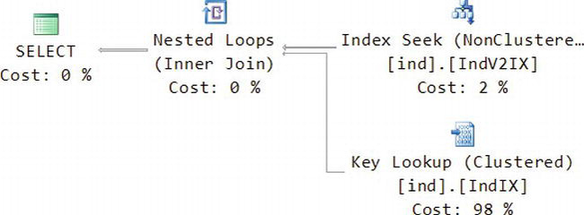
This time, SQL Server will do an inexpensive index seek on the IndV2IX nonclustered index you just created. That will allow it to find all the rows with the range of v2 values that you specified. It can also retrieve the value of v1 directly from that index, since the clustered index column is included with all nonclustered indexes. However, to get the value of v3, it needs to execute a key lookup, which finds the matching row using the clustered index. Notice too that the key lookup is 98 percent of the cost of the query.

The two indexes amount to two physically separate tables on disk. The clustered index contains v1, v2, and v3 and is sorted and indexed by v1. The nonclustered index contains only v1 and v2 and is sorted and indexed by v2. After retrieving the desired rows from each index, the inner join in the query plan combines them to form the result.

After flushing the buffers again and executing the query, here are the results:

The CPU time and elapsed time are comparable to the first query when it was using the clustered index. However, there are more disk reads because of the key lookups.

Creating a Covered Index

Let’s see what happens if you don’t include v3 in the query:

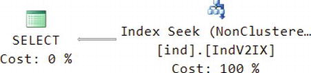
Here’s the query plan:

Since you don’t need v3 any more, now SQL Server can just use an index seek on the nonclustered index.

After flushing the buffers again, here are the results:

You’ve eliminated the extra disk reads, and the elapsed time has dropped significantly too.

You should be able to achieve a similar speedup for the query that uses v3 by adding v3 to the nonclustered index to create a covered index and avoid the key lookups:

This command will include v3 in the existing index, without having to separately drop it first.

Here’s the updated DBCC SHOWCONTIG for the nonclustered index:

The index has grown from 866 pages and 109 extents to 1,359 pages and 170 extents, while the page density remains close to 100 percent. It’s still a little smaller than the clustered index because of some extra information that is stored in the clustered index other than just the column data.

The new query plan for the original query with v3 that you’re optimizing is exactly the same as the plan shown earlier for the query without v3:

Here are the statistics:

The results are also the same as the previous test. However, the price for this performance is that you now have two complete copies of the table: one with v1 as the index, and one with v2 as the index. Therefore, while SELECTs of the type you used in the examples here will be fast, INSERTs, UPDATEs, and DELETEs will be slower, because they now have to change two physical tables instead of just one.

Index Fragmentation

Now let’s see what happens if you insert 5,000 rows of data that has a random value for v2 that’s in the range of the existing values, which is between zero and one million. The initial values were all even numbers, so you can avoid uniqueness collisions by using odd numbers. Here’s the T-SQL:

Those 5,000 rows are 1 percent of the 500,000 rows already in the table. After running the script, here’s what DBCC SHOWCONTIG reports for the clustered index:

For the nonclustered index, it reports the following:

Notice that the clustered index has just a few more pages and extents, and it remains at close to 100 percent page density. However, the nonclustered index has gone from 1,359 pages and 170 extents at close to 100 percent density to 2,680 pages, 339 extents, and about 50 percent density. Since the clustered index doesn’t depend on the value of v2 and since v1 is an IDENTITY value that steadily increases, the new rows can just go at the end of the table.

Rows in the nonclustered index are ordered based on v2. When a new row is inserted, SQL Server places it in the correct page and position to maintain the sort order on v2. If that results in more rows than will fit on the page, then the page is split in two, and half the rows are placed in each page. That’s why you see the average page density at close to 50 percent.

Excessive page splits can have a negative impact on performance, since they can mean that many more pages have to be read to access the same amount of data.

You can explicitly defragment the indexes for the ind table with the following command:

COLUMNSTORE Index

SQL Server 2012 introduced a new, special purpose type of index called COLUMNSTORE, available only in the Enterprise and Developer editions. COLUMNSTORE indexes improve the efficiency of index scans. They’re useful in scenarios where you have very large tables (generally multiple millions of rows) that you often query using joins and aggregates, such as with a fact table in a data warehouse.

One downside of COLUMNSTORE indexes is that they cause your table to become read-only. Limited modification is possible without dropping and re-creating the index on the entire table, but it requires using data partitioning (covered later in this chapter) to switch out part of the table.

The upside of COLUMNSTORE indexes is that they can provide a very significant performance boost for certain types of queries. Scans of even billions of rows can complete in a few seconds or less.

As the name implies, COLUMNSTORE indexes organize data by columns, rather than by rows as in a conventional index. The indexes don’t have a particular order. SQL Server compresses the rows within each column after first re-ordering them to optimize the amount of compression that’s possible.

As an example, let’s optimize the following query, which uses a table scan:

Here are the initial statistics:

Create the index:

It’s a sound practice to include all of the eligible columns of your table in the index. There are several data types you can’t use in a COLUMNSTORE index: BINARY, VARBINARY, IMAGE, TEXT, NTEXT, VARCHAR(MAX), CURSOR, HIERARCHYID, TIMESTAMP, UNIQUEIDENTIFIER, SQLVARIANT, XML, DECIMAL or NUMERIC with precision larger than 18, and DATETIMEOFFSET with precision greater than 2.

Here are the statistics after repeating the query with the index in place:

Due to the high compressibility of the data (all rows contain the same value of v3), the query only requires three physical disk reads for the index, compared to 1,597 reads without the index. CPU time and elapsed time are also much lower.

Miscellaneous Query Optimization Guidelines

Here are a few high-level guidelines for optimizing your queries:

• If you’re writing new queries or code that invokes queries, you should make frequent and regular use of the SQL Profiler to get a feeling for how many round-trips your code is making and how long the queries are taking. For me, it plays an irreplaceable role when I’m doing that kind of work.
• Avoid cursors. Processing data a row-at-a-time in T-SQL is very expensive. Although there are exceptions, 99 percent of the time, it’s worth the effort to rewrite your queries to use set-based semantics, if possible. Alternatives include things like table variables, temporary tables, and so on. I’ve rewritten some cursor-based queries that ran 1,000 times faster as set-based operations. If you can’t avoid cursors, identify all read-only queries, and mark the associated cursors as FAST_FORWARD.
• Avoid triggers. Triggers are a powerful tool, but you should think of them as a last resort; use them only if there is no other way. They can introduce massive amounts of overhead, which tends to be of the slow, row-at-a-time type. Because triggers are nominally hidden from the view of developers, what’s worse is that the extra overhead is hidden too.
• To avoid performance problems because of deadlocks, make a list of all the stored procedures in your system and the order in which they modify tables, and work to ensure that order is consistent from one stored procedure to another. In cases where consistent order isn’t possible, either use an increased transaction isolation level or use locking hints or increased lock granularity.
• Use SET NOCOUNT ON at the top of most of your stored procedures to avoid the extra overhead of returning a result row count. However, when you want to register the results of a stored procedure with SqlDependency or SqlCacheDependency, then you must not use SET NOCOUNT ON. Similarly, some of the logic that synchronizes DataSets uses the reported count to check for concurrency collisions.

Data Paging

If you have a large database table and you need to present all or part of it to your users, it can be painfully slow to present a large number of rows on a single page. Imagine a user trying to scroll through a web page with a million rows on it. Not a good idea. A better approach is to display part of the table. While you’re doing so, it’s also important to avoid reading the entire table at both the web tier and the database tier.

Common Table Expressions

You can use common table expressions (CTEs) to address this issue (among many other cool things). Using the PageViews table from the beginning of the chapter as an example, here’s a stored procedure that returns only the rows you request, based on a starting row and a page size:

The query works by first declaring an outer frame, including a name and an optional list of column names, in this case, ViewList ([row], [date], [user], [url]).

Next, you have a query that appears to retrieve all the rows in the table, while also applying a row number, using the ROW_NUMBER() function, with which you need to specify the column you want to use as the basis for numbering the rows. In this case, you’re using OVER (ORDER BY PvId). The columns returned by this query are the same ones listed in the outer frame. It might be helpful to think of this query as returning a temporary result set.

Although the ROW_NUMBER() function is very handy, unfortunately you can’t use it directly in a WHERE clause. This is what drives you to using a CTE in the first place, along with the fact that you can’t guarantee that the PvId column will always start from one and will never have gaps.

Finally, at the end of the CTE, you have a query that references the outer frame and uses a WHERE clause against the row numbers generated by the initial query to limit the results to the rows that you want to display. SQL Server only reads as many rows as it needs to satisfy the WHERE clause; it doesn’t have to read the entire table.

OFFSET

SQL Server 2012 introduced an alternative approach to CTEs for data paging that’s much easier to use: OFFSET.

For example:

OFFSET requires an ORDER BY clause. An OFFSET of zero produces the same results as TOP.

Detailed Example of Data Paging

To demonstrate data paging in action, let’s build an example that allows you to page through a table and display it in a GridView control.

Markup

First, add a new web form to your web site, called paging.aspx, and edit the markup as follows:

Here you’re using several of the best practices discussed earlier: both ViewState and AutoEventWireup are disabled.

In the GridView control, enable AllowPaging, set the PageSize, and associate the control with a data source. Since you want to use the control’s paging mode, using a data source is required. Use the <PagerSettings> tag to customize the page navigation controls a bit.

Use an ObjectDataSource as the data source, since you want to have programmatic control over the details. Set EnablePaging here, associate the control with what will be your new class using TypeName, and set a SelectMethod and a SelectCountMethod, both of which will exist in the new class. The control uses SelectMethod to obtain the desired rows and SelectCountMethod to determine how many total rows there are so that the GridView can correctly render the paging navigation controls. Also, set OnObjectCreated and OnObjectDisposing event handlers.

Stored Procedure

Next, use SSMS to modify the stored procedure that you used in the prior example as follows:

Rather than requiring a separate round trip to determine the number of rows in the table, what the example does instead is to add a flag to the stored procedure, along with an output parameter. The T-SQL incurs the overhead of running the SELECT COUNT(*) query (which requires a table scan) only if the flag is set, and returns the result in the output parameter.

Code-Behind

Next, edit the code-behind as follows:

Since AutoEventWireup is disabled, override the OnEvent-style methods from the base class.

The ObjectDataSource control needs to know how many rows there are in the target table. Obtaining the row count is expensive; counting rows is a form of aggregation query that requires reading every row in the table. Since the count might be large and doesn’t change often, you should cache the result after you get it the first time to avoid having to repeat that expensive query.

You could use the Cache object if you access the count frequently from multiple pages. In a load-balanced environment, a different server might process the request for the next page, and it wouldn’t have the access to the same cache. You could use a cookie, but they are a bit heavyweight for information that’s specific to a single page. For data that’s specific to a page like this, ViewState might be a good choice. However, on this page, you would like to keep ViewState disabled because it gets very voluminous for the GridView control and therefore has an associated negative effect on page performance. You could enable ViewState on the page and just disable it for the GridView control, but leaving it enabled for other controls will make the page larger than it has to be. Instead, let’s use ControlState, which serves a purpose similar to ViewState, except that it can’t be disabled.

In OnInit(), call RegisterRequiresControlState() to inform the Page class that you will be using ControlState.

If the current request isn’t a postback, that means a user is coming to the page for the first time, and you will need to obtain the row count. If the request is a postback, then you will obtain the row count from ControlState.

Unlike with ViewState, which uses a Dictionary as its primary interface, with ControlState you have to override the LoadControlState() and SaveControlState() methods instead. LoadControlState() is called before the Load event, and SaveControlState() is called after the PreRender event. As with ViewState, ControlState is encoded and stored in the __VIEWSTATE hidden field in your HTML.

The runtime will call the ObjectCreated event handler after creating an instance of the Sample.PageViews object. Use this event to push the row count into the object.

The runtime will call the ObjectDisposing event handler after it has done its work. Use this event to retrieve the (possibly updated) row count from the object, so that you can cache it on the page.

Object Data Source

Next is the object data source, which is the final class for the example. Add a file for a new class called PageViews.cs to your project in the App_Code folder:

Call the stored procedure to obtain the row count (if needed) using an output parameter, along with the requested rows. This logic relies on the fact that the runtime calls GetRows() before GetCount(), since the count reported by the latter is obtained (the first time) from the former.

Results

The resulting web page still needs some work to pretty it up, but it’s definitely functional. Equally important, it’s also very scalable, even on extremely large tables. It uses an efficient query for paging, caches the row count in ControlState so the count query doesn’t need to be executed again for every new page viewed by the same user, and always uses only one round-trip to the database.

Figure 8-1 shows part of page 11 of the output, including the column headers and the navigation links.

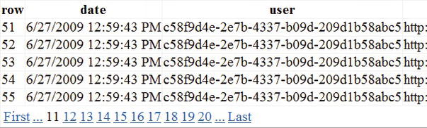
Figure 8-1. Output from the paging GridView example

LINQ to SQL, Entity Framework and other ORMs

Language Integrated Query (LINQ) was one of the very cool additions to C# 3.0. It provides a type-safe way to query XML, SQL Server, and even your own objects. LINQ to SQL also provides a mapping from database objects (tables and rows) to .NET objects (classes). That allows you to work with your custom business objects, while delegating much of the work involved with synchronizing those objects to LINQ.

The Entity Framework (EF) is an alternative to LINQ to SQL, which you can also query with LINQ. NHibernate is an open source system that provides similar functionality.

All of these systems provide an Object Relational Model (ORM), each with its own pros and cons. I have mixed feelings about all ORM systems. I love them because they allow me to develop small, proof-of-concept sites extremely quickly. I can side step much of the SQL and related complexity that I would otherwise need and focus on the objects, business logic and presentation. However, at the same time, I also don’t care for them because, unfortunately, their performance and scalability is usually very poor, even when they’re integrated with comprehensive caching – which isn’t always easy or even straightforward.

The object orientation of ORM systems very often results in extremely chatty implementations. Because ORM systems tend to make it a little too easy to access the database, they often result in making many more round-trips than you really need. I’ve seen sites that average more than 150 round-trips to the database per page view! Overall, databases are more efficient at handling set-based operations than per-object (row-at-a-time) operations.

Although both LINQ and NHibernate’s hql do provide some control over the queries that are autogenerated by these systems, in complex applications the queries are often inefficient and difficult or impossible to tune fully. In addition, in their current incarnations, LINQ to SQL and the Entity Framework don’t provide good support for asynchronous requests, command batching, caching, or multiple result sets, which are all important for scalable high-performance databases.

You can also use stored procedures with ORM systems, although you do sacrifice some flexibility in doing so.

Of course, I understand that ORM systems have become extremely popular, largely because of their ease of use. Even so, in their current form I can’t recommend any of them in high-performance web sites, in spite of how unpopular that makes me in some circles. LINQ is great for querying XML and custom objects; I just would prefer not to use it or EF with SQL, except in very limited circumstances, such as:

• Rapid prototyping or proofs of concept, where speed of delivery is more important than performance and scalability (beware of the tendency for successful prototypes to move to production without an opportunity for a complete rewrite).
• Small-scale projects.
• As an alternative to generating dynamic SQL by concatenating strings on the web tier when you can’t otherwise avoid it.
• As a way of calling stored procedures synchronously with type-safe parameters, such as from a background thread or a Windows service.
• Isolated, low-traffic, low-load parts of a site.

I’m definitely not saying that working with objects is a bad idea; it’s the T-SQL side of things that presents difficulties. You can fill a collection of custom objects yourself very quickly and efficiently by using a SqlDataReader; that’s what the SqlDataAdapter and DataTable objects do. If you need change detection, you can use a DataSet (which can contain one or more DataTables). However, that is a fairly heavyweight solution, so custom objects are usually the most efficient approach.

From a performance perspective, if you’re using the LinqDataSource control, it helps if you can include a TIMESTAMP column in the associated tables. If a table doesn’t have a TIMESTAMP column, the control checks data concurrency by storing the original data values on the page. LINQ to SQL verifies that the row still contains the original values before it updates or deletes data. This approach can result in an unnecessarily large page, as well as presenting potential security issues. If the table has a TIMESTAMP column, then the control stores only that value on the page. LINQ to SQL can verify data consistency by checking whether the original TIMESTAMP matches the current one.

XML Columns

SQL Server 2005 introduced the ability to store XML data as a native data type. Before that, the alternative was to store it as a blob of text. With XML native columns, you can efficiently query or modify individual nodes in your XML. This feature is useful from a performance perspective in several scenarios:

• As a replacement for sparse columns. Rather than having a very wide table where most of the values are NULL, you can have a single XML column instead.
• When you need recursive or nested elements or properties that are difficult to represent relationally.
• When you have existing XML documents that you would like to be able to query or update, while retaining their original structure.
• As an alternative to dynamically adding new columns to your tables. Adding new columns to a table will lock the table while the change is in progress, which can be an issue for very large tables. Adding new columns can also be challenging to track with respect to their impact on existing queries and indexes.
• As an alternative to many-to-many mappings. In cases where a relational solution would include extra tables with name/value pairs and associated mappings and indexes, native XML columns can provide a more flexible solution that avoids the overhead of joining additional tables.

Before going any further, I should say that if your data fits the relational model well, then you should use a relational solution. Only consider XML when relational becomes difficult, awkward, or expensive from a performance perspective, as in the examples I listed earlier. Avoid the temptation to convert your entire schema to XML, or you will be very disappointed when it comes to performance!

XML columns have their own query language, separate from (although integrated with) T-SQL, called XQuery. Rather than diving into its full complexities, let’s walk through a couple of examples to give you a sense of what it’s like, along with a few performance tips.

XML Schema

Let’s build a table of products. The product name is always known, so you’ll put that in a relational column. Each product can also have a number of attributes. You expect that the number and variety of attributes will expand over time and that they might have a recursive character to them, so you decide to represent them in XML and include them in an XML column in the products table.

Here’s an example of what the initial XML will look like:

SQL Server can associate a collection of XML schemas with an XML column. Although the use of schemas is optional, they do have a positive impact on performance. Without a schema, XML is stored as a string and is parsed for each access. When a schema is present, the XML is converted to binary, which reduces its size and makes it faster to query. In addition, numeric values are stored in their converted form. Without a schema, SQL Server can’t tell the difference between an item that should be a string and one that should be a number, so it stores everything as strings.

Since schemas are a good thing, let’s create one that describes our XML and create a schema collection to go with it:

This schema encodes the rules for the structure of your XML: inside an outer info element, the optional <props> element has optional width and depth attributes. There can be zero or more <color> elements, each of which has a required part attribute and a string that describes the color. If it’s present, the <props> element must come before the <color> elements (<xs:sequence>).

XML schemas can get complex quickly, so I recommend using some software to accelerate the process and to reduce errors. Since the market changes frequently, see my links page at www.12titans.net/p/links.aspx for current recommendations.

Creating the Example Table

Now you’re ready to create the table:

You have an integer IDENTITY column as a PRIMARY KEY, a string for the product name, and an XML column to hold extra information about the product. You have also associated the ProductSchema schema collection with the XML column.

Next, insert a few rows into the table:

You might also try inserting rows that violate the schema to see the error that SQL Server returns.

Basic XML Queries

A simple query against the table will return the Info column as XML:

Now let’s make some queries against the XML:

The exist() clause is equal to 1 for rows where the XML has a props element with a width attribute. The query() in the selected columns will display the props element and its attributes (and children, if it had any) as XML; it’s a way to show a subset of the XML.

Both query() and exist() use XPath expressions, where elements are separated by slashes and attributes are in brackets preceded by an at-sign.

Here’s another query:

This time, you’re looking for all rows where <color part="top"> is set to black. The value() query lets you convert an XQuery/XML value to a T-SQL type so you can compare it against black. In the selected columns, use value() to return the width attribute of the props element. Converting it to a T-SQL type means that the returned row set has the appearance of being completely relational; there won’t be any XML, as there was in the previous two queries. Since the XPath expressions might match more than one node in the XML, the [1] in both value() queries says that you’re interested in the first match; value() requires you to limit the number of results to just one.

Here’s the next query:

This time, you’re using the sql:variable() function to integrate the @part variable into the XQuery. You would use this approach if you wanted to parameterize the query, such as in a stored procedure. On the results side, you’re returning the first color in the list.

Modifying the XML Data

In addition to being able to query the XML data, you can also modify it:

This command will set the value of the <color part="legs"> element for the Desk Chair row to silver.

This command inserts a new color element at the beginning of the list. Notice that a T-SQL UPDATE statement is used to do this type of insert, since you are changing a column and not inserting a new row into the table.

This command deletes the first color element in the list, which is the same one that you just inserted with the previous command.

XML Indexes

As with relational data, you can significantly improve the performance of queries against XML if you use the right indexes. XML columns use different indexes than relational data, so you will need to create them separately:

A PRIMARY XML INDEX is, as the name implies, the first and most important XML index. It contains one row for every node in your XML, with a clustered index on the node number, which corresponds to the order of the node within the XML. To create this index, the table must already have a primary key. You can’t create any of the other XML indexes unless the PRIMARY XML INDEX already exists.

You create the remaining three indexes in a similar way, using either FOR PATH, FOR PROPERTY, or FOR VALUE. These secondary indexes are actually nonclustered indexes on the node table that comprises the primary index. The PATH index includes the tokenized path of the node and its value. The PROPERTY index includes the original table’s primary key plus the same columns as the path index. The VALUE index has the value first, followed by the tokenized path (the inverse of the PATH index).

Each index is useful for different types of queries. Because of the complexity of both the indexes and typical queries, I’ve found that the best approach for deciding which indexes to generate is to look carefully at your query plans. Of course, if your data is read-only and you have plenty of disk space, then you might just create all four indexes and keep things simple. However, if you need to modify or add to your data, then some analysis and testing is a good idea. XML index maintenance can be particularly expensive; the entire node list for the modified column is regenerated after each change.

Miscellaneous XML Query Tips

Here are a few more tips for querying XML:

• Avoid wildcards, including both the double-slash type (//) and the asterisk type.
• Consider using full-text search, which can find strings much more efficiently than XQuery. One limitation is that it doesn’t understand the structure of your XML, so it ignores element and attribute names.
• If you search against certain XML values very frequently, consider moving them into a relational column. The move can be either permanent or in the form of a computed column.
• You may be able to reduce the coding effort required to do complex joins by exposing relevant data as relational columns using views.

Data Partitioning

Working with very large tables often presents an interesting set of performance issues. Here’s an example:

• Certain T-SQL commands can lock the table. If those commands are issued frequently, they can introduce delays because of blocking.
• Queries can get slower as the table grows, particularly for queries that require table or index scans.
• If the table grows quickly, you will probably want to delete part of it eventually, perhaps after archiving it first. Deleting the data will place a heavy load on the transaction log, since SQL Server will write all the deleted rows to the log.
• If the table dominates the size of your database, it will also drive how long it takes to do backups and restores.

SQL Enterprise and Developer editions have a feature called table partitioning that can help address these problems. The way it works is that first you define one or more data value borders that are used to determine in which partition to place each row. Partitions are like separate subtables; they can be locked separately and placed on separate filegroups. However, from a query perspective, they look like a single table. You don’t have to change your queries at all after partitioning a table; SQL Server will automatically determine which partitions to use.

You can also switch a partition from one table to another. After the change, you can truncate the new table instead of deleting it, which is a very fast process that doesn’t overwhelm the database log.

Partition Function

Let’s walk through a detailed example with the same PageViews table that you used earlier. Let’s say that the table grows quickly and that you need to keep data for only the last few months online for statistics and reporting purposes. At the beginning of each month, the oldest month should be deleted. If you just used a DELETE command to delete the oldest month, it would lock the table and make it inaccessible by the rest of your application until the command completes. If your site requires nonstop 24×7 operations, this type of maintenance action can cause your system to be slow or unresponsive during that time. You can address the issue by partitioning the table by month.

The first step is to create a PARTITION FUNCTION:

The command specifies the data type of the column against which you will be applying the partition function. In this case, that’s DATETIME. Specifying RANGE RIGHT says that the border values will be on the right side of the range.

The values are dates that define the borders. You’ve specified nine values, which will define ten partitions (N + 1). Since you’re using RANGE RIGHT, the first value of 20090101 defines the right side of the border, so the first partition will hold dates less than 01 Jan 2009. The second value of 20090201 says that the second partition will hold dates greater than 01 Jan 2009 and less than 01 Feb 2009. The pattern repeats up to the last value, where an additional partition is created for values greater than 01 Sep 2009.

Partition Scheme

Next, create a PARTITION SCHEME, which defines how the PARTITION FUNCTION maps to filegroups:

In this case, place all the partitions on the PRIMARY filegroup. Multi-filegroup mappings can be appropriate in hardware environments where multiple LUNs or logical drives are available to help spread the I/O load.

At this point, you can use the $partition function along with the name of the PARTITION FUNCTION as defined earlier to test the assignment of partition values to specific partitions:

That query displays 3, which indicates that a row with a partition value of 20090215 would be assigned to partition number 3.

Now you’re ready to create the table:

Assign the ByMonthPS partition scheme to the table with the ON clause at the end of the definition, along with the column, PvDate, that SQL Server should use with the partition function.

Generating Test Data

At this point, you’re ready to generate some test data.

Some editions of Visual Studio include an automated data generation tool. However, in a case like this, where we mainly need to generate random data for one field, a T-SQL script can offer a little more flexibility (in part because it doesn’t require Visual Studio to develop or run the script):

The call to RAND(1) sets a seed for the random number generator that carries through the rest of the script. That means you can reproduce the exact results you see here, and they will stay the same from one run to another.

You generate random a random DATETIME field by first computing the number of seconds between 01-Oct-2008 and 05-Jul-2009, which overlaps the partition definition function from earlier. Then add a random number of seconds between zero and that number to the lower end of the range, and INSERT that value into the table.

NEWID() generates a new GUID for each call, and you’re using a fixed value for the PvUrl column.

In keeping with the earlier discussion about inserting multiple rows per transaction for best performance, you have an inner loop that inserts 1,000 rows for each transaction, and an outer loop that executes 500 of those transactions, for a total of 500,000 rows. Using transactions in this way reduces the run time on my machine from 63 seconds to 9 seconds.

Adding an Index and Configuring Lock Escalation

Now you’re ready to add an index:

If you have a clustered key, the column you use for partitioning must also be present in the key, so you include PvDate in addition to PvId. If you try to exclude PvDate from the key, you’ll get an error.

Let’s also configure the table so that when needed, SQL Server will escalate locks up to the heap or B-tree granularity, rather than to the full table:

That can help reduce blocking and associated delays if you’re using commands that require table locks.

To see the results of partitioning the test data, run the following query:

See Figure 8-2 for the results.

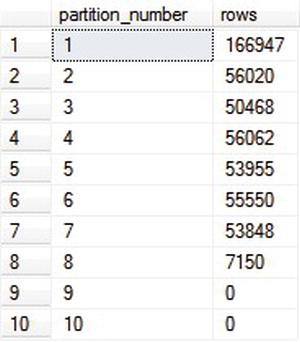
Figure 8-2. Results of data partitioning after test data generation

Partitions 2 through 8 have roughly the same number of rows, covering one month each. Partition 1 has more than the average, because it includes several months (01-Oct-2008 to 31-Dec-2008), based on the lower end of the date range you used for the test data. Partition 8 has less than the average, since the high end of the range (05-Jul-2009) didn’t include an entire month.

Archiving Old Data

Let’s get ready to archive the old data. First, create a table with the same schema and index as the source table:

Although it’s not a strict requirement, I’ve also applied the same partitioning scheme.

To move the old data into the new table, you will SWITCH the partition from one table to the other:

Notice that the switch runs very quickly, even for a large table, since it is only changing an internal pointer, rather than moving any data.

Running SELECT COUNT(*) on both tables shows that the old one now has 333,053 rows, and the new one has the 166,947 rows that previously were in the first partition. The total is still 500,000, but you have divided it between two tables.

Now you can truncate the archive table to release the associated storage:

Once again, notice that command executes very quickly, since the rows in the table don’t have to be written to the database log first, as with a DELETE.

Summary

Data partitioning is a powerful tool for reducing the resources that are consumed by aspects of regular system maintenance, such as deleting old data and rebuilding indexes on very large tables. It can also help reduce blocking by allowing would-be table locks to be moved to the heap or B-tree granularity. The larger your tables are and the more important it is for you to have consistent 24×7 performance, the more useful data partitioning will be.

Full-Text Search

Full-text search has been available in SQL Server for many years. Even so, I’ve noticed that it is often used only for searching documents and other large files. Although that’s certainly an important and valid application, it’s also useful for searching relatively short fields that contain text, certain types of encoded binary, or XML.

A common approach to searching text fields is to use a T-SQL LIKE clause with a wildcard. If the column has an index on it and if the wildcard is at the end of the string, that approach can be reasonably fast, provided it doesn’t return too many rows. However, if the wildcard comes at the beginning of the LIKE clause, then SQL Server will need to scan every row in the table to determine the result. As you’ve seen, table and index scans are things you want to avoid. One way to do that in this case is with full-text search.

As an example, let’s create a table that contains two text columns and an ID, along with a clustered index:

Next, add a few rows to the table:

Creating the Full-Text Catalog and Index

To enable full-text search, first create a full-text catalog, and set it to be the default:

Next, create the full-text index on the table:

That will include both the Email and the Quote columns in the index, so you can search either one. For this command to work, the table must have a clustered index.

For large tables, after running the full-text index command, you will need to wait a while for the index to be populated. Although it should happen very quickly for this trivial example, for a larger table you can determine when the index population is complete with the following query:

The query will return 0 when the population is done or 1 while it’s still in progress.

Full-Text Queries

One way of searching the Email column for a particular host name would be like this, with a wildcard at the beginning of a LIKE clause:

After creating the full-text index, you can query for an e-mail domain name as follows:

One difference between this query and the one using LIKE is that CONTAINS is looking for a full word, whereas LIKE will find the string anywhere in the field, even if it’s a subset of a word.

Depending on the size of the table and the amount of text you’re searching, using full-text search instead of a LIKE clause can improve search times by a factor of 100 to 1,000 or more. A search of millions of rows that might take minutes with a LIKE clause can normally be completed in well under a second.

In addition to “direct” matches as in the previous examples, you can also do wildcard searches. Here’s an example:

That query will find all quotes with a word that starts with nat, such as Nature in the second row. Notice that the search string is enclosed in double quotes within the outer single quotes. If you forget the double quotes, the search will silently fail.

You can also search more than one column at a time, and you can use Booleans and similar commands in the search phrase:

That query will find row 3, which contains truth in the Quotes column, and row 2, which contains bob in the Email column.

The FREETEXT clause will search for words that are very close to the given word, including synonyms and alternate forms:

That query will match the word men in row 3, since it’s a plural of man.

Obtaining Search Rank Details

The CONTAINSTABLE and FREETEXTTABLE clauses do the same type of search as CONTAINS and FREETEXT, except they return a temporary table that includes a KEY column to map the results back to the original table and a RANK column that describes the quality of the match (higher is better):

That query will sort the results by RANK and include RANK as a column in the results.

Full-Text Search Syntax Summary

Here’s a summary of the search syntax that applies to CONTAINS, CONTAINSTABLE, FREETEXT, and FREETEXTTABLE:

• Phrase searches must be in double quotes, as in "word phrase".
• Searches are not case sensitive.
• Noise words such as a, the, and are not searchable.
• Punctuation is ignored.
• For nearness-related searches, use the NEAR keyword or the tilde character [~], which is a synonym, as in word NEAR other.
• You can chain multiple nearness searches together, as in word ~ still ~ more.
• Inflectional variations are supported: FORMSOF(inflectional, keyword). For example, FORMSOF(inflectional, swell) AND abdomen will find rows containing both swollen and abdomen.
• You can’t use the NEAR operator with FORMSOF.
• Initial search results are sorted by the quality of the resulting match (rank).
• You can influence result ranking using weight factors that are between 0.0 and 1.0, as in ISABOUT(blue weight(0.8), green weight(0.2)).

The following additional syntax is available only for CONTAINS and CONTAINSTABLE:

• You must enclose wildcards in double-quotes, as in "pram*".
• Wildcards are valid only at the end of strings, not the beginning.
• Boolean operators are supported (with synonyms): AND (&), AND NOT (&!), OR (|). NOT is applied before AND.
• AND cannot be used before the first keyword.
• You can use parentheses to group Boolean expressions.

Full-text search has considerable additional depth. Features that I didn’t cover here include searching binary-formatted documents, like Word or PDF files, multilingual support, configurable stop words, a configurable thesaurus, various management views, and so on.

Service Broker

As I discussed in the section on thread management in Chapter 5, tasks that take a long time to complete can have a very negative impact on the performance of your site. This includes things like sending an e-mail, executing a long-running database query, generating a lengthy report, or performing a time-consuming calculation. In those cases, you may be able to improve the scalability and performance of your site by offloading those tasks to another server. One way to do that is with Service Broker, which is a persistent messaging and queuing system that’s built into SQL Server.

You can also use Service Broker to time-shift long-running tasks. Instead of offloading them to different servers, you might run them from a background thread on your web servers, but only during times when your site isn’t busy.

Service Broker has several features that differentiate it from simply running a task in a background thread, as you did earlier:

• Messages are persistent, so they aren’t lost if a server goes down.
• Messages are transactional, so if a server goes down after retrieving a message but before completing the task, the message won’t be lost.
• Service Broker will maintain the order of your messages.
• You can configure Service Broker to validate your messages against an XML schema, or your messages can contain arbitrary text or binary data, such as serialized .NET objects.
• You can send messages transactionally from one database server to another.
• You can send a sequence of messages in a single conversation, and Service Broker guarantees to deliver them all together.
• Service Broker guarantees that it will deliver each message once and only once. That means you can have multiple servers reading from the same queue, without worrying about how to make sure that tasks only get executed once.

To send Service Broker messages on a single database server, you will need four different types of database objects:

• MESSAGE TYPE defines the validation for your messages.
• CONTRACT defines which MESSAGE TYPEs can be sent by the INITIATOR of the message (the sender) or the TARGET (the recipient).
• QUEUE is a specialized table that holds your messages while they’re in-transit.
• SERVICE defines which CONTRACTs can be stored in a particular queue.

When you send or receive messages, you group them into CONVERSATIONs. A CONVERSATION is just an ordered group of messages. In addition to your own messages, your code also needs to handle a few system messages. In particular, Service Broker sends a special message at the end of each conversation.

At a high level, when you send a message, you can think of it as being inserted into a special table called a QUEUE. When you read the message, it’s deleted from the table (QUEUE), and assuming the transaction is committed, Service Broker guarantees that no one else will receive the same message. With some effort, you could implement similar functionality yourself with vanilla database tables, but handling things such as multiple readers, being able to wait for new messages to arrive, and so on, can be complex, so why reinvent the wheel when you don’t have to do so?

Enabling and Configuring Service Broker

Let’s walk through an example. First, before you can use Service Broker, you need to enable it at the database level:

Next, create a MESSAGE TYPE:

In this case, specify no VALIDATION, since you want to send arbitrary text or binary data. If you’re sending XML messages, you can have them validated against a schema as part of the send process. The type name is just a unique string.

Next, create a CONTRACT:

I’ve specified a version number at the end of the CONTRACT name to simplify the process of adding a new contract later, if needed. You would need a new CONTRACT if you wanted to send a different type of message.

Next, create a QUEUE and an associated SERVICE:

The SERVICE associates the queue with the CONTRACT.

Stored Procedure to Send Messages

Now that the infrastructure is in place, you’re ready for a stored procedure to send messages:

Within a transaction, the code begins a DIALOG, which is a type of CONVERSATION that provides exactly-once-in-order messaging. The DIALOG connects a sending SERVICE and a receiving SERVICE, although in this case you’re using the same service type for both directions. You also specify which CONTRACT you will be using for this CONVERSATION. If you try to SEND MESSAGE TYPEs that you didn’t include in the specified CONTRACT, it will produce an error. Although CONVERSATIONs can be encrypted, which can be useful when you’re sending messages from one machine to another, you disable encryption in this case.

After starting the DIALOG, the code SENDs the message, ENDs the CONVERSATION, and COMMITs the transaction.

Stored Procedure to Receive Messages

Next, here’s a stored procedure to receive the messages:

When receiving a message, the associated transaction will generally be at an outer scope, so don’t create one here. After declaring a few variables, the code calls RECEIVE, specifying the QUEUE that you want to read from and the output data that you’re interested in: the CONVERSATION handle, the message body, and the message type. Since you might get more than one row of data (in this case, the data itself and an EndDialog message), use the INTO clause of the RECEIVE statement to put the data into a temporary table.

The RECEIVE is wrapped in a WAITFOR statement, with a timeout set to 60,000ms. If nothing arrives in the QUEUE after 60 seconds, it will time out.

After the data arrives, you check to see whether it contains an EndDialog message. If it does, then end this side of the CONVERSATION. Both the sender and the receiver must separately end their half of the CONVERSATION.

Finally, SELECT the message body from the temporary table, based on the message type that you’re looking for, and return that data to the caller using an output variable.

Testing the Example

To test things, first either open two tabs in SSMS to your database. In one tab, run the following commands as a single batch:

The command should wait and do nothing. After 60 seconds, it should time out. Before it times out, run the following commands in a single batch from another tab:

In this case, you’re just sending the text abc after converting it to a VARBINARY(MAX). After the message is sent, you should see the receive window display the same message shortly thereafter.

Avoiding Poisoned Messages

You should be sure to avoid poisoned messages. These happen when you pull a message off the QUEUE in a transaction and then ROLLBACK the transaction instead of committing it, usually in response to an error. After that happens five times for the same message, Service Broker will abort the process by disabling the QUEUE.

A good way to avoid poisoned messages is to catch errors or exceptions that probably won’t go away if you just repeat the command. You can log the bad messages to another table or to the Windows event log. After that, go ahead and COMMIT the transaction to remove the message that failed, rather than rolling back.

Table-based FIFO Queues

If you can’t use Service Broker for some reason (such as with SQL Azure), you may be able to use table-based FIFO queues instead.

Start with a table to hold the queue:

You can add as many columns as you need.

To insert a row at the end of the queue:

To read and delete the next available row from the queue:

The READPAST locking hint means one thread won’t block another, so the queue isn’t a strict FIFO, but it’s also faster than it would be otherwise.

If one thread retrieves a row in a transaction, and then rolls the transaction back, another thread might process the following row before the first one is processed. To avoid processing the same row repeatedly, though, as with Service Broker, you generally should avoid ROLLBACKs.

One disadvantage of this type of queue, compared to Service Broker, is that it’s not event-driven, so it requires polling. You may be able to reduce the performance impact of polling on your database by using increasing delays between dequeuing attempts that come up empty. If the last call successfully retrieved a row, then make the next attempt with no delay. However, if the last call did not return any rows, then wait for a little while before trying again. After that, wait two to ten times as long, and repeat, up to some maximum. For example, the delays might be one minute, five minutes, 30 minutes, and 60 minutes. Then stay at 60 minutes until data arrive again.

Sending E-mail via Service Broker

Sending large volumes of e-mail from your web site can quickly become a significant issue from a performance and scalability perspective.

A common approach is to connect from a page to an SMTP server synchronously. The SMTP server is often the one that’s included with Windows, installed locally on each web server. This approach has several drawbacks:

• Connecting synchronously has a negative impact on scalability.
• IIS and your application have to compete with the SMTP server for resources.
• You will need to allow your web servers to make outgoing SMTP connections, which is a bad idea from a security perspective.
• You have no way to get any feedback from the SMTP server regarding whether the message was delivered successfully to its final destination.
• In a load-balanced configuration, web servers are intended to be fully redundant. If one server crashes, no data should be lost. However, with an SMTP server on each web server, if a machine crashes, any queued e-mail messages will be lost.
• The interaction with the SMTP server isn’t transactional. You will need considerable additional logic on the web side to handle the case where the SMTP server generates an error or happens to be offline for some reason.
• This approach doesn’t respond well to peak loads. If you suddenly have a large number of e-mails to send, it can have an adverse impact on the performance of your site as a whole.

A typical response to the previous realizations is to use a dedicated e-mail server. However, on its own, that isn’t enough since it would be a single point of failure. That leads to a load-balanced pair or cluster of servers, with RAID disks so that data isn’t lost. By this point, the resulting system is getting reasonably complex, yet it still doesn’t address all the drawbacks in previous the list.

A better approach is to use Service Broker. Web pages can use async database calls to queue messages with the details about the e-mail to be sent. A thread running on a dedicated server then reads messages from the queue and sends the requested e-mail directly to the remote SMTP server, bypassing the need for a local one. You can deploy as many servers as you need to handle the workload. They can all be reading from the same queue, without having to worry about getting duplicate messages. Although you still end up with separate servers, the architecture is easier to configure since you don’t need load balancing or RAID disks. As with web servers, the servers reading and processing Service Broker messages would be stateless; all the state information is stored in SQL Server.

The reader threads might be located in a Windows service, which simplifies certain aspects of management and deployment. They could also be background threads in a special-purpose web site.

Even if you wanted to connect directly to the destination SMTP server from your web application, you wouldn’t normally have the ability to handle remote e-mail servers that aren’t available. Handling those connection retries is one reason you need a local SMTP server in the usual scenario.

With a dedicated server that uses Service Broker queuing, an alternative approach makes it possible for the application to track the delivery of each e-mail more accurately. You can look up the IP address of the remote e-mail server based on the MX record of the destination host and send the e-mail directly there if it’s accessible; otherwise, queue it for retry using a separate retry queue.

Creating a Background Worker Thread

Let’s walk through a detailed example and build on the stored procedures you defined earlier. First, right-click your web site in Solution Explorer and select Add New Item. Select Global Application Class, and click Add. Open the newly created Global.asax file, and replace all the template text with the following single line:

The default <script>-based approach that Visual Studio uses makes it difficult to use certain features of the code editor, so I prefer to put the source code in a class by itself. To do that, add a new class to the App_Code folder in your web site, and call it Global.cs. Edit the file as follows:

The Application_Start() method creates and starts our background worker thread when the web app first starts, and Application_End() stops it when the app shuts down.

Reading and Processing Messages

Next, create BrokerWorker.cs:

This is the code for the worker thread. It runs in a loop forever. Establish a transaction using TransactionScope, and then configure the SqlConnection and SqlCommand objects to refer to your stored procedure using a synchronous connection. Set the command timeout to 600 seconds and add a single output parameter of type VARBINARY(MAX).

After opening a connection to the database, run the stored procedure. If there aren’t any messages in the queue, it will wait for 60 seconds and then return with a null result. If a message did arrive, call PerformTask() to do the work.

Since you’re running in a background thread, catch all Exceptions. If it’s a ThreadAbortException, then break from the outer loop and exit gracefully. Otherwise, write an error message to the Windows event log, taking care to make sure that you don’t flood the log or go CPU-bound doing nothing but processing errors. Do that by checking for recurring messages in the Exception, by tracking the last time that you wrote to the event log, and by sleeping for a minute if there are repeat errors.

Whether there was an exception or not, call scope.Complete() to commit the transaction, which avoids the problems associated with poison messages. In a production system, you might want to save the failed message in a table for possible later processing or analysis.

The PerformTask() method deserializes the incoming message, transforming it back into a TaskRequest object. Then you use those parameters to send the e-mail. In this case, I’m still using a local SMTP server. In a production system, you would look up the MX record of the destination host and send the mail directly there, with a separate queue for retries, as I described earlier.

Next, add TaskRequest.cs:

TaskRequest is a Serializable class that holds the information that you want to pass from the web tier to the task thread.

Web Form to Queue a Message to Send an E-mail

Next, add a web form called broker-email.aspx, and edit the markup as follows:

Notice that  ViewState and AutoEventWireup are disabled and Async is enabled. The page has three <asp:TextBox> controls that you’ll use to set the parameters for the e-mail, along with a submit button and an <asp:Label> control for status information.

Next, edit the code-behind:

Start the PageAsyncTask only if the page is a postback, since the TextBox controls won’t have anything in them otherwise.

The BeginAsync method creates a TaskRequest object and assigns its properties based on the incoming contents of the TextBoxes. Then it serializes the object and passes it to the SendTaskRequest stored procedure.

When the stored procedure completes, call EndExecuteNonQuery() and set a message in the Status control.

Results

With all of the components in place, when you bring up broker-email.aspx in a browser, fill in the form, and click Submit, it sends a message via Service Broker to the background thread, which then sends an e-mail. The process happens very quickly.

This architecture also allows a couple of new options that aren’t easily possible with the usual approach:

• You can easily restrict the times of day at which e-mails are sent, or you can limit the rate they’re sent so that they don’t place a disproportionate load on your network.
• As another load-management technique, you can explicitly control how many e-mail requests are processed in parallel at the same time. You might adjust that number based on the time of day or other parameters.

In addition to using Service Broker for e-mail, you can also use it for any long-running tasks that can be executed independently of web pages and that you would like to move out of the web tier, such as reports, long-running relational or MDX queries, data movement or ETL, calling web services, event notification (instant messaging, SMS, and so on), application-specific background tasks, and so on. However, since the queuing process does involve some overhead (including some database writes), you should make sure that the task isn’t too small. Otherwise, it may be better to do it inline instead.

Data Change Notifications

To help facilitate caching database query results at the web tier, you can register a subscription with SQL Server so that it will send a notification when the results of a query may have changed. This is a much more efficient and scalable alternative to using timed cache expiration combined with polling.

As you learned in Chapter 3, the SqlCacheDependency class uses notifications of this type to remove items from the cache automatically when they change. A related approach is to register a change event handler to be called when the notification arrives, using the SqlDependency class.

The notification mechanism relies on Service Broker, so you have to enable it for your database before attempting to use it, as described earlier. As with SqlCacheDependency, it also uses a dedicated thread on the .NET side, which you need to start before registering a subscription by calling SqlDependency.Start().

Using a change event handler allows you to take additional action when the data changes. Rather than just removing a cache entry, you might also proactively read the data again, send messages to a log, and so on.

Registering data change notifications using Service Broker does incur some overhead. SQL Server is designed to support up to perhaps a thousand or so simultaneous notification subscriptions per database server (total for all incoming connections), but not tens or hundreds of thousands or more. On a large system, you may therefore need to limit the number of subscriptions that a single web server is allowed to make.

Query Restrictions

You can register change notification subscriptions for command batches or stored procedures, including cases that return multiple result sets. However, the particular queries that are eligible for subscriptions are heavily restricted; you must compose them according to a strict set of rules. These are the most important things to remember when you’re first getting notifications to work correctly:

• Use full two-part table names, such as [dbo].[MyTable].
• Explicitly name every column (asterisks and unnamed columns are not allowed).
• Don’t use SET NOCOUNT ON in a stored procedure.
• Don’t use a TOP expression.
• Don’t use complex queries or aggregations.

The details of the final bullet in the previous list require a much longer list. First, here are the things that you must do:

• The connection options must be set as follows (these are usually system defaults):
  • ANSI_NULLS ON (must also be set when a stored procedure is created)
  • ANSI_PADDING ON
  • ANSI_WARNINGS ON
  • CONCAT_NULL_YIELDS_NULL ON
  • QUOTED_IDENTIFIER ON (must also be set when a stored procedure is created)
  • NUMERIC_ROUNDABORT OFF
  • ARITHABORT ON
• Reference a base table.

Here are the things that you must not do, use, include, or reference:

• READ_UNCOMMITTED or SNAPSHOT isolation.
• Computed or duplicate columns.
• Aggregate expressions, unless the statement uses group by. In that case, you can use COUNT_BIG() or SUM() only.
• Commands that involve symmetric encryption, such as OPEN SYMMETRIC KEY, ENCRYPTBYKEY(), and so on.
• Any of the following keywords or operators: HAVING, CUBE, ROLLUP, PIVOT, UNPIVOT, UNION, INTERSECT, EXCEPT, DISTINCT, COMPUTE, COMPUTE BY, INTO, CONTAINS, CONTAINSTEXTTABLE, FREETEXT, FREETEXTTABLE, OPENROWSET, OPENQUERY, or FOR BROWSE.
• Views.
• Server global variables (that start with @@).
• Derived or temporary tables.
• Table variables.
• Subqueries.
• Outer joins.
• Self joins.
• The NTEXT, TEXT, or IMAGE data types (use VARCHAR(MAX) or VARBINARY(MAX) instead).
• Aggregate functions: AVG, COUNT, MAX, MIN, STDEV, STDEVP, VAR, VARP, or user-defined aggregates.
• Nondeterministic functions, such as RANK() and DENSE_RANK(), or similar functions that use the OVER clause.
• System views, system tables, catalog views, or dynamic management views.
• Service Broker QUEUEs.
• Conditional statements that can’t change and that don’t return results (such as WHILE(1=0)).
• A READPAST locking hint.
• Synonyms.
• Comparisons based on double or real data types.

Example: A Simple Configuration System

As an example, let’s build a simple configuration system. First, create a table to hold the configuration data, and create a primary key for the table:

Next, insert a couple of rows into the table:

Create a stored procedure to read the table:

Notice that you are not using SET NOCOUNT ON, that the table has a two-part name, and that you named all the columns explicitly.

Next, add ConfigInfo.cs:

Expose the configuration data to the rest of the application using the DataTable in ConfigTable.

You will call the Start() and Stop() methods from the Global.cs class (see the code a little later). The methods start and stop the SqlDependency notification handling thread, and the Start() method also calls LoadConfig() to read the configuration data for the first time.

This method calls the stored procedure and stores the results in the publically accessible DataTable. However, before calling ExecuteReader(), create a SqlDependency object that’s associated with this SqlCommand and add OnConfigChange() to the list of the object’s OnChange event handlers.

The OnConfigChange() event handler removes itself from the event handler list and then calls LoadConfig() again if the SqlNotificationType is Change, meaning that the data returned by the subscribed query may have changed. The response type might also be Subscribe, which would indicate that there was an error in establishing the subscription. In that case, you can look at e.Info to determine the reason for the problem.

Next, update Global.cs (which you created for an earlier example) to call the Start() and Stop() methods from Application_Start() and Application_End(), respectively:

After starting the application, executing the following command from SSMS will cause OnConfigChange() to run, and it will read the configuration data again from the ConfigInfo table:

You can see the response happen either with SQL Profiler or by setting an appropriate breakpoint with the debugger.

Data change notifications are a powerful mechanism that you can use on the web tier to eliminate polling for data changes, while also reducing the latency from when you modify data until your servers know about it and start using it.

Resource Governor

Most web sites have several different kinds of database traffic. For example, in addition to “regular” transactions, you might have logging, back-end reports, and customer order placement. You might also have several classes of users, such as anonymous users, logged-in users, administrative users, and perhaps privileged VIP users. The default configuration is that each database connection receives equal priority. If your database encounters regular resource contention, you can improve the performance of user-visible commands using a SQL Enterprise/Developer-only feature called Resource Governor.

Resource Governor allows you to specify the minimum and maximum percentage of CPU time and memory that SQL Server will allocate to a certain group of connections. You determine the grouping programmatically, using a classifier function. You should use Resource Governor to help minimize the impact of background tasks, such as logging, on user-visible foreground tasks. You can also use it to provide different levels of performance for different types of users.

Configuration

As an example, let’s say that you would like to make sure that VIP users on your site have better performance than regular users. First, make sure that SQL Auth is enabled. Right-click the top-level database node in Object Explorer in SSMS, and select Properties. Click Security in the panel on the left, and make sure that SQL Server and Windows Authentication mode is selected on the right, as in Figure 8-3.

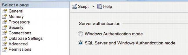
Figure 8-3. Enable SQL Authentication mode

Click OK to dismiss the dialog box. Then open a New Query window, and select master as the destination database. Since Resource Governor settings are applied to all logins, they are configured in the master database.

Next, create a new login for the VIP users:

In a live environment, you would also need to create an associated user and to assign role membership and permissions, and so on. However, for the purpose of this example, you can skip those steps.

Resource Governor includes two standard resource pools: DEFAULT and INTERNAL. All connections are assigned to the DEFAULT pool, and functions such as the lazy writer, checkpoint, and ghost record cleanup are assigned to the INTERNAL pool. Both pools have a minimum and maximum CPU and memory set to 0 percent and 100 percent, which means they effectively aren’t constrained. You can modify the settings of the DEFAULT pool, but not the INTERNAL pool.

You would like to guarantee your VIP users a significant fraction of available CPU time, so you need a new RESOURCE POOL:

This says that for the group of connections assigned to this pool, Resource Governor will guarantee a minimum of 80 percent of the CPU, and the pool can use up to 100 percent. However, those allocations apply only when CPU uses becomes constrained. If VipPool is using only 5 percent of the CPU and DEFAULT connections are using 85 percent, then CPU use is unconstrained, and Resource Governor won’t change the way CPU time is allocated. However, if connections assigned to the VipPool wanted to increase their usage to 50 percent, then Resource Governor would step in and reduce CPU use by the DEFAULT pool from 85 percent to 50 percent so that both pools could operate within their specified parameters.

The sum of all minimum allocations can’t exceed 100 percent.

Resource allocation works similarly with the maximum parameters. The resources used by each pool can exceed their specified maximums, as long as there isn’t any contention. Resource Governor never limits the total CPU used by SQL Server; it only adjusts the allocations of CPU use to particular pools or groups. If a pool had a maximum allocation of 50 percent CPU and no other pools were active, it would be able to use 100 percent of the CPU if it needed to do so.

Next, create a resource WORKLOAD GROUP, and assign it to the resource pool:

You can have multiple groups in the same pool. Each group can have a different priority within the pool. You can also set limits for each group on things like the maximum CPU time that can be used by a single request or the maximum degree of parallelism.

Next, create a classifier function in the master database. Double-check that your query window in SSMS is set to the master database first (or execute USE master):

If the current login is vip, then the function returns VipGroup, which is the name of the WORKLOAD GROUP to which the connection will be assigned.

The classifier function can look at any system parameters you like to determine to which WORKLOAD GROUP the current connection belongs. You return the group name as a SYSNAME (a string). Since the classifier function runs for every login, it should execute quickly to avoid performance issues.

The previous function determines group membership based on the current login name. You might also look at things like the application name, using the APP_NAME() function (you can set its value in your connection string with Application Name), the user’s role, the time of day, and so on.

Next, assign the classifier function to Resource Governor:

Finally, activate the changes:

One handy aspect of Resource Governor is that you can change the resource allocations on the fly, while the server is running. If the usage patterns on your system differ significantly at different times of the day, week, or month, you might run a SQL Agent job to configure Resource Governor appropriately for those times.

If you change the classifier function, keep in mind that connections are assigned to a WORKLOAD GROUP only when they are first created. An existing connection would have to be closed and then reopened in order to use a new classifier function. With standard connection pooling on ASP.NET, that may not happen as soon you might expect.

SSMS also provides a GUI that you can use to manage Resource Governor. To see the changes you just made, open Management in Object Explorer. Then right-click Resource Governor and select Properties. SSMS will display a dialog box similar to the one in Figure 8-4.

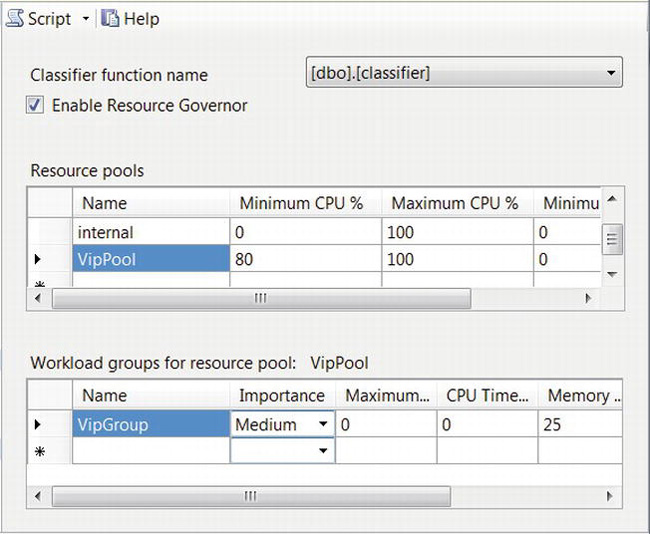
Figure 8-4. Resource Governor management GUI in SQL Management Studio

Testing

To test the changes, open a new instance of SSMS, but connect to SQL Server using the vip login and password that you created rather than your usual credentials. Put the following code in both the original window and the new one:

This is a CPU-bound script that just increments a counter as much as it can over a 30-second period. Start the script in the original window, and then as quickly as you can afterward, start it in the vip window so that both windows are running at the same time.

When the commands complete, you should see that the final count in the vip window is roughly 80 percent of the sum of the two counts. On my local machine, it was about 78 percent, rather than the 50 percent or so that it would be without Resource Governor.

To use this feature from ASP.NET, your code should use different connection strings depending on the nature of the command to be executed, and the type of user who will be requesting the command. For example, anonymous users, logged-in users, VIP users, and logging might all use connection strings with differences that you can identify in your classifier function, such as login name or application name, as described earlier.

Scaling Up vs. Scaling Out

As database servers approach their capacity, one way to grow is to scale up by increasing the capacity of your existing servers. The other way is to scale out by adding additional servers. Each approach has its pros and cons.

Scaling Up

In general, scaling up to add capacity to your site is easier and more cost effective, from both a hardware and a software perspective, than scaling out. However, you will of course reach a limit at some point, where you can’t scale up any more. At that point, scaling out becomes your only alternative.

There are also cases where you want to improve performance, rather than to add capacity. In that event, there are times where scaling out is more effective than scaling up.

In deciding which way to go, one of the first things to look at is how busy the CPUs are. If they’re close to 100 percent most of the time, then you’re CPU bound, and adding more I/O capacity or more memory won’t help. You can add more CPU sockets or cores, or switch to CPUs with a larger cache or a higher clock rate. Once your system has reached its capacity in those areas, you will need to upgrade the entire server to continue scaling up. The associated cost factor is often a good motivator for scaling out at that point instead. However, in my experience, there is usually plenty of room for improvement in other areas before you reach this point.

For I/O-bound systems, a common scenario would be to scale up by adding more memory first, up to your system’s maximum (or approximately the size of your database, whichever is less) or what your budget allows. Next, add more disks and/or controllers to increase your system’s I/O throughput. I/O bound servers can often benefit from a surprisingly large number of drives. Proper disk subsystem design is critical and has a huge impact on performance. See Chapter 10 for additional details.

In the process of architecting a scaling approach, there are a couple of things to keep in mind:

• Adding more I/O capacity in the form of a new server (scale out) is more expensive than adding it to an existing one (scale up).
• You can increase database write performance by first making sure that your database log files are on dedicated volumes and then by adding more drives to those volumes. That’s much less expensive than adding more servers.
• Adding I/O capacity won’t help if your system is CPU bound.

Scaling Out

When you reach the point where scaling out makes sense, you can partition your data in several different ways:

• Horizontally: Place parts of your tables on each server. For example, put users with names starting from A to M on server #1, and put users with names starting from N to Z on server #2. For the boundaries to be adjustable, you may also need some new “directory” tables, so your application can tell which servers have which rows.
• Vertically: Place entire tables on one server or another. Ideally, group the tables so that the ones that participate in SQL joins with each other are on the same server.
• Read-only servers: You can place your read-only data onto separate servers. The easiest approach would be to copy all the related tables, rather than trying to divide them in some way. You can keep the machines with read-only copies in sync with a writable copy by using replication and load balance several together for additional scalability, as in Figure 8-5. You can configure the servers as a scalable shared database, with a common data store, or as separate servers, each with its own data.

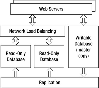
Figure 8-5. Load-balanced read-only databases kept in sync with replication.

• Write-mostly servers: If your application does a lot of logging, or other heavy writes, you can partition that work off onto one or more servers dedicated to that purpose. However, as I mentioned, increasing the write performance of an existing server is usually less expensive than using multiple new servers.

If your database contains large amounts of read-only data, you may be able to improve performance by moving it onto a read-only filegroup. That allows SQL Server to make several optimizations, such as eliminating all locks.

Another design parameter is the possibility of using SQL Express. For example, the load-balanced array of read-only servers shown in Figure 8-5 could be running SQL Express. That can be particularly effective if the database is small enough to fit in memory so that I/O isn’t an issue. However, if I/O is an issue, it’s better to create a single scaled-up server that’s faster and less expensive than an array of cheap servers.

Identifying System Bottlenecks

To determine which type of scaling would be most effective, you can use Windows performance counters to help identify your system’s bottlenecks. You can configure and view performance counters using the perfmon tool. There are a staggering number of counters from which to choose. The ones I’ve found to be most useful for SQL Server scalability analysis are included in the following list. Ideally, you should make all measurements when your database is under peak load and after the database cache is fully warmed up and populated.

• PhysicalDisk, for all active volumes used by the database:
  • Avg. Disk Queue Length: For OLTP systems, this should be less than one per active spindle (not including the extra drives needed for your RAID configuration). For example, if you have 20 spindles in RAID 10, that would be 10 active spindles, so the counter value should be less than 10. For staging databases, the value can be as high as 15 to 20 per active spindle.
  • Avg. Disk sec/Transfer: Your target should be under 0.020 (20 ms) for reads, and under 0.005 (5 ms) for writes to the database log.
  • Disk Transfers/sec: A properly configured data volume using 15,000 rpm drives on a quality hardware RAID controller or SAN should be capable of roughly 400 transfers per second per active spindle. A log volume with the same type of drives should be able to do 12,500 transfers per second per active spindle.
• Processor
  • % Processor Time: The average use should be below about 75 percent. Brief peaks to 100 percent do not necessarily indicate that your system is underpowered. Since this counter shows the average use over all CPU cores, you should also check Task Manager to make sure you don’t have a single process that’s consuming all or most of one or more cores.
• SQLServer:Buffer Manager.
  • Buffer cache hit ratio: This shows how often the data you request is already in memory. If this is below 90 percent, you may benefit from additional memory. Ideal values are above 99 percent.
  • Lazy writes/sec: This shows how often the lazy writer thread is writing dirty pages to disk. Values greater than 20 indicate that more memory could help performance.
  • Page life expectancy: This indicates how long pages are staying in cache, in seconds. Values less than about 350 would be one of the strongest indications that you need more memory.
• SQLServer:Memory Manager.
  • Target Server Memory (KB): This indicates how much memory is available for SQL Server.
  • Total Server Memory (KB): This indicates how much memory SQL Server is currently using. If Total Memory is well under Target Memory, that’s an indication that you probably have enough memory. However, you shouldn’t use these counters to determine whether you don’t have enough memory. In particular, if they’re equal or close to equal, that by itself does not mean that you need more memory.

I often prefer to use the report format in perfmon, as in Figure 8-6. You can select report format from the Change Graph Type button at the top of the panel.

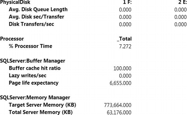
Figure 8-6. SQL Server performance counters in perfmon’s report format

High Availability

Load-balanced web servers provide resilience against hardware failures at the web tier. High availability technologies such as database clustering and mirroring can provide a similar type of resilience for your database tier.

There are a few important performance-related trade-offs between clustering and mirroring. With clustering, there is very little additional overhead during normal operations. However, if a failure happens, it can take 30 seconds or more for the backup server to come online. Any transactions that were in progress at the time of the failure will have to be rolled back. In addition, the backup server will start with an empty RAM cache, so performance will probably be poor for a while after the switchover, until the cache fills.

With mirroring, the active and backup servers are both always running, so switchover takes only a couple of seconds. However, the trade-off is a slight degradation in performance during normal operation, since the active database has to forward all data modification commands to the backup server. You can minimize the impact of that additional overhead by using asynchronous mirroring. When the backup server comes online, its RAM cache may not be identical to that of the primary server, but it won’t be empty either, so the post-switchover performance loss shouldn’t be as significant as with a cluster, assuming that the hardware of both mirrors is the same.

Another trade-off between clusters and mirrors is that you can place read-only queries against a mirror but not against the backup server in a cluster. The hardware you use for mirrors can be anything that will run SQL Server; the servers don’t even have to be identical (although it’s a good idea if they are).

With clustering, you should only use hardware that Microsoft has specifically approved for use in a cluster. Clusters require a multiported disk subsystem, so both the primary server and the backup can access them. Mirrors can use standard single-ported disk controllers. Clusters tend to be more complex to configure and maintain than mirrors.

You can geographically separate the machines in a mirror. You should keep machines in a cluster physically close to each other, ideally in the same rack.

Although SQL Standard supports only two-node clusters, with SQL Enterprise you can have up to 16 nodes. In a multi-database-server environment, that means you should need fewer standby (and idle) machines. For example, you might have three active nodes and one standby node, configured so that any of the active machines can failover to the standby.

A so-called active-active configuration is also possible. For example, you might have three active nodes, where each node can fail over to another active node. However, if your servers regularly operate at close to capacity, that configuration can result in one node becoming overloaded in the event of a failure. Having an idle standby node allows much more resilience in the event of a failure.

Miscellaneous Performance Tips

Here are a couple of additional performance tips:

• Database connections are pooled by default by ASP.NET. To minimize the number of simultaneous connections your application needs, you should open a connection right before you use it and then call Dispose() as soon as you’re done (ideally with a using statement).
• Keeping the connection open longer is acceptable, provided that the total execution time can be reduced by using a transaction, command batching, or multiple result sets.
• Minimize filesystem fragmentation and the resulting reduction in disk throughput by setting a large initial file size for your database and log, as well as a large incremental size. Ideally, the file sizes should be large enough that neither the data file nor the log should ever have to grow.
• To minimize fragmentation that might be introduced by the NTFS filesystem, ideally each disk volume should only hold one database data or log file.
• Don’t shrink or autoshrink your files, since that can undo the benefits of giving them a large-enough-to-grow size.
• Minimize the number of databases you have. Using multiple databases increases maintenance and deployment effort and complexity and can cost you performance. More than one database log file means that you either need multiple dedicated drives to ensure that all writes will be sequential or need to combine multiple logs on a single drive and therefore lose the ability to do sequential writes (with an associated performance hit). You can achieve all of the partitioning and security benefits of multiple databases with just one instead.
• Consider using SQL CLR for stored procedures or functions that contain a large amount of procedural code. T-SQL is great for set-based operations, but its procedural features are minimal. As with vanilla stored procedures, avoid putting too much business logic in a SQL CLR procedure. However, if a little extra logic in the database can help you avoid some round-trips, then it’s worth considering. SQL CLR is also a great way to share constants between your web application and your stored procedures.
• Avoid aggregation queries as much as you can. When you need them, consider caching their results on the web tier or in a small table, which you then recompute periodically. That way, you can easily share the results among multiple web servers, further minimizing the number of times you need to run the queries. Each web server can use SqlCacheDependency to watch for changes in the results table. Another option is to use Analysis Services to generate preaggregated results and to make your aggregation queries against that data instead of against the relational store. I’ll cover that approach in detail in the next chapter.

Summary

In this chapter, I covered the following:

• How SQL Server can act like a large cache if it has enough RAM and how using the 64-bit version is an important part of being able to use that memory effectively.
• The importance of placing database log files on a volume by themselves.
• Using stored procedures instead of dynamic SQL whenever you can.
• Using command batching, table-valued parameters, and multiple result sets to improve performance by reducing the number of database round-trips.
• Using transactions to reduce I/O pressure to the database log, which can significantly improve database write performance.
• Improving the performance of future queries with data precaching. By executing a similar query before the anticipated one, you can read the required data pages into memory before they are needed.
• Using clustered and nonclustered indexes to speed up your queries.
• Choosing indexes to minimize table and index fragmentation.
• Constructing and using efficient data paging queries.
• Integrating data paging with a GridView control, an ObjectDataSource, per-request caching, multiple result sets, and ControlState.
• Choosing ADO.NET over LINQ or the Entity Framework when you need top performance.
• Using the XML data type, querying and modifying XML columns, and using XML indexes and schemas to improve query performance.
• Partitioning large tables to improve performance and ease maintenance tasks.
• Using full-text search to improve query performance.
• Using Service Broker to move or defer long-running tasks.
• Subscribing to and using data change notifications.
• Using Resource Governor to balance or give priority to workloads on busy servers.
• Choosing between scaling up and scaling out and knowing whether your server needs more RAM, disk, or CPU.
• The performance-related trade-offs between using clustering or mirroring for high-availability.