8

Lift and Wings in 3D at Subsonic Speeds

In this chapter, we extend the discussion of lift from 2D to 3D take up the topics of the flow around a 3D wing, the lift distribution on a 3D wing, the induced drag, wingtip devices, and the manifestations of lift in the extended flowfield. Finally, we'll delve into some of the interesting issues that arise when wings are swept.

8.1 The Flowfield around a 3D Wing

The flow around a 3D wing must differ in some basic ways from the flow around a 2D airfoil, simply because of the finite span and the resulting flow gradients in the spanwise direction. In this section, we'll first describe the general features of 3D wing flowfields, and then we'll look at how they can be explained. The classical approach (starting with the early work of Prandtl and others, see historical sketch by Giacomelli and Pistolisi, in Durand, 1967a) looks at the distribution of bound vorticity and the vorticity in the wake and deduces the velocity field everywhere else using the Biot-Savart law. Though this yields correct results if the correct vorticity distribution is used, it is not a real physical explanation in the cause-and-effect sense, as we argued in Sections 3.3.9 and 7.2. So we'll also seek an explanation based on the local balance of force and acceleration, that is, the interaction of the pressure and velocity fields. We constructed explanations of this type for the generic flow around an obstacle in Section 5.1 and the flow around a 2D lifting airfoil in Section 7.3.3. Even in those relatively simple flow situations, however, we found that qualitative arguments alone did not enable us to predict the flow a priori. Instead, we had to settle for explaining things “after the fact,” based on prior knowledge of what the pressure and velocity fields look like. In the case of a 3D wing, we will also have to rely heavily on prior knowledge of the flow structure.

8.1.1 General Characteristics of the Velocity Field

The flow around a 3D wing is similar in some ways to the flow around a 2D airfoil, so to start the discussion, let's review the relevant features of the flow in the 2D case. In the flow over a lifting 2D airfoil, the velocity disturbances produced by the airfoil die out rapidly in all directions, including downstream. Downstream of the airfoil, the only significant velocity “signature” of the lift production is the downwash field, which carries a flux of downward momentum across any vertical plane, corresponding to half of the lift. With increasing distance downstream, this downwash spreads out rapidly in the vertical direction and becomes very diffuse, but the flux of downward momentum remains constant. As we discussed near the end of Section 7.3.4, the flow around a 2D airfoil in the inviscid case is reversible, in that an onset flow that is uniform in the limit far upstream becomes uniform again in the limit far downstream, and the same flow pattern and pressures would arise if the flow were run in the reverse direction. In a viscous flow in the attached-flow regime, the flow outside the boundary layer and wake still follows the reversible pattern quite closely. In addition to the near-reversibility of the general flow pattern, there is also very little permanent vertical displacement of streamlines between upstream and downstream (none in the inviscid, shock-free case). And, of course, all these flow features are by definition uniform in the spanwise direction.

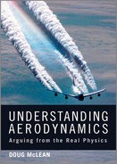
Now consider a 3D wing of finite span, with moderate-to-high aspect ratio, operating in the attached-flow regime. At any station along the span of the wing other than very close to the tips, the chordwise distributions of pressure and boundary-layer development are not much different from those of a 2D flow, and the streamlines projected in a longitudinal plane look qualitatively like the flow around a 2D airfoil, as illustrated in Figure 8.1.1. But this projected view misses an important aspect of the 3D flow; that is, that the streamlines of the 3D flow don't generally lie in planes as those of a 2D flow do. A key part of what distinguishes the 3D flow from the flow around a 2D airfoil is a significant out-of-plane component to the motion. This out-of-plane component would be difficult to discern if it was shown in a perspective view like Figure 8.1.1, but it is important nonetheless.

We can visualize the 3D flowfield more clearly in terms of velocities projected in planes perpendicular to the freestream, as illustrated in Figure 8.1.2. This cross-stream velocity field develops in conjunction with a pressure field that is nonuniform in the spanwise direction. The general pattern is characterized by downward flow in the area between the wingtips, upward flow outboard of the tips, outboard flow below the wing, and inboard flow above the wing. Note that these lift-induced velocities are not concentrated closely just around the wing itself or the wingtips, but are spread fairly diffusely over a wide area of the flowfield.

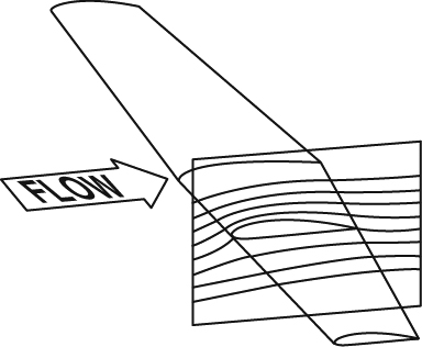
Figure 8.1.1 Flow around a 3D wing viewed in terms of streamlines projected in a plane perpendicular to the span is similar to flow around a 2D airfoil

Figure 8.1.2 Flowfield around a lifting wing illustrated by velocity vectors in a cross-flow plane. This general flow pattern is well established around the wing itself and persists for long distances downstream

The streamwise development of the cross-stream velocity field in the 3D flow is quite different from anything in the development of a 2D airfoil flow. In the flow more than about one wingspan ahead of the wing, the velocity disturbances are small and are distributed diffusely, as they are in the 2D case. As we approach closer to the wing, a pronounced upwash appears ahead of the leading edge, as in the 2D case. As we pass behind the leading edge and over the wing itself, the general flow pattern shown in Figure 8.1.2 becomes well established. Behind the wing, the flow pattern continues to evolve, with velocities increasing in parts of the field and decreasing in others, but continuing to look qualitatively like Figure 8.1.2. At a distance on the order of a wingspan behind the wing, the flow will have settled into an asymptotic pattern, and then it changes only very slowly over long distances downstream. This is a key distinction between 3D and 2D: While the velocity disturbances in the 2D case begin to decrease immediately behind the airfoil and become very small and very diffuse far downstream, the cross-stream velocity field that develops in 3D persists for very long distances downstream. Another way to look at this distinction is in terms of reversibility: Both the 2D and 3D cases start with a uniform onset flow upstream, but while the 2D flow becomes uniform again downstream, the 3D flow becomes nonuniform, with persistent transverse velocities even at very large distances downstream. It is therefore not even close to being reversible like the flow around a 2D airfoil.

At the location of the wing itself, we have a well-established flow pattern in which the wing is flying through air that is already moving generally downward between the wingtips. Thus the wing can be thought of as flying in a downdraft, or downwash, of its own making. At the location of the wing itself, the downwash can in general vary considerably, both spanwise and chordwise. But on a high-aspect-ratio wing, we can simplify the picture: We can think of the downwash at the location of the wing as consisting of two parts, a 2D part that would be there if the local airfoil section were in a 2D flow at the same sectional lift (not the same geometric angle of attack), and a 3D part that is a result of finite span. In the limit of high aspect ratio, the 3D part of the downwash is constant along the chord at a given span station. The 3D downwash can thus be seen as a downward shift in the apparent angle of attack of each airfoil section along the wing, often called the induced angle of attack. For positive total lift, the effect of the induced angle of attack, integrated over the span, always corresponds to a reduction in the apparent angle of attack of the wing.

One consequence of the apparent downdraft in which the wing is flying is that a 3D wing generally requires a higher geometric angle of attack to achieve the same lift coefficient as a corresponding 2D airfoil, a fact we'll make use of when we attempt to explain features of the 3D flowfield. And because the downwash increases with angle of attack and thus subtracts progressively more from the lift, the lift slope of a 3D wing is generally less than that of a 2D airfoil section.

The other important result of the downwash is that the total apparent lift vector is tilted backward slightly. This backward component of the apparent lift is called induced drag, and the work done against it is reflected in the kinetic energy of the large-scale flow pattern. We'll discuss the physics and the theory of induced drag further in Section 8.3.

In Figure 8.1.2, we saw that the spanwise velocity components behind the wing are in the outboard direction below the wing and in the inboard direction above the wing. There is thus a mismatch, or jump, in the spanwise velocity, and this jump constitutes a vortex sheet that is shed from the trailing edge and convected downstream. The development of this vortex wake is our next topic. The induced drag and the presence of vorticity that is convected downstream are both earmarks of the general irreversibility of the 3D flow pattern.

8.1.2 The Vortex Wake

The trailing vortex wake is a distinctive feature of the lift-induced flowfield, and it plays a prominent role in discussions of induced drag and in the quantitative theory. The nature of the vortex wake and its role in induced drag have been a source of some serious misunderstandings, so we'll take extra care in the following discussion to point out the common misconceptions, to help ensure that we develop a correct understanding.

As we noted above, the vortex wake starts as a vortex sheet shed from the trailing edge of the wing as a byproduct of the establishment of the flow pattern shown in Figure 8.1.2. It is a necessary part of the flowfield because the wing cannot produce the general flow pattern of Figure 8.1.2 without also producing the jump in spanwise velocity between the streams that pass above and below the wing. Even if we model the flow around the wing as inviscid, a vortex sheet must be shed if the lift is nonzero. Milne-Thomson (1966, Section 3.31) describes the shedding of a vortex sheet from a body in 3D inviscid flow as the “bringing together of layers of air which were previously separated, and which are moving with different velocities.” Of course, if a shed vortex sheet is wetted on both sides by air that has come from the freestream without any change in stagnation pressure or stagnation temperature, the velocity magnitude on both sides must be the same. So by “different velocities” Milne-Thomson means different flow directions. Farther along in the discussion, we'll attempt to explain how those different flow directions arise in the case of a lifting 3D wing.

Milne-Thomson's quote above provides interesting food for thought and merits a little digression. He's given us an intuitively appealing way to think of what's happening when the vortex sheet leaves the trailing edge, but “previously separated” in this context is ambiguous. If all it means is that the layers of air were not together prior to being joined, then there's no problem. But it could also be taken to imply that the layers of air coming together at the trailing edge were separated from each other at some location upstream, presumably where they attached to the wing at the attachment line. This more specific meaning wouldn't be precisely correct. On a wing of finite span, a layer of air can come only very close to attaching to the surface, but can't actually attach in a rigorous sense. Recall from our discussion in Section 5.2.2 that a finite attachment line is at best a band of approximate attachment, and that only discrete filaments of flow can actually attach to the surface at singular points. Often there is only one point of attachment, like the nodal point marked “N” on the nose of the fuselage of the simple wing-body combination sketched in Figure 5.2.4. In this case, strictly speaking, the layers of air that join at the trailing edge originated from the filament that attached at the nose of the fuselage, not from layers that were split apart by the wing. At any short distance above and below the trailing edge, however, we find layers of air that were similarly close together when they passed near the leading edge. When such layers come close to “joining” at the trailing edge, they generally will have experienced considerable spanwise displacement relative to each other, in addition to the longitudinal displacement that we discussed in connection with 2D flow in Section 7.3.1.

And now to return to our main topic. We've seen that the vortex wake starts its life as a free vortex sheet that seems to originate from the trailing edge of the wing. But the trailing edge cannot be the actual origin of the vorticity in the wake. Because vortex lines cannot end at a solid surface with a no-slip condition (except at singular points of attachment or separation, as we saw in Section 3.3.7), the vorticity in the wake must originate in the viscous or turbulent boundary layers on the upper and lower surfaces of the wing. Where does this lead? If we look at all of the vorticity present in the 3D flow in the boundary layers and the wake, we see a very complicated picture, but it can be simplified greatly if we boil it down to its essentials. With regard to the global flowfield, what really matters is the net vorticity at any station on the wing or wake, as seen in a local plan view. At a station on the wing planform, the net vorticity would thus be defined by integration through both the upper and lower surface boundary layers; and at a station on the wake, it would be defined by integration through the entire viscous layer. The complicated distribution of vorticity through the viscous layer at a given station is thus replaced by a single vector value that is much easier to visualize.

Viewed thusly in terms of net vorticity, the shed vortex sheet is actually a continuation of the bound vorticity associated with the lift of the wing, which we discussed in Section 7.2 in connection with lift in 2D. This view in terms of net vorticity was option 3 of the ways of looking at bound vorticity that we identified in that discussion, illustrated in Figure 7.2.1c. In the 3D case, as the lift per unit span decreases in the outboard direction along the span, the circulation and total bound vorticity flux must also decrease. The vorticity representing this loss in total strength cannot just disappear and is shed from the trailing edge into the flowfield, supplying the vorticity that forms the vortex wake.

Now imagine the net vorticity on the wing and in the wake as an array of vortex filaments. These filaments take on a general horseshoe shape, as shown in Figure 8.1.3. Since each filament of this system forms a horseshoe, if we take a cut through the wake anywhere downstream of the wing, at the plane marked A, for example, the filament will be cut in two places, and the flux of vorticity passing through the cut will be equal and opposite in the two places. (Recall from Section 3.3.7 that a vortex filament is a construct that carries the same flux of vorticity along its entire length.) Thus it is clear from the horseshoe configuration of the vortex system that the total vorticity flux passing through a cut through the whole wake is zero. We could arrive at the same conclusion by placing a closed contour in the cut such that it encloses the entire wake, and invoking Stokes's theorem on a capping surface that bulges out ahead of the wing and thus cuts none of the vorticity. The circulation around the closed contour must then be zero, and there can then be no net vorticity flux through any cut across the entire wake.

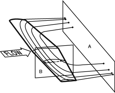
Figure 8.1.3 Bound and trailing vorticity of a lifting wing viewed as vortex filaments. The plane marked “A” illustrates how these filaments would be cut by a transverse plane behind the wing, and the plane marked “B” illustrates how they would be cut by a longitudinal plane through the wing

Another conclusion that follows from the horseshoe configuration of the system is that if we take a cut through the wing anywhere along the span, at the plane marked B in Figure 8.1.3, for example, the total fluxes of vorticity shed from the trailing edge on opposite sides of the cut will be equal and opposite, and their magnitudes will equal the flux of bound vorticity at that span station. Then, as a special case, we can say that when the lift distribution is laterally symmetrical, the total vorticity flux of the sheet shed from each side must equal the flux of bound vorticity at the center.

Like the boundary layers in which it originated, the wake shear layer is a real physical shear layer filled with small-scale turbulent motions. The idealized inviscid theories model the shed vortex wake as a thin vortex sheet of the kind we discussed in Sections 3.3.7 and 3.3.8, and illustrations often show it that way for simplicity. In all of the discussion that follows, “vortex sheet” can be thought of as referring to either a real physical shear layer or to an idealized thin sheet.

The development of the vortex sheet after it leaves the trailing edge is illustrated in Figure 8.1.4. The vortex lines in the sheet leave the trailing edge and follow the general direction of the flow downstream. In the case of the ideal thin vortex sheet, the vortex lines are aligned with the mean of the velocity vectors above and below the sheet, as in Figure 3.3.8c. Within the first couple of wingspans downstream, the sheet generally rolls up toward its outer edges to form two distinct vortex cores. (This is the general pattern for a wing in the “clean” condition, flaps up. The flaps-down pattern is more complicated, with cores forming behind flap edges as well behind the wingtips.) Although the vortex cores are distinct, they are not as concentrated as they are sometimes portrayed, because a considerable amount of air that was initially nonvortical is entrained between the “coils” of the spiral formed by the sheet during rollup.

Figure 8.1.4 Development of the vortex wake downstream of a lifting wing. The lines drawn on the sheet are the vortex lines of a continuous distribution of vorticity in the sheet

In simplified theoretical models, such as the Trefftz-plane theory we'll discuss in the next section, the vortex lines are assumed to stream straight back from the trailing edge in the direction of the freestream, and the deformation and rollup of the wake are not represented. The classic argument is that the assumption of a nondistorting wake is valid in the limit of zero lift on the wing. For finite lift, however, it is kinematically impossible for the wake sheet to remain undistorted. Obviously a nonuniform downwash field behind the wing will distort the wake, and downwash fields behind lifting wings are generally nonuniform. Even in the case of an elliptic spanwise load distribution, which we'll see in the next section ideally produces a uniform downwash “contribution” from the trailing vortex wake, the “contribution” from the bound vortex is nonuniform, and the sheet must still distort and ultimately roll up. Even if we could find a situation in which the downwash was uniform, however, it would still be impossible for the wake to remain undistorted. This is sometimes attributed to an “instability” (Milne-Thomson, 1966, for example, in Section 10.4 refers to the wake sheet as “unstable” but does not provide a detailed explanation, and in Section 3.31 hints that viscosity might play a role). Spalart (1998), however, has shown that it is not an instability, but a result of the basic kinematics of the sheet, associated with the singularity in its strength at the edge, due to the usual infinite slope of the loading at the tip. In the real world, of course, there is no singularity, but there still tends to be a high concentration of vortex strength, and real wake sheets still roll up at their edges.

Note in Figure 8.1.4 that in the early phase of wake rollup, the vortex lines are swept outboard toward the rolling-up edges of the vortex sheet. As the sheet rolls up into coils, the vortex lines become helical, and when rollup is complete, the vortex lines in the outer part of the core appear as illustrated in Figure 8.1.5. In the idealized inviscid world, however, the vortex cores would appear as tightly wound spirals, continually stretching and tightening. In the real world, the coils of the spiral merge by turbulent diffusion, and diffuse vortical cores are formed in which the vortex lines are still helical. The helical vortex lines are very closely aligned with the helical streamlines. This is consistent with Crocco's theorem (Equation 3.8.8) and with the fact that the total-pressure loss associated with the viscous drag has diffused throughout the wake, so that the local total-pressure deficit is relatively small.

Figure 8.1.5 Helical vortex lines and the associated velocities in the rolled-up vortex cores. The helical vortex lines line up closely with the helical streamlines

To get an idea of how the vorticity should be distributed within the cores, consider the initial distribution of vortex strength in the sheet that leaves the trailing edge and is eventually “wound up” into the cores. Figure 8.1.6 illustrates the distributions of bound and shed vorticity for a typical wing, showing that the shed vorticity is most intense at the tips and is much weaker inboard. Based on this, we should expect intense vorticity in the center of the rolled-up core and much weaker vorticity in the outer part.

Now let's look at the details of the velocity field in the mature wake far from the wing. The first feature we must note is that the pair of vortex cores descends slowly relative to the flight path of the airplane. This is often attributed to “mutual induction,” but it is better to think of it simply as convection by the downwash behind the wing, which persists far downstream because there is practically nothing acting to stop it. We'll consider the cause-and-effect issues further in Section 8.1.4. As the cores descend, they carry with them a “descending oval” of fluid, as illustrated in Figure 8.1.7.

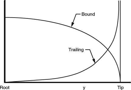
Figure 8.1.6 Sketch of typical distributions of the fluxes of bound and shed (trailing) vorticity, showing that shed vorticity is heavily concentrated near the tip

Figure 8.1.7 Sketch of the descending “oval” associated with the mature, rolled-up vortex wake, in terms of streamlines in the reference frame descending with the oval

The flow within much of the vortex core in each half of the descending oval is nearly axisymmetric. Figure 8.1.8 shows how the vertical velocity, the vorticity, and the pressure are distributed spanwise along a horizontal line through the centers of the cores (based on rollup calculations by Spalart and consistent with measurements by Widnall; see Spalart, 1998). Only the right half of the field is shown, with a symmetry plane assumed at y/b_o = 0. For comparison, dashed curves show what these distributions would be if all of the vorticity were concentrated in a pair of line vortices, and the flow everywhere else were irrotational (potential flow). Another dashed line shows what the distributions would look like for a Rankine core, with the core in solid-body rotation with constant vorticity, a model we'll look at again in Section 8.3.3 in connection with induced drag.

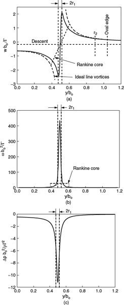
Figure 8.1.8 Details of the flow field of the mature vortex wake, shown as distributions along a horizontal cut through the middle of the descending oval. (a) Vertical velocity w. (After Spalart (1998).) (b) Vorticity, estimated from w, assuming axisymmetric flow in core. (c) Pressure, estimated from w, assuming axisymmetric flow in core. (From Spalart, 1998)

In the real flow (solid curves), the peak circumferential velocity (Figure 8.1.8a) is quite high and occurs at a small radius r₁ from the center of the core. Significant vorticity persists out to a much larger radius r₂, which extends almost to the center plane and to the boundary of the oval. This persistence of the vorticity is clearly seen in the fact that the velocity profile does not fair in to the potential-flow curve until it reaches r₂, but it is hard to see in the plot of the vorticity distribution (Figure 8.1.8b) because the scale was chosen to show the very high vorticity at the center of the core. The intense vorticity concentrated in the central peak and the lower levels in the rest of the core are consistent with the vorticity distribution in the initial sheet that feeds the core, as we expected from our earlier discussion. The plot of the pressure distribution (Figure 8.1.8c) shows that very low pressures are concentrated only in the intense central core.

The low pressure in a vortex core is accompanied by low temperature, which often causes condensation of water vapor, making the core visible. How much of the core is visible under such conditions depends on the situation. In a newly forming core just downstream of a wingtip or flap end, usually only a central portion of the core is marked by condensation, making the core appear more compact than it really is. In the farfield, the situation is more complicated. Often, engine exhaust has been rolled up into the cores, carrying with it water vapor and condensation nuclei (soot) from the engines into the outer parts of the cores. Under such conditions, nearly the entire turbulent wake of the airplane may be visible. But the picture can change over time, as the condensation evaporates, as it appears to be doing in the photos in Figure 8.1.10.

The vortex cores are often referred to as “wingtip vortices,” though we can see from the foregoing that this is a bit of a misnomer. While it is true that the cores line up not very far inboard of the wingtips, the term “wingtip vortices” implies that the wingtips are the sources of all of the vorticity. Actually, as we saw in Figure 8.1.4, the vorticity that feeds into the cores generally comes from the entire span of the trailing edge, not just from the wingtips. Though it is difficult to tell from the curve in Figure 8.1.8b, the concentrated peak of high vorticity inside of r₁ in Figure 8.1.8b accounts for only about 30% of the total vorticity in the core.

Figure 8.1.9 illustrates another feature of the velocity field associated with the rolled-up wake. In the direction parallel to the core axes, there is usually an axial “jet” in the downstream direction, away from the wing.

The decay of the trailing vortex cores, if it were by viscosity alone, would be extremely slow, and even though the cores are turbulent at all but the lowest Reynolds numbers, turbulent transport is suppressed by flow curvature, and the decay of the vortices is still very slow. At the scale of a large airplane, the vortices would persist for hundreds of miles behind the wing if viscosity and small-scale turbulent diffusion were the only dissipation mechanisms. In actuality, the vortices typically persist for something more on the order of 10 miles, and the eventual breakup of the wake is not by small-scale turbulence but by large-scale motions and distortions of the vortices, resulting from slow-growing instabilities such as the Crow instability (Crow, 1970). Figure 8.1.10 shows a progression of breakup initiated by the Crow instability, made visible by water condensation. Spalart (1998) refers to this process as collapse, to contrast it with the much slower process of decay. We'll consider the breakup process further and speculate on what the whole flowfield looks like in a time-averaged sense on a very large scale, in Section 8.5.5.

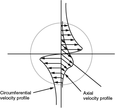
Figure 8.1.9 Sketch of a “jet” of axial velocity in a vortex core

Figure 8.1.10 Progression of vortex breakup initiated by the Crow instability, made visible by condensation. Wake of a B-47 photographed at 15-second intervals. (From Crow, 1970)

8.1.3 The Pressure Field around a 3D Wing

If we take longitudinal vertical cuts through the flowfield as we did to look at streamlines in Figure 8.1.1, but look at the pressure field instead, what we see looks qualitatively like what we saw for a 2D airfoil in Figures 7.3.11 and 7.3.24. This is a view in which 3D effects are difficult to discern. For purposes of understanding the 3D flow, the view in cross-stream planes is more informative. Consider pressure distributions in a succession of cross-stream planes: one a short distance upstream of the wing, one through the middle of the wing, and one immediately downstream of the wing. These are illustrated in Figure 8.1.11 for both the 2D and 3D cases. The cuts shown for the 2D case are just cross-sections of the generic 2D lifting pressure field we considered in Figure 7.3.11. In making these sketches, I've assumed that the maximum chord and load per unit span at the center plane of the 3D wing are the same as for the 2D airfoil, so that the center section of the 3D wing matches the lift coefficient of the 2D airfoil, not the angle of attack. Because of the downwash in the 3D case (which is one of the things we'll be seeking to explain in Section 8.1.4), the 3D wing will need a higher angle of attack than the 2D airfoil, and eventually we'll come back around to seeing this reflected in our explanation of the velocity field.

Now note in Figure 8.1.11 that the pressure distributions in the 3D case show distinct effects of finite span. As the lift decreases outboard of the center section, a combination of the intensity and vertical extent of the pressure distribution must decrease, depending on the planform and lift distribution of the wing. In this case, we show the vertical extent decreasing, as would be the case if the reduction in local lift load were due mostly to a reduction in chord. Note that there is also a kind of “3D relief” effect, in which the pressure disturbances off the surface inboard are “dragged down” closer to the smaller disturbances outboard. As a result, the vertical extent of the pressure distributions in 3D is smaller everywhere along the span, even at the center section, than it is for the 2D airfoil. This more rapid “dying off” of the pressure disturbances away from the wing in 3D is seen at all stations: ahead of the wing, at the wing, and behind the wing.

8.1.4 Explanations for the Flowfield

Now that we have a qualitative description of the flowfield around a 3D lifting wing, we'd like to explain physically how the flow does what it does. One of the main things we'll want to explain is why the velocity disturbance downstream, which dies off rapidly in the case of a 2D airfoil, persists over long distances in the case of a 3D wing. As we've already noted, the classical approach to this is to describe the distribution of the vorticity, both the bound vorticity and the vorticity in the wake, and to use the Biot-Savart law to infer what the velocity field does. Of course the Biot-Savart law is applicable, and all of the features of the cross-flow velocity field near the wing that we saw in Figure 8.1.2 are “explainable” as being “induced” by the bound vorticity and the shed vortex sheet, mostly the part in the near field downstream of the trailing edge. Likewise, the velocity field that persists far downstream, and differs from Figure 8.1.2 only in some details, is consistent with “induction” by the rolled-up vortex wake shown in Figure 8.1.8. An apparent strength of the vorticity-based approach is that the convection of a somewhat compact vortex wake downstream provides an “explanation,” of sorts, for the persistence of the velocity disturbance. A weakness is that the “explanation” that it provides is incomplete in that we had to know or assume a priori how the vorticity is distributed. And we must also remember that even if we know the vorticity distribution, appealing to Biot-Savart only gives a correct description of the flowfield, and that it does not explain it directly in terms of physical cause and effect. The description using Biot-Savart is convenient as a mental crutch and for quantitative purposes, but it is prone to misinterpretation in terms of the induction fallacy, as discussed in Section 3.3.9. The correct view is that the vorticity is not the cause of the flowfield but is more of a passive result of other things that are happening in the flowfield.

Figure 8.1.11 Gross features of pressure distributions in cross-planes in lifting flows. (a) Upstream. (b) Cut through the wing. (c) Downstream

As we noted in the introduction to Section 8.1, a real physical explanation must involve the interaction of the pressure and velocity fields. In the case of a 2D airfoil in Section 7.3.3, the vertical component of the velocity and its interaction with the pressure field played a prominent role in our explanation of the flow. Now let's see how far this kind of thinking can take us in the 3D case, in explaining the cross-flow velocity components illustrated in Figure 8.1.2. Of course, now we'll have to explain the evolution of the spanwise velocity component, in addition to that of the vertical component.

We'll approach the problem by thinking in terms of individual fluid parcels passing through different parts of the pressure field sketched in Figure 8.1.11, and of the pressure gradients the parcels are subjected to during their passage. The most obvious conclusions we can draw have to do with those major portions of the field where one component of the pressure gradient maintains the same sign throughout a parcel's passage through the region. In these situations, the corresponding velocity component is set in motion and not stopped, and we should expect that part of the motion to persist downstream. By inspection of the pressure distributions in Figure 8.1.11, we can see that this mechanism is consistent with the spanwise velocities in the outward direction below the wing and in the inward direction above the wing, and with the upwash outboard of the tips. So these features of the flowfield of Figure 8.1.2, which persist far downstream and have no counterparts in the 2D case, seem to be explainable in terms of simple gross features of the 3D pressure field associated with the lift.

The downwash between the tips is the only major feature of the pre-rollup velocity field not yet explained, and it is more complicated. The vertical component of the pressure gradient, which drives this part of the motion, reverses sign twice for fluid parcels passing above or below the wing, just as it does in the 2D case. In our explanation of the 2D case in Section 7.3.4, we saw that the pressure field participates in a delicate balancing act that results in downwash that decays to zero far downstream of the airfoil. In the 3D case, on the other hand, we know the downwash persists over long distances downstream. With pressure fields that are qualitatively so similar, that is, with two reversals of the gradient in both cases, how do we account for the dramatic difference in the resulting downwash fields? To answer this question, we have to look at the interactions in both cases in more detail.

In the 2D case, there is both upward and downward turning taking place in the flowfield ahead of the airfoil. In connection with Figure 7.3.23, we noted that vertical cuts through the field ahead of the airfoil see the same net flux of vertical momentum across them, corresponding to half the lift, which doesn't change from one cut to another. However, if we limit our attention to a streamtube that passes close to the airfoil above and below, we see that the pressure gradient ahead of the airfoil turns the flow upward, then the gradients above and below the airfoil turn the flow downward, and finally the gradient behind the airfoil turns the flow upward again, canceling the local downwash velocities in an asymptotic sense far away from the airfoil. The upward turnings ahead of the airfoil and behind are just enough to cancel the downward turning that takes place as the flow passes close to the airfoil surfaces.

In the 3D case, the downward turning immediately above and below the wing is stronger than it is in the 2D case, for the same lift. This is because the more rapid dying off of the pressures above and below the airfoil means the vertical pressure gradient near the wing surface is stronger than in 2D. More rapid downward turning, resulting in larger downwash by the time the trailing edge is reached, is also consistent with the fact that the 3D wing requires a higher angle of attack to achieve the same lift. The airfoil pressure field also dies out more rapidly ahead of the airfoil and behind, which results in less upward turning of the flow in those regions. So in the 3D case, we have more downward turning above and below the wing, and less upward turning ahead and behind, with the result that some downwash persists in a central portion of the field behind the wing, that is, between the wake-vortex cores.

To complete this explanation, we must point out that all of these effects of the pressure gradients on the cross-flow velocities constitute only one side of the interaction. Remember that cause-and-effect is a two-way street and that the velocity changes, or accelerations of the flow, are both caused by the pressure gradients and also serve to sustain the pressure gradients. This is the same point that we made a major issue of in our explanation of 2D airfoil flow in Section 7.3.3. There we talked about “confinement” of the “clouds” of high and low pressure and how vertical and longitudinal accelerations of the flow provided that confinement. That description of vertical and longitudinal confinement also applies in the 3D case, but the spanwise component of acceleration also comes into play: The outboard acceleration of the flow beneath the wing and the inboard acceleration above the wing provide spanwise confinement of the pressure differences around a 3D wing.

In the 3D wing flow, the vertical pressure gradients above and below the airfoil are sustained by the downward turning of the flow, just as we noted that they are in 2D. However, a feature of the 3D pressure field that is not so easy to explain in simple qualitative terms is the “3D relief effect” that we described in Section 8.1.3, in which the vertical extent of the pressure distribution in 3D is lower than in 2D for the same chord and lift per unit span. Reducing the vertical extent of the pressure distribution means an increase in the vertical pressure gradient close to the wing surface and a reduction farther from the surface. It is a result of the 3D flow's freedom to accelerate spanwise, but not a simple result to explain.

It is also interesting to note how the pattern of horizontal and vertical velocities that we've just explained fits together in terms of conservation of mass. Referring to Figure 8.1.2, note that the horizontal velocities converge toward the center plane above the wing and diverge from the center plane below the wing. The downwash between the tips thus “exhausts” the converging flow above and “feeds” the diverging flow below. Around the tips, the opposite occurs: divergence above and convergence below, which are “relieved” by the upwash outboard of the tips. So we see that for the horizontal velocities that were set in motion by the wing to persist far downstream, they must be accompanied by downwash between the tips and upwash outboard, and must therefore be part of a general circulatory pattern behind each half of the wing. And, of course, each of these circulatory regions must have vorticity (half of the vortex wake) somewhere inside it.

The final features needing an explanation are the axial jets in the rolled-up vortex cores that we saw in Figure 8.1.9. It has been shown that far downstream of the wing the component of the velocity disturbance parallel to the core axes is nonzero only within the vortical cores (Spalart, 2008). Within the cores, it is clear from Figure 8.1.9 that the axial velocity disturbance is “explainable” as being “induced” by the circumferential component of vorticity associated with the helical configuration of the vortex lines, which, as we've already noted, lines up closely with the helical configuration of the streamlines. A direct physical explanation starts with the observation that balancing the centrifugal forces associated with the circumferential velocities requires a radial pressure gradient, and therefore substantially lower than ambient pressure within the cores, as we saw in Figure 8.1.8c. The air in the cores started at ambient pressure upstream of the wing and, having entered the low-pressure region within the cores, has experienced a net acceleration in the axial direction. And again, our caveat regarding one-way cause and effect applies, and we must remember that the accelerations and the pressure gradients share a mutual interaction.

8.1.5 Vortex Shedding from Edges Other Than the Trailing Edge

So far we've considered the flow over wings of moderate-to-high aspect ratio, assuming that all of the significant vorticity shedding is from the trailing edge. But vorticity shedding is not always confined to trailing edges. On many wings, especially those with squared-off or nearly squared-off tips, the shedding at the tip starts well forward of the trailing edge, on the nearly streamwise “edge” at the tip. In this case, the vorticity can roll up over the wing upper surface, as shown in Figure 8.1.12a. A similar pattern is common on the squared-off outboard edges of deployed trailing-edge flaps. On high-aspect-ratio surfaces, such details near the tips have only small effects on the overall development of the vortex wake and the global flowfield. However, on a low-aspect-ratio wing, shedding from edges other than the trailing edge can dominate the development of the flow. For example, on low-aspect-ratio delta wings at moderate-to-high angles of attack, most of the vorticity is shed from the highly swept leading edge, and large, partly-rolled-up vortex coils occupy much of the area over the wing upper surface, as shown in Figure 8.1.12b.

Figure 8.1.12 Vorticity shedding from edges other than the trailing edge. (a) The nearly streamwise tip “edge” of a rectangular wing (dye visualization in a water tunnel by Werle, 1974). Photo by Werle, (1974). Courtesy of ONERA. (b) The highly-swept leading edge of a low aspect-ratio delta wing (dye visualization in a water tunnel by Werle, 1963) Photo by Werle, (1963). Courtesy of ONERA

8.2 Distribution of Lift on a 3D Wing

In the steady attached-flow regime, the lift distribution on a 3D wing can generally be predicted reasonably accurately by high-fidelity computational fluid dynamics (CFD) with turbulence modeling. The importance of viscous effects in these predictions varies greatly, depending on the conditions. Under transonic conditions, the displacement effect of the boundary layer is very important, and the accuracy of predictions is often limited by our inability to model the turbulent boundary layer sufficiently accurately. At low Mach number and high Reynolds number, the displacement effect of the boundary layer has a smaller effect on the pressure distribution, and an inviscid solution can provide a reasonable prediction of the lift distribution. Here, we'll consider what we can learn with help from simplified inviscid theories.

8.2.1 Basic and Additional Spanloads

If the aspect ratio of a 3D wing is reasonably high, and the lift coefficient isn't too high, the spanload can usually be decomposed into two parts:

1. The basic spanload at zero total lift, which depends on the planform, the shapes of the local airfoil sections, and the twist distribution of the wing, which we'll define below, and
2. The additional spanload due to angle of attack, which depends only on the planform and is proportional to the angle of attack relative to the angle for zero total lift.

A formal justification for this decomposition could be derived from either linearized lifting-surface theory or lifting-line theory, which are both discussed briefly below. Less formally, it should hold provided that

1. The airfoil sections all along the span, except near the tips, behave like 2D airfoil sections that feel the effects of finite span only through changes in their effective angles of attack, due to the local 3D downwash, which is where our assumption of high aspect ratio and low loading comes in;
2. The sectional lift curves are linear, which we found in Section 7.4 to be approximately true for 2D airfoils in the attached-flow regime in the absence of transonic effects; and
3. Nonlinear effects, such as movement of the vortex wake with angle of attack are negligible. Note that we haven't had to assume any particular shape for the vortex wake, only that any effects of movement of the wake are negligible.

Note also that it should be permissible for the wing to be nonplanar, that is for it to have dihedral or nonplanar tip devices. We define the “twist distribution” as the distribution along the span of the orientations of the zero-lift lines of the sections, though sometimes in other contexts the term is used to describe the incidences of the sectional chord lines. Thus if the wing is shaped so that the sectional zero-lift lines of all of the airfoil sections are parallel, the wing is considered to be untwisted, and the basic spanload at zero total lift will be zero all along the span. If the orientations of the sectional zero-lift lines vary along the span, the wing is said to be twisted, and there will be positive and negative loads on different parts of the span when the total lift is zero, which constitutes a nonzero basic spanload, and there will be nonzero vorticity shed into the wake. Now as the angle of attack is changed from the zero-lift value, assumptions (2) and (3) above guarantee that both the additional wake vortex strengths and the additional sectional loadings all along the span will vary linearly. Because the local 3D downwash changes with angle of attack, the sectional lift slope at each station along the span will be different from what it would be for that airfoil section in 2D. And as we saw in Section 8.1, the overall lift slope of the 3D wing will be less than that of a 2D airfoil.

The basic and additional spanloads, and their sum, are illustrated for a typical twisted, unswept wing in Figure 8.2.1. For an untwisted wing, the basic spanload would be zero everywhere, and only the additional spanload would be nonzero. In this case, the wing was assumed to have a typically small amount of washout (i.e., it is twisted leading-edge down outboard) so that the basic spanload is negative outboard. Figure 8.2.2 shows the same spanload decomposition for a comparable swept wing, illustrating how aft sweep tends to shift the additional spanload outboard.

This effect is usually explained in terms of vortex “induction,” as illustrated in Figure 8.2.3. At any station on the wing outboard of span station A, the wing “feels” more upwash from the trailing vorticity inboard and less downwash from the trailing vorticity outboard than it would if the wing were unswept As a result, the wing outboard of A feels less downwash than it would in the unswept case. This effect is just as easily (and better) explained in terms of the pressure field. Consider the cross-stream plane P cutting the wing near where the leading edge crosses station A. The pressure field in this plane would look like a part-span version of that shown for the full 3D wing in Figure 8.1.11b. The flow approaching the wing outboard of station A thus experiences a vertical pressure gradient like that outboard of a wingtip, that is, low pressure above and high pressure below, and is accelerated upward (more so than it would be in the unswept case, because of the influence of the wing inboard). Again we conclude that the wing outboard of A feels less downwash than it would in the unswept case. This 3D effect of the planform can be quite strong. In fact, for sweep angles typical of swept-wing transport airplanes, the outboard half of the wing actually feels a 3D upwash instead of a downwash.

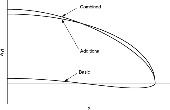
Figure 8.2.1 Illustration of the spanload decomposition for a typical unswept wing, assumed to have a small amount of washout (twist leading-edge down outboard)

Figure 8.2.2 Illustration of the spanload decomposition for a typical aft-swept wing, assumed to have the substantial washout (twist leading-edge down outboard) that is typically required to achieve a favorable total spanload on a swept wing

Figure 8.2.3 Illustration of how a section of an aft-swept wing is “influenced” by more shed vorticity inboard and less shed vorticity outboard compared with an unswept wing

An untwisted aft-swept wing would have a spanload like the additional spanload illustrated in Figure 8.2.2, which is undesirable for several reasons: It produces unnecessarily high induced drag, it leads to excessive bending moments on the structure at high-load conditions, and it produces a tendency for the tips to stall first, which is bad for airplane handling characteristics. To avoid these effects, an aft-swept wing must generally be designed with considerable washout, and thus have a basic spanload with a strong download outboard, to have an advantageous total spanload like that shown in Figure 8.2.2. The favorable spanload that is achieved in this way persists only over a limited range of angle of attack.

8.2.2 Linearized Lifting-Surface Theory

A linearized version of the incompressible inviscid theory is sometimes useful for illustrating trends and providing insight into the behavior of 3D wings, though it suffers a significant loss in physical fidelity. We assume the airfoil sections are thin, and the angle of attack is small, just as we did in 2D (see Section 7.4.1). The flow disturbance produced by the wing is represented by singularities distributed over the chord plane, and the no-through-flow boundary conditions on the wing's upper and lower surfaces are approximated by velocity-slope conditions applied at the chord plane, ignoring the perturbation u, as in 2D. A complication not present in 2D is that the vortex wake must also be modeled. This is done on the assumption that the wake is confined to a sheet that does not distort, and the vortex lines in the sheet stream straight back from where they are shed from the trailing edge, an assumption we'll see again and discuss further in connection with the Trefftz-plane theory of induced drag in Section 8.3.4. A derivation of the integral equations of the theory is given by Ashley and Landahl (1965). We'll not go into the details here; we'll limit our discussion to the general conclusions to be drawn from the theory.

Of course, linearity allows solutions to be constructed by superposition, just as in 2D, and we can look at the effects of various geometry features separately. In 2D we identified separate effects of camber, thickness, and angle of attack. In addition to these three effects of airfoil section shape and orientation, in 3D we have the effects of the wing planform, that is, the distribution of chord along the span, and the sweep, if any. As was the case with regard to spanload decomposition in Section 8.2.1, it should be permissible for the planform to be nonplanar, that is, for the wing to have dihedral and for the dihedral angle to change along the span, which would require the wake sheet to be correspondingly “bent” in rear view. However, references on the theory usually assume that the wing is confined to a single plane, as in Ashley and Landahl (1965).

The three basic sectional effects have different relationships to the effects of planform. Sectional camber and angle of attack both affect lift, and therefore they affect the distribution of vorticity in the wake, which by “induction” affects the velocity perpendicular to the chord plane at other locations on the span. Because of this, sectional camber and angle of attack have effects that are not just local, but spread over the entire planform in a way that depends on the details of the planform. The effects of section thickness are less strongly coupled to the planform. If the wing has a high aspect ratio in addition to being thin, the effects of thickness become effectively local in the limit, depending only on the local streamwise distribution of thickness and the local sweep of the planform, in a manner consistent with the “simple sweep theory” that we'll discuss in Section 8.6.1. In 3D linearized solutions, just as in 2D, airfoil thickness does not affect the distribution of lift.

So in the linear limit, the distribution of lift on a 3D wing depends only on the planform and the distributions of sectional camber and angle of attack. The total lift varies linearly with α, just as it does in 2D, but due to 3D effects the lift curves at different stations along the span can have different slopes and intercepts. The lifting-surface theory predicts both the spanwise and chordwise distributions of load. The downwash is not assumed to be constant in the chordwise direction, so that downwash can affect not just the local effective angle of attack, but also the local effective camber. Still, because of the general linearity that is assumed, the spanload can be decomposed into a basic part at zero lift and a part proportional to angle of attack, as in Section 8.2.1. There we assumed that the aspect ratio is high, and the local downwash affects only the local angle of attack. Here we assume that disturbances are small, and we needn't assume high aspect ratio.

8.2.3 Lifting-Line Theory

The simplest way to predict just the spanload of a 3D wing is the so-called lifting-line theory, in which the chordwise distribution of the load is ignored. The lift is assumed to be concentrated in a single bound vortex, called the lifting line, generally located along the quarter-chord line of the planform, and the vortex-wake sheet is assumed to stream straight back from that, as illustrated in Figure 8.2.4. The bound vortex strength is related to the local lift per unit span using the Kutta-Joukowski theorem, Equation 7.2.1, and as the local lift changes along the span, the change in bound vortex strength is shed into the wake, in keeping with Helmholtz's second theorem (Section 3.3.7). Thus the distribution of vortex strength in the wake sheet is equal to the spanwise rate of change of the bound vorticity. In the early theory developed by Prandtl and his colleagues, the lifting line is assumed to be straight, so that the bound vortex at one part of the span has no influence on the downwash on other parts. The 3D downwash is thus assumed to be only that which is “induced” by the trailing vortex wake, and it is evaluated at the upstream end of the vortex wake, which is by definition on the lifting line itself. Local sections of the wing are assumed to function as 2D airfoils with known sectional (2D) lift curves, with each section operating at an effective angle of attack modified by the local 3D downwash angle.

Figure 8.2.4 Arrangement of the bound vortex at c/4 and the trailing vortex lines in the early development of lifting-line theory. Control points (x) are placed on the bound vortex trailing vortex

The original theory was justified by the informal physical arguments I just outlined. Later, Van Dyke (1964) used the method of matched asymptotic expansions to show that lifting-line theory represents a formally valid approximation in the limit of high aspect ratio and small loading. Early lifting-line theory was used not only to predict spanload, but also induced drag, which we'll consider in Section 8.3.

In the more general case in which the lifting line is not straight, the “contribution” of the lifting line itself to the downwash must be taken into account. The original formulation of lifting-line theory, in which the downwash is evaluated on the lifting line itself, then breaks down because a curved lifting line has infinite self-induced velocity. One way to get around this problem is to introduce a different kind of boundary condition, in which the downwash angle “induced” by the bound and trailing vorticity is evaluated at a downwash line located off of the lifting line and is made to account for both the 3D part of the downwash and the effective sectional angle of attack. This calls for setting the downwash angle equal to the angle of the sectional zero-lift line, and placing the downwash line at the 3/4-chord location, as illustrated in Figure 8.2.5. The 3/4-chord location is chosen because the downwash there, in the 2D case, is equal to the angle of attack of the zero-lift line, provided the 2D lift-curve slope has the linear-theory value of 2π, a result known as Pistolesi's theorem. (The reader can easily verify this using the Kutta-Joukowski theorem, Equation 7.2.1 and the definition of circulation.)

It is clear from Figure 8.2.5 that when the downwash line is located off of the lifting line, the calculation of the downwash “induced” by the trailing vortex lines requires accounting for the additional chordwise segment between the downwash line and the lifting line. In the Weissinger “L” method (Weissinger, 1947), a simplified approximate accounting for the additional segment is used (also see Ashley and Landahl, 1965).

Of course when the lifting line is not straight, the bound vortex influences not just the local 3D downwash angles, but the effective local freestream velocity magnitudes as well. This leads to what is often called a nonlinear lift effect because 3D “induction” now affects the local lift through both the local downwash (and thus the local effective angle of attack and the local Γ) and the local effective U_∞. The local-U_∞ effect can be thought of as either affecting the lift for a given Γ or the Γ required to produce a given lift. This nonlinear effect is generally ignored in lifting-line calculations for several reasons. First, it keeps the equation system linear. Second, it wouldn't be consistent to include this nonlinear effect while assuming the crude lifting-line model for the vortex wake. Finally, the effect has been found to be small for wings of reasonably high aspect ratio (see Eppler, 1997, for example).

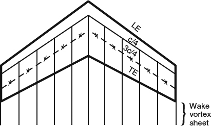
Figure 8.2.5 Arrangement of the bound vortex at c/4, the trailing vortex lines, and the downwash line at 3c/4 in later developments of lifting-line theory. Control points (x) are placed on the downwash line

In numerical implementations of lifting-line theories, the vortex wake is usually discretized as an array of line vortices of finite strength, and the bound vortex is assumed to be straight and to have constant strength between the intersections with the trailing vortices. The boundary condition is enforced at discrete control points between the trailing vortices. In most methods intended for application to nonstraight lifting lines, the control points are placed at the 3/4-chord location as indicated in Figure 8.2.5. Discrete methods have been proposed, however, in which the control point is placed on the lifting line, as in Figure 8.2.4, even though the lifting line is not globally straight (Phillips and Snyder, 2000, for example). The problem that this incurs is hidden from view because the discrete straight lifting-line segments artificially mask the problem of infinite velocity that we discussed above. But the problem is still there in the limit as the segment length goes to zero. Thus locating the control points away from the bound vortex is still the only way to have a general formulation that doesn't behave badly as the discretization is refined.

Even when a downwash line separate from the lifting line is used, lifting-line theory in effect assumes that the downwash due to finite span doesn't vary much in the chordwise direction, over the whole chord of the section at any given station along the span. This is not a bad assumption for high-aspect-ratio wings with reasonably straight quarter-chord lines, and in such cases, the theory can provide fairly accurate results. However, for swept wings, which generally have a pronounced kink in the quarter-chord line at the center station, the assumption is poor for the inboard part of the wing, and Thwaites (1958) goes so far as to state that lifting-line theory is “completely unjustified” for swept wings. Still, it is often used for swept wings anyway, and semi-empirical adjustments to improve its accuracy in the neighborhood of the kink in the lifting line have been proposed, as in Barnes (1997).

8.2.4 3D Lift in Ground Effect

In Section 7.4.9, we saw that as an airfoil in 2D flow gets closer to a ground plane, the lift is first reduced and then increased. For a 3D wing, a ground plane has a 3D effect on lift, which often overwhelms the 2D effects. A ground plane in 3D also affects the induced drag, as we'll see in Section 8.3.9.

When a wing flies close to the ground, the no-through-flow condition at the ground forces the flowfield around the wing to change in a way that generally increases the lift at a given angle of attack or reduces the angle of attack required for a given lift. One way to look at this is that the ground has the effect of inhibiting vertical velocity throughout the field and therefore reduces the 3D downwash in which the wing is flying.

A second way to look at it that also provides a basis for simplified quantitative calculations is to invoke the idea of images. A simple way to ensure that the no-through-flow condition at the ground is satisfied is to place an image of the vortex system below the ground, as shown in Figure 8.2.6. Then part of the downwash “induced” by the real vortex system can be seen to be canceled by the upwash “induced” by the image system. A single horseshoe vortex and its image could be used for this purpose, but the physical fidelity would be poor. A model with a more realistic distribution of the shed vorticity, but ignoring rollup, like that used in lifting-line theory (Section 8.2.3) or an inviscid panel method (Chapter 10), would provide somewhat better fidelity, and the effect on lift could still be readily calculated. The change (increase) in lift at a fixed angle of attack for a planar wing with a rectangular planform of aspect ratio 10 and no twist is shown in Figure 8.2.7, as calculated by a panel method with a nondistorting wake sheet. In this example, the 2D lift decrease is more than offset by the 3D lift increase due to the reduction in downwash. We can look at finite span as having two effects that work in the same direction. First, finite span introduces 3D downwash, which is reduced by the presence of the ground. Second, finite span also attenuates the 2D effects of the ground because an image bound vortex of finite span has less “influence” than one of infinite span.

Figure 8.2.6 Bound and trailing vortex system of a wing flying in ground effect, and its image under the ground plane

Figure 8.2.7 The increase in lift of a wing in ground effect. Results of a lifting-line calculation for a rectangular planform AR = 10, no twist. C_l = 0.81 out of ground effect

Comparing Figure 8.2.7 for a 3D wing with Figure 7.4.35 for a 2D airfoil, it appears that for wings of ordinary aspect ratio the effect of the ground on lift is dominated by finite-span effects. Note that 2D lift in Figure 7.4.35 is decreased until h/c goes below 0.3, which corresponds to h/b = 0.03 in Figure 8.2.7. Above this value, the 3D effect in Figure 8.2.7 clearly dominates. Presumably at some point below h/c = 0.3, the 2D effect would begin to contribute more to the lift increase than does the 3D effect, but this range is seldom of practical interest. For a wing with significant dihedral, or sweep combined with angle of attack, such low values of h/c would not be reachable over much of the span, even without a landing gear.

Depending on the geometry of the wing, ground effect can change the shape of the spanload, and if the wing is swept, it can cause substantial changes in the pitching moment. A swept-wing airplane with an aft tail can experience complicated changes in its lift curve and pitching moments as functions of height when in close proximity to the ground plane.

8.2.5 Maximum Lift, as Limited by 3D Effects

In Sections 7.4.3 and 7.4.4, we looked at how the maximum lift of 2D airfoils, both single-element and multiple-element, is limited by boundary-layer separation. It turns out that sectional maximum lift, as limited by boundary-layer separation, is also generally the limiting factor for 3D wings. However, in the late 1950s, there was considerable interest in flap systems that used active jet blowing to control separation (“blowing BLC”) and, when the blowing was very strong, to directly enhance the circulation around the airfoil (the “jet flap”). In such cases, the 3D downwash field can become the factor that limits the maximum lift of a 3D wing.

As we saw in Section 8.1, the downwash associated with finite span has the effect of tilting the lift vector back. The horizontal component is felt as induced drag, and the vertical component is reduced to something less than the magnitude of the force. Furthermore, the magnitude of the force for a given circulation (bound vortex strength) is reduced because the vortex wake is generally tilted downward, so that the velocity “induced” by it has a forward component that subtracts from the effective freestream velocity. Thus when we try to increase the circulation on a 3D wing, by whatever means, the tilting back of the force vector and the reduction of the effective freestream velocity both increase, and presumably at some point the vertical component (the lift) should stop increasing, thus defining a maximum achievable lift limited by 3D downwash.

Davenport (1960) looked at three highly idealized models for this effect that had been proposed by others and found that their predictions varied widely depending on their assumptions about the wake. By their nature, such theories predict maximum lift proportional to span, independent of wing area. Thus when normalized by wing area, they all predicted C_Lmax proportional to aspect ratio. However, the constants of proportionality ranged from about 0.8 to 2.0. Davenport proposed a model of his own that gave a result at the high end of this range, but also concluded that the effect depends strongly on the details of the flow, especially as reflected in the tilt of the wake near the airfoil. In any case, the range of C_Lmax predicted by these models is so high as not to be achievable without some form of active flow control.

8.3 Induced Drag

In Section 8.1.1, we looked at the flowfield around a lifting wing of finite span, and we saw how the lift vector is tilted back, making a contribution to drag that we call induced drag. In this section, we delve into the related quantitative theory, which we should note at the outset requires some degree of idealization. Recall that in Section 6.1.3 we discussed how it is essentially impossible to decompose the total drag force on a body rigorously into separate contributions based on the different flow mechanisms responsible. In the theories of induced drag in this section, we'll sidestep that issue by assuming that the flow is inviscid and that there are no total-pressure losses through shocks, so that the induced drag is the only drag “component” present. So we must keep in mind that quantifying induced drag as a separate “component” of the drag force is an idealization.

But assuming inviscid flow in the theory doesn't cost us as much in terms of accuracy as one might think initially. We can use induced-drag theory without necessarily assuming that the entire flowfield must be consistent with inviscid flow. For example, in theories in which the lift distribution on the wing is an input, we can use a lift distribution consistent with the real flow, including viscous and transonic effects. Because we reintroduce realism in this way, the conclusions we draw from induced-drag theory can be reasonably accurate in most of the more general situations we'll encounter in practice. Just keep in mind that the theory of induced drag generally ignores some physical complications and incurs at least some small error as a result.

8.3.1 Basic Scaling of Induced Drag

By appealing to the idealized lifting-line model for the flow around a simple wing illustrated in Figure 8.2.4, we can deduce how induced drag should scale with the lift, the flow conditions, and the dimensions of the wing. If Γ is the centerline circulation, the total lift will go as ρU_∞Γb. As we argued in Section 8.1.1, the wing is flying in a downwash field of its own making, as illustrated in Figure 8.1.2. We'll therefore assume that the induced drag is given by the lift tilted back through an average downwash angle ε, or D_i ∼ Lε. For the simple straight lifting line in Figure 8.2.4, the lifting line “induces” no downwash on itself, and we need only consider that “induced” by the trailing vortex wake, for which the downwash velocity goes as Γ/b, and ε goes as Γ/U_∞b. Combining these so as to eliminate Γ, we get

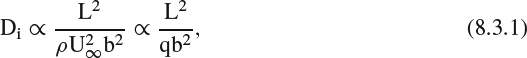
which illustrates some important trends. Induced drag increases rapidly with increasing lift and decreases rapidly with increasing span. Flying at high altitude (small ρ) or low speed increases the induced drag. Induced drag is the one major part of the drag of an airplane that decreases with increasing speed, in contrast with the viscous drag that we considered in Chapter 6, which tends to increase roughly as . Given these two opposing trends, the drag tends to be dominated by induced drag at low speeds and by viscous drag at high speeds, with a drag minimum in between, as illustrated in Figure 8.3.1. In this illustration, the ideal and dependences were assumed, so that the minimum total drag occurs where each component contributes half the total. For real wings, the nonideal behavior of the profile drag tends to drive the minimum drag to a higher speed (lower C_L), as we discussed in Section 7.4.2. Nonideal behavior of the induced drag can shift the minimum in either direction.

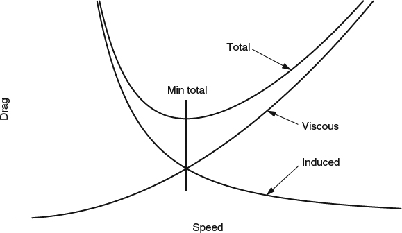
Figure 8.3.1 Schematic drag-versus-speed curve for an airplane, illustrating the induced and viscous contributions

Note that as a result of our lifting-line assumptions the induced drag depends on the span of the wing and not the area. This also holds in the Trefftz-plane theory, which we'll discuss in Section 8.3.4 and which provides sufficient accuracy for nearly all practical predictions of induced drag. So for practical purposes, induced drag does not depend at all on wing area. This sets induced drag apart from the lift, viscous drag, and pitching moment, which tend to be proportional to area, and introduces a practical problem that has been a source of some confusion. Most of our dealings with these forces are in terms of the dimensionless coefficients C_L, C_D, and C_M. Because all of the raw dimensional forces other than the induced drag are roughly proportional to qS, nondimensionalizing by qS is the only choice that makes sense. But then to be consistent, we must nondimensionalize induced drag the same way, getting

So unfortunately, nondimensionalizing induced drag by wing area makes it look (misleadingly) as if the induced drag depends on wing area, or aspect ratio. The appearance of aspect ratio in such formulas is a red herring, an artifact of a nondimensionalization that is more appropriate for other quantities.

8.3.2 Induced Drag from a Farfield Momentum Balance

We can derive a very general formula for the induced drag based only on the farfield flow, with only minimal assumptions about how the flow behaves:

1. The flow is steady and inviscid, and density variations in the farfield can be ignored, so that we can use the steady, incompressible form of Bernoulli's equation.
2. Velocity disturbances in the farfield tend to zero except in the neighborhood of a vortex wake that is convected indefinitely downstream but does not spread out without bound in the other directions. This is consistent with the general character of the vortex wake that we saw in Section 8.1.2.
3. The wake flowfield is established during the wake rollup process, which is effectively completed within the relative nearfield of the airplane, so that the wake becomes unchanging from there downstream, except for a downward drift.

We orient the x-axis in the flight direction and tie our reference frame to the airplane in steady flight, so that the freestream velocity is U, and the velocity everywhere else is (U, V, W) = (U + u, v, w). We expect the wake far downstream to carry a significant u disturbance, including a nonzero integrated u, and thus a net flight-direction mass flux (remember the axial jets in the rolled-up vortex wake in Figure 8.1.9). This flight-direction mass flux will enter into the momentum balance in any control volume with a far-downstream boundary, and it must come from somewhere. A wake with a jet, as in Figure 8.1.9, requires flow to converge toward the region where the wake is forming, while a wake with a velocity deficit (negative u) would require flow to diverge. From far enough away, this will look like a single sink or source located in the neighborhood of the airplane, because we have assumed that wake development is completed not far from the airplane. In our derivation of the simplified formula for viscous drag (Equation 6.1.3) we also had to account for a balancing mass flux, in that case a source.

In the momentum balance for a general control volume surrounding the airplane, the pressure and momentum-flux disturbances in the neighborhood of where the wake leaves the downstream boundary are obviously significant. The significance of disturbances elsewhere is not quite as obvious. The velocity and pressure disturbances associated with the source or sink are spread diffusely in all directions and die off with increasing distance, but it turns out that they don't die off fast enough that their integrated effects can be neglected, no matter how far away we put the boundaries. Having to deal with the source or sink terms complicates the analysis a bit, and the source or sink ends up dividing up its contributions through the pressure and the momentum flux differently depending on the shape of the control volume. The total contribution of the source or sink to the inferred drag must of course be the same regardless of how the control volume is shaped. We can get the right answer for the total contribution of the source or sink and simplify the algebra considerably, if we assume a particular kind of shape for the control volume.

We give the control volume a general cylindrical shape as in Figure 8.3.2, with an upstream boundary, a downstream boundary, and lateral/top/bottom boundaries that simply need to form a general cylinder (not necessarily circular) parallel to the x-axis.

The cross-section shape in the y-z plane can be anything, as long as the cross section is large enough that the downstream boundary captures all of the significant pressure and velocity disturbance associated with the vortex wake. Now we take the upstream and downstream boundaries to large distances compared to the other dimensions of the control volume, but not so large that downward drift of the vortex wake carries it out through the cylindrical boundary instead of the downstream boundary. To proportion the control volume in this way requires a small inclination angle for the vortex wake. This requires that the spanloading on the wing producing the wake not be too large, which is more restrictive than our original assumptions (1–3). This does not mean we are assuming that u, v, and w are small in the vortex wake. The assumptions regarding the shape of the control volume lead to the following simplifications:

Figure 8.3.2 Cylindrical control volume for deriving Equation 8.3.5 for the induced drag from a far-field momentum balance

1. The cylindrical part of the boundary makes no contribution to the momentum balance through the pressure, because its normal is everywhere perpendicular to the x-axis.
2. At the upstream and downstream boundaries we can neglect the pressure and velocity disturbances due to the source or sink.
3. The strength of the source or sink can be calculated from the integrated u deficit or excess at the downstream boundary, designated T, due solely to the vortex wake:

The total effect of the source or sink on the momentum balance is due to the momentum flux through the cylindrical boundary and is given by .

With these simplifications, the momentum balance becomes

After we use the steady, incompressible Bernoulli equation to express the pressure in the wake terms of U, u, v, and w, and simplify, we obtain

The negative sign of the u² term is a little disturbing at first glance, because it means that the integrand is not positive-definite and raises the concern that the drag might not be always be positive. A rigorous argument by Spalart (2008) indicates that this is not a problem. An informal argument that reaches essentially the same conclusion goes as follows:

In the next two theoretical models that we'll consider, we'll ignore the downward drift of the wake and the associated general downward tilt of the vortex lines. We'll also ignore any other deviation of the vortex lines from the freestream direction, as, for example, in the helical alignment of the vortex lines in the cores shown in Figure 8.1.5. The farfield wake then has no u disturbance associated with it, and the u² term in Equation 8.3.5 is zero. We can then interpret the induced drag as being accounted for by the kinetic energy left behind in successive slices of the flow in the wake.

8.3.3 Induced Drag in Terms of Kinetic Energy and an Idealized Rolled-Up Vortex Wake

Here we make the same basic assumptions as we did leading to Equation 8.3.5, and we calculate the velocities in Equation 8.3.5 using the Biot-Savart law, based on simple assumptions regarding the distribution of vorticity in the wake. We ignore the tilt of the wake and the circumferential component of the vorticity in the vortex cores. The simplest model for a rolled-up vortex wake is a pair of line vortices, but the kinetic energy integral in the neighborhood of a line vortex is infinite, which rules this model out for evaluating induced drag in terms of kinetic energy. For the kinetic energy to be finite, the vorticity must have finite strength and must therefore be spread out over a finite area. The simplest vortex model that does this is the so-called Rankine vortex we described in Section 3.3.8 and Figure 3.3.8f, in which the vorticity is assumed constant inside of a circular core of radius r_c, outside of which the flow is assumed irrotational. So a simple model for the rolled-up wake behind a lifting wing consists of two Rankine vortices of strength Γ_o and radius r_c with their centers separated by a spanwise distance b_o, as shown in Figure 8.3.3. Now three parameters, Γ_o, b_o, and r_c, are sufficient to determine the drag. If Γ_o, b_o, and the drag are known, r_c can be adjusted to match the drag. This idea of adjusting the core radius to match the drag began with Prandtl (see Spalart, 2008).

One problem with a wake model based on Rankine vortices is that the combined flowfield associated with two such vortices is not consistent with maintaining the circular boundaries of the cores over time. (The flow outside the Rankine cores should be the same as the flow around two point vortices, and this flow does not have circular streamlines of radius r_c centered on the vortices.) This has not discouraged use of the model, however, and the problem has been sidestepped in at least two different ways, neither of which is entirely satisfactory.

Spreiter and Sacks (1951) sought to work around the problem by taking advantage of the fact that the streamlines of the flow around two point vortices are actually circular, just not all centered on the vortices. They noted that only the streamline circles of zero radius are centered on the vortices and that as we look at larger radii, the streamline circles have centers shifted increasingly outboard. They therefore placed the Rankine cores so that their boundaries matched the streamline circles of radius r_c, so as to align the core boundaries with streamlines of the irrotational flow surrounding the cores. The trouble with this is that when the cores are positioned in this way, their centers don't coincide with the locations of the original point vortices, so that the flow they “induce” isn't consistent with the assumed flow outside the cores.

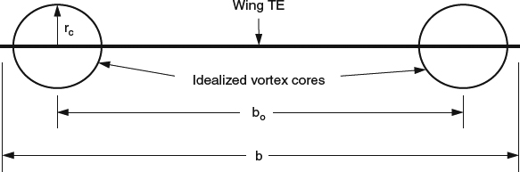
Figure 8.3.3 Idealized model for the rolled-up vortex wake used in the theories of Spreiter and Sacks (1951) and Milne-Thomson (1966) (drawn to scale for r_c/b = 0.0855, r_c/b_o = 0.1089)

Milne-Thomson (1966) also assumed the flow outside the cores is consistent with two point vortices but did not shift the centers of the Rankine cores outboard from the locations of the point vortices, arguing that this was valid as long as the core radius is small compared to the separation. However, the core radius he finally deduces turns out not to be that small. So this is also an inconsistency, just a different one from that of Spreiter and Sacks.

In spite of the inconsistencies of both of these models, the calculations for the kinetic energy can be carried out. For the Milne-Thomson version, the result is

where Γ_o is the circulation of the cores. To see what this implies about the size of the cores behind a typical wing, assume an elliptic load distribution on a wing of span b, for which the classical theory of Section 8.3.4 gives

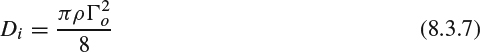
and

Then the core radius is given by

The model is thus kinematically inconsistent. But the more serious problem with Rankine vortex cores is that they don't model the flow in the rolled-up wake behind a wing well at all, as we saw in Figure 8.1.8.

8.3.4 Induced Drag from the Loading on the Wing Itself: Trefftz-Plane Theory

Here we seek to infer induced drag from the loading on the wing itself, without laboriously computing the entire flowfield. This requires making simplifying assumptions not just about the farfield wake, but regarding the development of the wake all the way from where it leaves the wing trailing edge. Trefftz-plane theory does this by ignoring the rollup of the trailing vortex sheet and assuming instead that the vortex lines stream straight back in the freestream direction from where they are shed at the trailing edge, as illustrated in Figure 8.3.4. This theoretical framework was established in the early 1900s (Prandtl and Tietjens, 1934) and is still in use today. The formal justification is that neglecting the deformation of the wake should be valid in the limit of small loading or high aspect ratio. The practical justification is that the resulting theory gives reasonably accurate results for practical loadings and aspect ratios.

A real vortex wake, outside of the rolled-up portion at the outboard edge, is a finite-thickness shear layer that aligns itself with the flow on both sides, has no flow through it, and supports very little pressure difference across it. At the next level of idealization, this shear layer would be modeled as a thin vortex sheet that is also a stream surface of the flow, having, by definition, no flow passing through it and no force on it. No force means there can be no pressure jump across the sheet. In a shock-free inviscid flow, no pressure jump means there can be no jump in velocity magnitude across the sheet, only a jump in velocity direction. No jump in velocity magnitude in turn requires that the vortex lines in the sheet be aligned parallel to the average of the velocities on the two sides of the sheet (If the vortex lines were not aligned in this way, there would have to be a jump in velocity magnitude, as we noted in Section 3.3.8, and thus also a jump in the pressure, violating our no-force condition). So a vortex wake modeled as a force-free vortex sheet must satisfy requirements on both the shape of the sheet and on the alignment of the vortex lines in the sheet.

Unlike this ideal force-free vortex sheet, the assumed wake sheet in Trefftz-plane theory, made up of vortex lines aligned with the free-stream direction, will generally have a nonzero component of velocity perpendicular to the vortex lines, both from flow passing through the sheet and from vortex lines not being appropriately aligned within the sheet. Whenever there is a velocity component perpendicular to vortex lines, and the vortex lines are not being convected with the flow, the Kutta-Joukowski theorem requires that there be a “lift” force perpendicular to both the velocity and vorticity vectors. Thus the nonzero component of velocity perpendicular to the vortex lines results in local forces exerted on the wake that are small for a typical high-aspect-ratio wing, but nonzero. Because these forces must be perpendicular to the vortex lines, they make no contribution in the drag direction. So the wake in Trefftz-plane theory is not force free, but it is drag free.

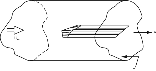
Figure 8.3.4 Assumed wake model in the Trefftz-plane theory of induced drag, with the vortex lines running straight back in the freestream direction

Kroo (2001) argues that because the wake assumed in Trefftz-plane theory is drag free, Trefftz-plane theory incurs no error in the drag calculation, and that it should therefore give the same result for the induced drag as a calculation that takes into account realistic distortions of the wake. I would argue that a drag-free wake does not guarantee this level of correctness, but only consistency in the sense that the total drag in the field does not contain a contribution from drag on the wake. Consistency in this sense then means that the farfield drag determination would agree with the drag determined by surface-pressure integration, if the flow is inviscid and shock-free, but it does not preclude an error in the drag, due to the incorrect positioning of the wake. The error due to the simplified wake model will generally be nonzero, though in most practical cases it is likely to be small. This is an issue we'll take up again in Section 10.4.3 when we discuss 3D CFD codes based on potential-flow theory, in which the wakes of lifting surfaces are often modeled in a way that is equivalent to the assumptions of Trefftz-plane theory.

Trefftz-plane theory is applicable to a lifting system that can be made up of one or more lifting surfaces, each of which can be either planar or nonplanar. The theory takes the spanwise distribution of lift to be known and determines the induced drag either locally in terms of the backward tilt of the lift vector distributed along each lifting surface, or globally in terms of the total kinetic energy in a cross-flow plane (the Trefftz plane) far downstream. The local determination defines both the spanwise distribution of induced drag along the surfaces and the total, while the global determination defines only the total. The total induced drag determined either way is the same.

The flowfield velocities that are used in calculating the drag do not come from solving the equations of motion in the flowfield, but are inferred from the idealized model of the vortex wake, through the Biot-Savart law. The theory thus depends on inferring velocity from vorticity, which is justified mathematically, but obscures the physical cause-and-effect relationships. As a result, the physical understanding provided by the theory is not all that we might hope for. While the theory makes very clear the relationship between the down-wash distribution and the distribution of drag, it does not provide much intuitive physical understanding as to why a particular lift distribution produces a particular downwash distribution. Although the physical understanding it provides is minimal, Trefftz-plane theory is very valuable for its quantitative predictions, and we depend heavily on it, for nearly all predictions of induced drag. Historically, its predictions have been found to agree reasonably well with drag measurements both in the wind tunnel and in flight.

Note that in our simplified model of the wake in Figure 8.3.4, the wake sheet forms a general cylinder (“general” in the sense of not necessarily circular) defined by the trailing edge and having generators in the direction of the freestream. The distributions of vortex strength in the wake sheet and the bound vorticity on the wing are defined consistently with the Kutta-Joukowski theorem (Equation 7.2.1), and Helmholtz's second theorem (Section 3.3.7), in the manner we described in connection with the lifting-line theory in Section 8.2.3. Given the spanwise distribution of lift and the geometry of the trailing edge, the distribution of vorticity in the wake is defined, and the downwash at each station along the span of the wing itself can be calculated using Biot-Savart. This determines the local backward tilt of the lift vector and the local induced drag. In the literature, this local determination of the drag seems to be discussed only in the context of straight, unswept wings, for which the contribution to the downwash from the bound vorticity on other parts of the span can be ignored. For example, Milne-Thomson (1966), in his Section 11.22, evaluates the down-wash at the trailing edge, which is assumed to be straight, using only the contribution of the trailing vorticity. To extend this treatment to swept wings or wings that are otherwise not straight would entail the same inaccuracies we discussed in connection with lifting-line theory in Section 8.2.3. Because of these inaccuracies, local determinations of induced drag are not usually pursued for wings that are not straight, and for most purposes, it is only the total induced drag that matters anyway.

The total induced drag can also be determined from the flowfield far downstream using Biot-Savart and Equation 8.3.5. One way of expressing the result is through the following integral expression:

where the integration is over the line or curve where the undeformed trailing vortex sheet intersects the Trefftz plane, and v_n is the velocity “induced” by the wake perpendicular to the line or curve. The factor of 1/2 is required when v_n is evaluated far downstream, where the wake vortices appear infinite, instead of at the wing itself, where the wake vortices appear only semi-infinite. Only the trailing vortex wakes enter into this integration for the total induced drag, and given our idealized model for the wakes, the distribution of vortex strength depends only on the spanwise distribution of lift and on the shapes of the lifting surfaces as seen in rear view, the so-called “Trefftz-plane view.” Thus for a given spanwise distribution of lift, the total induced drag is independent of the fore-and-aft arrangement, including the sweep, of the parts of the lifting system. This result was originally derived with reference to a biplane and is referred to as Munk's stagger theorem (see Kroo, 2001). Fore and aft disposition affects both the spanwise distribution of induced drag on individual lifting surfaces and the distribution of drag among multiple lifting surfaces, but not the total, provided the spanwise distribution of lift is held constant. Note that this doesn't generally apply when lifting surfaces of fixed shape are moved fore and aft relative to each other because in that case the lift distributions generally change. To keep the lift distributions constant as surfaces are moved fore and aft, as required by the stagger theorem, generally requires changes in twist and/or camber.

Numerical methods for calculating the rollup of the wake sheet in potential flow that in principle predict induced drag with higher fidelity than Trefftz-plane theory are available, but they are not that widely used when the objective is to study induced drag. CFD methods based on Euler or Navier-Stokes equations predict the entire flowfield in detail, including the rollup of the vortex wake. However, flow solutions provided by these methods present us with the same problem we encountered with the real flow; that is, how do we define what part of the total drag is induced drag? It is telling that when users of high-fidelity CFD codes want a separate number for the induced drag predicted by their solutions, they usually plug their calculated lift distributions into Trefftz-plane theory.

8.3.5 Ideal (Minimum) Induced-Drag Theory

What is the minimum induced drag that a wing can have? This question makes sense only if we constrain the total lift to a nonzero value, because if the load is zero everywhere, the induced drag is zero. So for a given configuration of lifting surfaces as viewed in the Trefftz plane, Equation 8.3.10 defines an optimization problem that can be solved for the minimum induced drag, and for the spanload that goes with it, provided we constrain the total lift. When total lift is the only constraint, and minimum induced drag is the only objective, the results of this optimization are called the ideal induced drag and the ideal spanload. There are various ways this optimization problem can be solved, sometimes analytically, but usually numerically. We'll forego the details here and discuss only the general results and conclusions of the theory.

One general conclusion has to do with the normalwash in the Trefftz plane. If the spanload is ideal, the component of the wake-induced velocity in the direction perpendicular to the wake cut in the Trefftz plane is related to the local dihedral angle θ of the cut:

This relation was derived by Munk (1921) and is often referred to as Munk's minimum-induced-drag criterion. A normalwash distribution obeying this rule is illustrated in Figure 8.3.5.

For a planar wing, θ is zero, the normalwash is constant and is the same as the down-wash, which, according to the theory, requires an elliptic lift distribution, as illustrated in Figure 8.3.6.

In this case, we have the classic result for the induced drag:

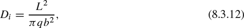
or in dimensionless terms:

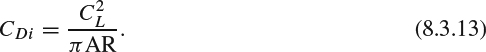
This, of course, reflects the same scaling we deduced in Equations 8.3.1 and 8.3.2 and fills in the constant of proportionality for one particular case. The dimensionless form, Equation 8.3.13, is the better known of the two, which is unfortunate. It gives the misleading impression that aspect ratio plays an important role in induced drag. As we saw earlier, the aspect ratio in Equation 8.3.13 is really a red herring, an artifact of the nondimensionalization. It is clear from Equations 8.3.1 and 8.3.12 that the induced drag force depends on span, not on aspect ratio.

Figure 8.3.5 Illustration of the normalwash rule, Equation 8.3.11, associated with an ideal spanload. The vectors drawn here show only the normal component of the velocity

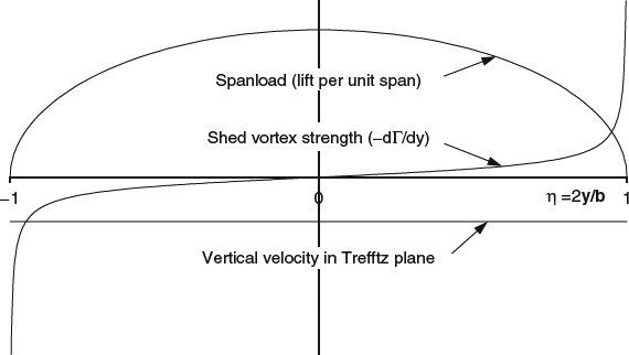
Figure 8.3.6 Elliptical spanload and constant downwash of an ideally loaded planar wing

So the well-known elliptic spanload is “ideal” for a planar (flat) wing. For nonplanar configurations, the ideal spanload is not generally elliptic, but it is easily calculated for a given geometry. With a vertical winglet added, for example, the ideal spanload shows less lift inboard and more lift outboard, relative to elliptic, with a certain optimum distribution on the winglet itself, as shown in Figure 8.3.7. Note that “lift” in this context refers to the aerodynamic force perpendicular to the wing locally, which in the case of the vertical winglet is a horizontal force inward. Also note that according to Equation 8.3.11 the normalwash produced in the Trefftz plane by a vertical winglet is zero. If the wing and winglet are unswept, the normalwash at the surfaces themselves is half what it is in the Trefftz plane, because the wing and winglet “see” only a semi-infinite wake sheet, whereas the Trefftz plane “sees” a wake sheet that is effectively infinite both fore and aft. This means that the winglet itself experiences no sidewash, or that the load on the winglet cancels the sidewash that would be there in the absence of the winglet. This is a point we'll consider further in Section 8.4.2 in connection with the common misunderstanding that wingtip devices like winglets generally produce induced thrust.

Figure 8.3.7 Ideal spanload for a wing and vertical winglets, compared with the elliptic ideal loading of a planar wing

Relative to the “ideal” spanloads we've discussed here, the spanloads used on real wings are usually modified somewhat to reduce bending loads at highly loaded structural critical conditions and allow a lighter wing structure, at the expense of a slight increase in drag in cruise. The presence of a fuselage and wing-mounted engines also tends to alter the spanloads on real wings, an effect for which we'll discuss one idealized model next.

The fact that downwash is constant for an elliptically loaded planar wing, both at the wing itself if it is unswept, and in the Trefftz plane, might lead us to expect that the vortex wake would remain undistorted, as Trefftz-plane theory assumes. This expectation is unrealistic for more than one reason. Remember from our discussion of the vortex wake in Section 8.1 that Spalart (1998) showed that it is not possible for the wake to remain undistorted at the outer edge. And the “induction” by the trailing vortex sheet is not the only contribution to the downwash. The bound vorticity “induces” a nonuniform downwash that distorts the wake in the nearfield of the wing. So uniform downwash in the Trefftz plane doesn't mean that the wake remains undistorted. And there is another important way in which the undistorted wake assumed in the Trefftz-plane theory is unrealistic. The farfield descent rate of an undistorted wake sheet of an elliptically loaded wing, implied by its own self-induced velocity, is much higher (a factor of π²/2 ≈ 4.9) than the descent rate of the real rolled-up wake.

8.3.6 Span-Efficiency Factors

Equations 8.3.12 and 8.3.13 apply to an ideal elliptically loaded planar wing. If the wing is nonplanar or the spanload is nonideal, the induced drag will differ from the planar ideal. It is often convenient to relate the actual drag to the planar ideal through the induced-drag span-efficiency factor, e, defined by

For a planar wing, the actual induced drag is always greater than or equal to the ideal, so that e is always less than or equal to one. For a nonplanar wing, the induced drag can be less than the planar ideal, so that e can be greater than one.

Another “efficiency factor,” called the Oswald efficiency factor, e_o, takes into account the variation with C_L of the total drag, including the viscous profile drag. It is defined in practice by fitting the total drag polar with the following expression:

Recall from Section 7.4.2 that the sectional profile drag polar of a 2D airfoil typically has a roughly parabolic variation in the low-to-moderate range of C_L. The integrated profile drag of a 3D wing tends to behave similarly, so that the inclusion of the profile drag makes the coefficient of the term in Equation 8.3.15 larger than it would be for induced drag alone. Thus for wings with ordinary airfoil sections, e_o is usually smaller than e.

An important point to note about the two efficiency factors is that e_o is defined such that it can in general be determined by a curve-fit of a known total-drag polar, though the value generally depends on what part of the polar is fitted, while e cannot generally be determined just from the total drag. Sometimes this point is overlooked, and e_o is confused with e. An example of this is seen in the claims of low induced drag that were made for the Winggrid wingtip device (La Roach and La Roach, 2004), which consists of a cascade of constant-chord airfoils appended to the tip of a conventional wing. The cascade almost certainly has high profile drag at low C_l s, and as a result, a range of C_l over which the profile drag decreases with increasing C_l. This would make that portion of the total polar shallower than it would be with induced drag alone, rather than steeper, as would usually be the case with an ordinary single-element airfoil. The author apparently fitted this portion of the polar and obtained a high value of e_o, from which he inferred a low value of induced drag that is probably not realistic.

8.3.7 The Induced-Drag Polar

If we assume that e is constant, independent of C_L, Equation 8.3.14 implies that the induced-drag polar is a simple parabola, with zero induced drag at zero lift. But for this to be true the wing would have to maintain the same spanload shape as C_L varies, which a real wing doesn't generally do. The spanload of a real wing can have a complicated variation with angle of attack, due to transonic and viscous effects, and the induced-drag polar will be correspondingly complicated. But even in the absence of nonlinear effects, the spanload of a twisted wing changes shape with angle of attack, and it is instructive to look at the trends predicted by simplified theories. Combining Trefftz-plane theory for the total induced drag with the decomposition of the spanload into basic and additional parts (Section 8.2.1) leads to a prediction of the induced-drag polar (Rubbert, 1984). In terms of the bound circulation, the spanload decomposition can be expressed as

where Γ_o and α_o are the circulation distribution and angle of attack of the wing when the total lift is zero. Substituting this into the total-induced-drag integral, Equation 8.3.10, and doing some rearranging yields the result that the induced-drag polar is parabolic:

for a general twisted wing, where C_Dio and A₁ are zero if Γ_o is zero everywhere. Thus for an untwisted wing, we would have only

Equation 8.3.17 can be rearranged in terms of C_L(C_Dimin) and C_Dimin, the lift and drag coefficients at the minimum of the polar:

where e_NT is the span-efficiency factor of the corresponding untwisted wing.

Figure 8.3.8a illustrates the parabolic induced-drag polar of a swept, twisted wing. Note that in this polar, the C_Dio term is significant, but the A₁ term is relatively small, which seems to be typical of most real wings. The spanload-efficiency factor e in Figure 8.3.8b varies dramatically with C_L, showing what a serious mistake it is to assume e is constant, even though e_NT is constant. And this is another example in which confusing e_o with e and determining e by a curve-fit to the term in the total drag would be a mistake in that it would miss the C_Dio part of the induced drag.

8.3.8 The Sin-Series Spanloads

There is a simple trigonometric series for representing the spanload of a planar wing that has some very useful properties (see Durand, 1967b). The lift per unit span is represented in terms of a series with coefficients A_i:

or in dimensionless form:

where ψ is the transformed spanwise coordinate:

Figure 8.3.8 Induced-drag behavior of a swept, twisted wing according to Equation 8.3.17. (a) The induced-drag polar. (b) The corresponding span-efficiency factor e

The integrated lift involves only the first term of the series:

or in dimensionless form:

Only the odd-numbered terms are usually used, as they are the ones that are symmetrical about the center plane. The first three odd-numbered terms are plotted in Figure 8.3.9. The first term represents an elliptic loading, while all the higher terms carry no net lift, which is why they don't appear in Equation 8.3.24.

When the spanload expression 8.3.20 is introduced into Equation 8.3.10 for the induced drag, the result is

or in dimensionless form:

so that the span efficiency factor is given by

The wing-root bending moment M_BR due to the lift distribution also has a simple expression:

The first two odd-numbered terms of the series provide a convenient way to generate span-load shapes that are compromised from elliptical to reduce bending moments and thus reduce wing structural weight. Using just the first two terms gives the least increase in induced drag for a given reduction in root moment. A family of such spanloads is illustrated in Figure 8.3.10, and the e-versus-bending moment curve is plotted in Figure 8.3.11. Note that induced drag increases (e decreases) whether root bending moment decreases or increases, consistent with fact that the baseline spanload is the elliptic optimum. Note also that e decreases only quadratically with the deviation from the optimum, something we'll see again in connection with the effect of a tail or canard on induced drag in Section 8.3.11. The first two odd-numbered terms also provide a convenient way of sketching spanloads of different shapes for illustration purposes, which was used in generating the sketches in Figures 8.2.1 and 8.2.2.

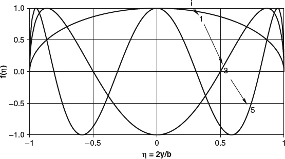
Figure 8.3.9 The first three odd-numbered terms in the sin-series expansion for representing spanloads

Figure 8.3.10 A family of spanloads compromised from elliptic to reduce wing-root bending moment using the first two odd-numbered terms in the sin-series expansion

Figure 8.3.11 The variation of e with M_BR for spanloads using the first two odd-numbered terms in the sin-series expansion

8.3.9 The Reduction of Induced Drag in Ground Effect

When a wing flies close to the ground the no-through-flow condition at the ground forces the flow field around the wing to change in a way that reduces the downwash in which the wing is flying. This has the general effect of increasing the lift at a given angle of attack, as we saw in Section 8.2.4, and reducing the induced drag for a given lift.

For calculating this reduction in induced drag, it is helpful to invoke the idea of images, just as it was for calculating the increase in lift in 3D ground effect in Section 8.2.4. A typical result of a panel-method calculation is shown in Figure 8.3.12. Note that both C_Di and the change ΔC_Di due to ground effect are of order , so that the drag reduction expressed as a ratio C_Di/C_Di∞ doesn't depend on C_L.

It's clear from Figure 8.3.12 that the ground produces substantial percentage reductions in induced drag when h/b < 1. This can be important in many types of flight on minimal power, as, for example, in human-powered flight and the long-distance flight of some birds over water. The idea of specifically designing a transport airplane to take advantage of ground effect has been explored, especially for flight over water. The Ekranoplans (Russianized French for “screen planes”) developed in the former Soviet Union were the largest and most highly developed of such craft (see Scott, 2003). The operational disadvantages of flying very close to the surface (relatively low cruise speed, the possibility of conflicts with surface vessels, and sensitivity to weather) have discouraged widespread applications.

In Section 8.2.4, we saw that the change in lift in ground effect on a 3D wing tends to be dominated by the 3D change in downwash, and of course the reduction in induced drag we've discussed in this section is also a 3D effect. But there is occasionally confusion in this regard. One example is the explanation of the induced-drag reduction proposed by Anderson and Eberhardt (2001). This explanation never refers to the finite span of the wing, but relies instead on a 2D reduction in a purported “loading due to upwash,” which we showed in Section 7.3.4 doesn't exist. And Anderson and Eberhardt compounded the error by trying to use a 2D argument to explain a 3D effect.

Figure 8.3.12 The reduction in induced drag in ground effect at fixed lift. Results of a panel-method calculation for a planar wing with elliptic planform, AR = 10, no twist

8.3.10 The Effect of a Fuselage on Induced Drag

So far, we've considered 3D lifting flow and induced drag only for lifting surfaces by themselves. The presence of a fuselage that typically encloses or replaces part of the wing complicates the situation in several ways. The pressure field produced by the wing is imposed on the fuselage, so that the fuselage also produces lift, but generally significantly less than a continuation of the wing would produce in the absence of the fuselage. Even if the fuselage sheds no vorticity, so that the bound vorticity and circulation of the wing carry across the fuselage undiminished, the fuselage needn't produce the corresponding lift loading because the Kutta-Joukowski theorem doesn't apply to such a low-aspect-ratio body. The presence of a fuselage also affects the downwash field and the kinetic energy left behind in the farfield, and thus affects the induced drag.

In early simplified theories, the fuselage was modeled as an infinite cylinder, extending forever fore and aft (Lennertz, 1927, and Pepper, 1941). Such models by definition fail to deal with one of the most important issues from a practical standpoint, which is the effect of the aft closure of the body and the distortion of the vortex wake that it causes.

A highly simplified model for the fuselage-closure effect was developed by Nikolski (1959). In this model, the trailing-vortex lines shed from the trailing edge of the wing are assumed to follow streamlines of the body-alone flowfield, an assumption that should be valid in the limit of small lift loading, just as in conventional Trefftz-plane theory. For the most common implementation of the theory, we further assume:

1. The body is axisymmetric and at zero angle of attack,
2. The wing is “planar” with its trailing edge in the same horizontal plane as the body axis, and
3. The velocity disturbance due to the body at the location of the wing is negligible.

Given assumptions 1 and 2, the trailing-vortex sheet is in the horizontal plane of symmetry of the body flowfield and therefore remains planar. The vortex lines simply “neck in” with the flow closing in around the body, as shown in Figure 8.3.13. A vortex line that leaves the trailing edge at a distance y (z in Nikolski's drawing, Figure 8.3.13) from the axis ends up far downstream at a distance y′ such that the area of the circular streamtube of radius y′ is the same as that of the original annular streamtube between the body radius r_b and y. This leads to as the rule that defines the distribution of shed vorticity in the Trefftz plane as a function of the distribution shed from the trailing edge. Thus the wake in the Trefftz plane looks as if it were shed by a hypothetical wing alone with a reduced span . To complete the model, we assume that the lift and induced drag of the wing-body combination are the same as for this hypothetical wing alone, because both configurations produce the same wake in the Trefftz plane.

Figure 8.3.13 Trailing-vortex lines in Nikolski's model for the effect of fuselage closure on induced drag. From Nikolski, (1959). Published by NASA

Because we've assumed that both configurations produce the same total lift, the difference between the lift on the hypothetical wing alone and the lift on the exposed wing (the wing outside the body) can be interpreted as an estimate of the “carry-through” lift induced on the body by the wing. This relationship between the loadings is illustrated in Figure 8.3.14, where the carry-through lift on the body is shown as a constant, because the theory defines only the total body lift, not its “spanwise” distribution on the body.

Implementing the model for an arbitrary spanload on the wing of a wing-body combination, especially if the model is extended to a wing that is nonplanar, generally requires numerical integration to obtain the carry-through lift and the induced drag, as is done in the WINGOP code (Craig and McLean, 1988).

For the ideal planar case, analytic expressions have been derived. The ideal spanload for the planar case is elliptic in the Trefftz-plane (the hypothetical wing alone), and when this is mapped back to the physical wing, the loading also elliptic, centered on the airplane axis, with only a truncated part of the elliptic load showing up on the exposed wing. The spanloads plotted in Figure 8.3.14 show this ideal case in a quantitatively correct way for 2r_b/b = 0.2. The body carry-through lift predicted by the ideal relationship turns out not to differ much from the result of Lennertz for the infinite-cylinder body, as shown in Figure 8.3.15.

Figure 8.3.14 Illustration of the spanload on a wing-body combination and the hypothetical equivalent wing alone, according to Nikolski's (1959) model

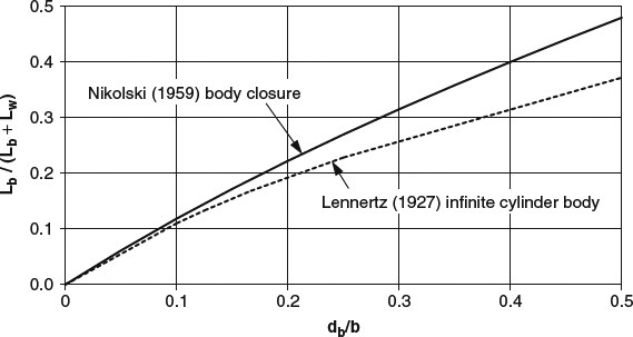
Figure 8.3.15 Comparison of fuselage carry-through lift predicted by Nikolski's (1959) theory for the effect of fuselage closure and Lennertz's (1927) theory that represents the fuselage as an infinite cylinder

For the ideal case, the induced drag is given by

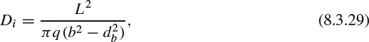
where d_b is the body diameter. Comparing this with Equations 8.3.13 and 8.3.14, we see that it corresponds to an induced-drag efficiency factor given by

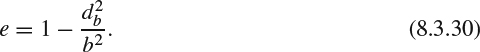
8.3.11 Effects of a Canard or Aft Tail on Induced Drag

True flying-wing airplanes are relatively rare. At least two lifting surfaces, with some longitudinal distance between them, make it much easier to satisfy requirements for longitudinal trim (zero pitching moment) and longitudinal static stability (the tendency to return to the trimmed condition after a disturbance). Thus most airplanes are configured with a main wing and a smaller auxiliary lifting surface, either a forward canard, or, more commonly, an aft horizontal tail (stabilizer). And thus the question arises how the lift loads on these additional surfaces affect the induced drag.

First, let's look at how the trim and stability requirements affect the lift loads the auxiliary surfaces must carry. Longitudinal static stability depends on how the aerodynamic pitching-moment of a configuration changes with angle of attack, which is determined primarily by the planforms and positions of the lifting surfaces and to a lesser degree by the fuselage and engine nacelles. Of course, it is the moment about the center of mass, or center of gravity (CG), that matters, so the other important factor in longitudinal stability is the location of the CG relative to the aerodynamic configuration. The requirement for positive longitudinal stability generally places an aft limit on the CG location, while the requirement to be able to trim the airplane over a range of angles of attack without exceeding the maximum-lift capability of either surface generally defines a forward limit. So stability and trim together define a usable range of CG locations. Within the usable CG range, trimming the airplane for a particular total lift coefficient will require a particular division of the lift between the two lifting surfaces.

For a canard configuration to be stable, the CG must generally be so far forward that the canard must lift upward to trim the airplane at a positive total lift coefficient, and thus trimmer is an alternative name for a canard surface. The lift on an aft tail can be in either direction, depending on how far aft the CG is located. The relatively large horizontal tails of some free-flight model airplanes provide ample stability with the CG far aft, so that an upward load on the tail is required for trim. Most full-sized airplanes have relatively small tails and farther forward CG locations, so that the tail must carry a downward load. Of course, the down load must be offset by increased lift on the main wing.

Proponents often argue that the canard configuration is superior because it is better to have both surfaces lifting up than to have one lifting up and one lifting down, but if we look just at induced drag, we find no support for this argument. For example, consider the simplest idealized comparison we can make:

1. The total lift on the airplane is fixed,
2. The lifting surfaces are coplanar, so that the total induced drag of each configuration is the same as if the total spanload acted on a single lifting surface, and
3. The canard and aft tail to be compared have the same span and carry the same spanload, just of opposite signs, and the loadings on the main wings have the same offset from the elliptic ideal, also of opposite signs, as illustrated in Figure 8.3.16.

The ideal wing alone with an elliptic loading has the minimum induced drag. The total spanloads for the aft-tail and canard configurations represent the same perturbation from the ideal, just in opposite directions. If we represent the total spanloads by the sin series of Section 8.3.8, Equation 8.3.20, both must have the same coefficient A₁ because the total lift is the same. For lateral symmetry, only the odd-numbered coefficients are nonzero, and the deviations of the spanloads from elliptic are thus represented by odd A_i's for i ≥ 3. Because the deviations are of opposite sign, corresponding A_i's are of opposite sign, and according to Equation 8.3.25 the total induced drag is the same. Here I've glossed over the difficulty the sin series would have in representing the kink in the total spanload at the tail or canard tip, but the conclusion is probably still valid.

The above argument indicates no fundamental advantage of a canard over an aft tail in terms of induced drag. But it overlooks some significant practical issues. First, the uploads on canards are typically much larger than the downloads on aft tails. And an elliptic-looking loading on the main wing would be difficult to achieve in the presence of the downwash from a coplanar canard. Besides, it would be better to allow the downwash from the canard to depress the loading on the inboard part of the main wing, and thus to produce a total load closer to elliptic. Another issue is that many real-world configurations are not coplanar, that is there is often a vertical gap between the lifting surfaces.

A nonzero vertical gap between the lifting surfaces has a significant effect on their combined induced drag. How the total induced drag varies as a function of gap depends on how the spanloads on the two surfaces vary. For a look at the gap effect, there are several options regarding the spanloads:

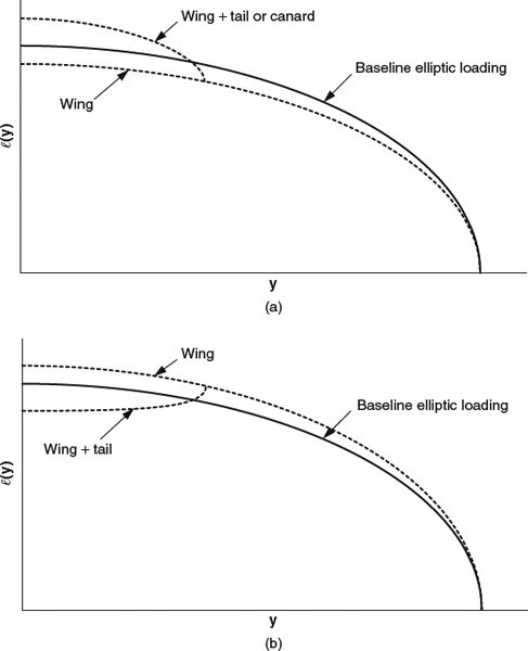
Figure 8.3.16 Illustration of the simple argument for the induced-drag equivalence of a canard and an aft tail. (a) Uploaded tail or canard. (b) Downloaded tail

1. Assume some arbitrary, fixed spanloads, say elliptic on both surfaces,
2. Assume fixed planforms and twist and camber distributions for the surfaces and solve a lifting-surface analysis problem for the spanloads that go with them, or
3. Optimize the loadings on both surfaces for minimum drag, with a constraint on total lift and on either the percentages of the lift carried by the two surfaces or on the total pitching moment, for whatever gap is chosen.

Fixed geometry (option 2) is no longer very relevant to modern design practice. Optimized loadings (option 3) are the most interesting, and we'll compare them with imposed elliptic loadings (option 1) for theoretical interest.

Figure 8.3.17 Variation of induced drag with vertical gap for aft tails or canards with optimized spanloads with a constraint on the percentages of the total lift carried by the two surfaces. Results for elliptic loadings imposed on both surfaces are shown for comparison. Tail or canard span is 0.40b in all cases

Figure 8.3.17 shows Trefftz-plane induced drag as a function of vertical gap for cases in which the second lifting surface has 40% of the span of the wing. In one, the small surface carries a down load equal to 10% of the total lift, as might be the case with an aft tail. The other two cases are up loads of 10% and 30% of the total, spanning a range that might apply to a canard. The basis of comparison D_{i elliptic} is the ideal induced drag of a planar wing carrying the same total lift, with no load on another surface. The calculations are based on Trefftz-plane theory and were carried out in the Boeing WINGOP code (Craig and McLean, 1988). We can make the following observations:

1. For gap ratios greater than 0.2–0.3, there is practically no difference in drag between elliptic loadings and optimized loadings.
2. At the large-gap end, the drag approaches the limiting the case of infinite gap, or two surfaces flying in isolation, for which the optimum is to have each surface carry an elliptic loading; and the total induced drag is just the sum of the two ideal induced drags. These limits are indicated by horizontal lines to the right in Figure 8.3.17.
3. At zero gap, the optimized drag goes to an idealized limiting case in which the total loading is elliptic, and the total induced drag is just the ideal induced drag of a planar wing. The spanload on the canard or tail is not uniquely defined in this case; it has only to satisfy the assumed total canard or tail load required for trim. Then whatever the spanload on the canard or tail is, the wing must carry a load distribution that compensates for it, so that the total load is elliptic. This is an ideal that is not practically realizable, especially if the canard or tail has a spanload with infinite slope at its tip, as is usually true for all practical purposes. Imagine an elliptically loaded canard that sheds the usual vortex wake with concentrated vorticity outboard that rolls up. The wing would somehow have to capture that vorticity and cancel it in order to leave behind a wake equivalent to that of an elliptically loaded wing alone. So the limiting case of zero gap gives us a well-defined theoretical value for the drag, just not a practically realizable one.
4. The 0.1 and −0.1 loading cases with elliptic spanloads go to the same drag level at zero gap, somewhat above the ideal, consistent with our earlier argument that they should differ from ideal by the same amount.
5. For gap ratios less than about 0.2, there is an advantage to optimizing the spanloads, relative to elliptic, but it is small for the smaller tail or canard loadings. Shortly we'll compare the optimum and elliptic spanloads for the small-download case indicated by the diamond symbol, typical of many aft-tail configurations, where the predicted advantage of optimization is only a couple of percent. For large canard loadings, a very small gap is predicted to be good, if the loadings are optimized, and the predicted advantage for optimization is large. But remember that the zero-gap optimum requires the aft surface to “capture” and cancel the vorticity from the forward surface. In this case, only a fraction of the advantage of optimization is probably realizable.
6. Having a second surface of small span carry part of the load can reduce the induced drag only if the load on the second surface is small and upward, and the vertical gap is larger than about 0.2. Most practical, stable canards are probably closer to the 30% load case shown, for which the second surface exacts a sizeable penalty in induced drag unless the vertical gap is very large.

Note that according to Munk's stagger theorem these results are independent of the longitudinal positions of the lifting surfaces. Also note that they should be taken only as indicating qualitative trends, given that they ignore the effects of rollup of the forward surface's vortex wake.

It is interesting to note that for an aft-tail configuration with a vertical gap typical of a large low-wing airplane, the spanload on the wing that gives minimum total induced drag is significantly altered from elliptic. This effect is illustrated in Figure 8.3.18 for a vertical gap of 8% of wingspan (the case indicated by the diamond symbol in Figure 8.3.17). For comparison with the optimum spanload, an elliptic spanload and the optimum spanload for the idealized case of zero gap, assuming elliptic spanload on the tail, are shown. The calculated Trefftz-plane optimum for the spanload on the wing is a kind of washed-out compromise between these limiting cases. Note that on the tail there is very little difference between the optimum spanload and elliptical. Also recall from Figure 8.3.17 that the difference in drag between the optimum and elliptic spanloads is small.

In some treatments of this topic, the induced drag of a two-surface configuration is decomposed into four pieces. Because the downwash experienced by either surface is a first-order quantity, it can be decomposed into a “self-induced” contribution from the same surface and a contribution “induced” by the other surface. The total induced drag can therefore be expressed as the sum of two “self-induced” parts and two parts “induced” on one surface by the other. This approach was convenient in the old days when simplified assumptions were often used in estimating the “shared” parts. Now that numerical Trefftz-plane calculations are so easy to do on a computer, it is just as easy to skip the decomposition and calculate the total drag using Equation 8.3.10. However, there is some intuitive appeal to thinking of the drag in terms of its separate parts. For example, for a downloaded aft tail flying in the downwash from the wing, the contribution “induced” by the wing on the tail is a small thrust that offsets some of the “self-induced” parts of the drag.

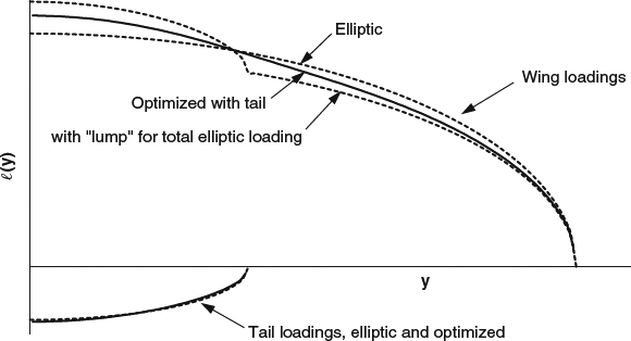
Figure 8.3.18 Optimum spanloads for a wing and a tail or canard with 40% span ratio and 8% vertical gap and downward load equal to 10% of the total lift. An elliptic loading on the wing and an optimum loading for zero gap (an elliptic loading with a “lump” in the middle, so as to have an elliptic total loading) are shown for comparison. The wing spanloads all include an excess over the total lift, to make up for the download on the tail

8.3.12 Biplane Drag

For a given span and total lift, a biplane with some vertical gap between the wings has lower ideal induced drag than a monoplane, according to Trefftz-plane calculations by Munk and Prandtl (see Thwaites, 1958). Their calculations covered a range of span ratios between the two elements of the biplane, but here we'll look just at the case where the two elements are of equal span. In that case, the ideal spanload is the same for both elements, with each carrying half the total lift, and the ideal induced drag depends on the vertical gap as shown in Figure 8.3.19. Note the substantial drag reductions for relatively small gaps, 17% drag reduction for a 10% gap, for example. Also note that the curve is headed for an asymptote at 50% drag reduction as the gap goes to infinity. In this large-gap limit, we have two elliptically loaded wings that don't significantly interfere with each other, each carrying half the lift and a quarter of the induced drag of the monoplane, for a total of half the induced drag of the monoplane.

Given this induced-drag advantage of a biplane over a monoplane of the same span, why aren't more airplanes configured as biplanes? The reasons are several. The biplane arrangement generally incurs higher profile drag and manufacturing cost. Structural weight can either favor a biplane or penalize it, depending on the structural arrangement. If a biplane is configured with the same span and wing area as a monoplane, the biplane wings would have only half the chord of the monoplane, and for the same airfoil thickness ratio would have only half the physical thickness. The smaller thickness would entail a large structural weight penalty unless external bracing (struts and wires) were used. Of course most actual biplanes use external bracing, saving considerable structural weight but incurring a substantial viscous-drag penalty.

Figure 8.3.19 Ideal induced drag of a biplane of equal spans as a function of vertical gap, relative to the induced drag of an elliptically loaded monoplane of the same span. (Calculated by Munk and Prandtl, from Thwaites, 1958)

In the early days of aviation, the preference for biplanes was largely driven by structural weight, as influenced by the airfoil technology of the time. Most of the airfoil data that were available early on were taken in wind tunnels like those built by the Wright brothers, in which models were very small and chord Reynolds numbers were very low. Data at very low Reynolds numbers generally indicate a heavy drag penalty for airfoil thickness, and early designers therefore assumed that airfoils should be quite thin, which favored the externally braced biplane arrangement.

Apart from the drag of struts and wires, the airfoil profile drag of a biplane is an interesting issue and is the subject of some popular misconceptions. When two airfoils are placed in vertical proximity, there is a 2D inviscid interference effect that reduces the lift at a given angle of attack, compared with that of the isolated airfoils. When there is no longitudinal stagger between the wings, this is partly a local-q effect, similar to the one we assumed in our simple model for 2D ground effect in Equation 7.4.2, and partly an induced-camber effect. Some commentators (Garrison, 2008, for example) infer from this lift loss a serious loss in sectional “efficiency” for biplanes. However, inferring an “efficiency” loss from the inviscid lift loss seriously overstates the case. It's true that the lift loss implies a substantial reduction in sectional L/D at fixed angle of attack, but the full reduction needn't be accepted because the lift loss is easily compensated by an increase in angle of attack. And presumably we could even compensate for the details of the induced-camber effect by redesigning the airfoils to produce something close to the same pressure distribution as an isolated airfoil, at least at one operating condition. What cannot be compensated without thinning the airfoils is the induced thickness effect, that is, the effective thickness of the airfoils is increased by their proximity. Indeed, when the viscous drag polar of a biplane pair of airfoils is calculated, the drag is shifted upward by a modest amount relative to the isolated case at the same chord Reynolds number, consistent with an increased effective thickness. The actual loss in maximum sectional L/D is not nearly as gross an effect as that implied by the lift loss at constant angle of attack. In practical design applications, chord Reynolds number is also an issue. A biplane will usually have smaller chords than a comparable monoplane, and the lower Reynolds number will incur some increase in profile drag.

8.4 Wingtip Devices

The idea of a beneficial wingtip appendage or “device” has been around since the early twentieth century, when theoretical calculations first indicated that a vertical endplate added to a wingtip would reduce the induced drag. Early on, however, reality did not live up to the theoretical promise. The simple flat endplate turned out to be a disappointment in practice because the added viscous profile drag more than offsets the saving in induced drag, and the device fails to produce a net benefit. Whitcomb (1976) seems to have been the first to recognize that it is possible to reap the induced-drag benefit of an endplate, and at the same time to realize a net benefit, by keeping the additional profile drag to a minimum through good aerodynamic design practice. The direct result of Whitcomb's work is the classic near-vertical winglet. Less directly, Whitcomb's paradigm of applying good design practice has also contributed to the development of concepts other than the winglet. Both winglets and tapered horizontal span extensions (raked tips) have been put into commercial service, and several other device concepts have also been proposed and brought to varying levels of development (see Figure 8.4.1).

From an aerodynamicist's point of view, the motivation behind all wingtip devices is to reduce induced drag. Beyond that, as Whitcomb showed, the designer's job is to configure the device so as to minimize the offsetting penalties, so that a net performance improvement is realized. For any particular airplane and tip device, the performance-improvement can be measured relative to the same airplane with no tip device.

In Section 6.1.3, we noted that it is not possible to decompose the drag exactly into component parts, but that with the help of idealized theoretical models, it is possible to estimate an induced-drag component. In Sections 8.1 and 8.3, we discussed the physics and the theory of induced drag, including a correct understanding of the role of the vortex wake. Because the vortex wake has been the source of so much confusion regarding how wingtip devices work, we'll take the time to set the record straight on that score before proceeding.

8.4.1 Myths Regarding the Vortex Wake, and Some Questionable Ideas for Wingtip Devices

With our background so far, we are ready to discuss two common misunderstandings regarding the nature and role of the vortex wake. I'll refer to these as the “compactness myth” and the “induction myth,” and after defining them and explaining where they go wrong, I'll discuss some of the erroneous tip-device ideas that arise from them.

The compactness myth is simply the idea that the vortex wake consists of vortex cores that spring from the wingtips and are quite compact from the start. Illustrations that present misleading views of the vortex wake, such as the one in Figure 8.4.2, are common, and they have helped to perpetuate the myth. The water-vapor condensation trails that can sometimes be seen streaming from flap edges or wingtips under humid conditions can also be misleading. These trails tend to mark only an inner portion of the core and give the impression that the core is more compact than it really is. The correct view, as we saw in Figure 8.1.4, is that the vortex wake starts as a sheet and that the wake rollup process generally produces cores that are relatively diffuse. A very compact vortex would require shedding all of the vorticity from the tip itself, which would in turn require a uniform spanload. A uniform spanload simply can't be generated by a wing of any reasonable shape, given the strong downwash that such a loading would entail near the tips. The compactness myth is a simple misunderstanding that by itself wouldn't cause much harm, but when it is combined with the induction myth, the potential for serious mischief arises.

Figure 8.4.1 An assortment of wingtip-device concepts. (a) Raked tip. (b) Blended winglet. (c) 747-400 canted winglet. (d) C-17 canted winglet. (e) MD-11 style up/down winglet. (f) MD-12 style up/down winglet. (g) API spiroid. Used with permission of Aviation Partners, Inc. (h) Tip feathers. (i) Tip fence

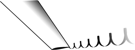
Figure 8.4.2 A misleading view of a compact “wingtip vortex.” From Larson, (2001), drawn by John MacNeill. Used with permission

The induction myth is more complicated and involves a serious misunderstanding of cause and effect. The trailing vortex sheet and the rolled-up vortex cores are often seen as the direct cause of the velocities everywhere else in the flowfield and thus also the cause of induced drag, but this view is mistaken. It is true that when a 3D wing produces its characteristic large-scale flow pattern, as illustrated in Figure 8.1.2, there must be a vortex sheet shed from the trailing edge, but the vortex sheet is not a direct physical cause of the large-scale flow; it is more of a manifestation. The induction myth reflects a common misunderstanding of what the Biot-Savart law represents, a misunderstanding we discussed in Section 3.3.9.

So what kind of mischief can result from the combined compactness and induction myths? The induction myth leads us to think of induced drag as being “caused” by the vortex wake, and thus to think that by doing something very local to change the flow in the core of the “tip vortex” we can have a large effect on the induced drag. To compound the error, the compactness myth leads us to think we can influence the induced drag by acting just on a very small part of the flow. This kind of thinking has spawned many questionable ideas for novel wingtip devices. A common theme is to provide an inlet that swallows the tip vortex itself, or some of the flow that would otherwise become part of the vortex, and to exhaust it straight back, presumably with its swirl and thus its vorticity removed. A schematic illustration of a device of this kind is shown in Figure 8.4.3. Specific proposed devices based on similar ideas are subjects of U.S. patents by Loerke (1937), Frakes (1984), and Hugues (2005). A naive view might lead one to expect such a device to produce dramatic reductions in the strength of the tip vortex and in the induced drag. However, there is no reason to expect that any such device can provide a reduction in induced drag beyond what can be explained as the result of an increase in physical span when the device is added.

The device concept of Figure 8.4.3 has a fatal flaw. It is based on thinking that we can alter the global flow pattern of Figure 8.1.2 by tinkering with the tip vortex, without having to change the overall distribution of lift on the wing. This is wrong, of course. First, we shouldn't expect to be able to alter the general velocity field remotely through the vorticity in a limited region, because as I argued in Section 3.3.9, the vorticity at one point does not directly “induce” velocity elsewhere. Second, unless the overall distribution of lift on the wing is changed, the global flow pattern cannot be significantly altered.

But how can this be? If Biot-Savart is correct, and a device like that shown in Figure 8.4.3 succeeds in swallowing part of the vortex and “straightening” it out, why isn't the global flow pattern changed? The answer is that a relatively small device can only rearrange the vorticity locally; it cannot significantly change the total vorticity flux, as measured, say, by the circulation around each half of the vortex wake. Generally speaking, in this kind of device it is kinematically impossible to eliminate the vorticity flux from a streamtube without producing a compensating vorticity flux adjacent to it.

Let's look at this in a little more detail. Consider a device that swallows an entire vortex into an inlet. Ahead of the inlet, the vortex retains its full vorticity flux and circulation. Inside the duct however, the circulation of the entire captured streamtube must be zero, even before the flow has gone through any straightener. This follows from the no-slip condition on the duct wall. The vortex's original vorticity can still be there in the middle of the duct, but its net vorticity flux is exactly canceled by the net vorticity flux that has been automatically generated in the duct-wall boundary layer. This process involves dynamics, of course, but the net vorticity flux cancelation is a kinematic necessity arising from the no-slip condition. So the internal flow ahead of any straightener contains a vortex in the middle and an equal net vorticity flux of opposite sign in the wall boundary layer. An internal flow straightener could now, in principle, zero out all of this internal vorticity locally, but the net internal vorticity flux was already zero ahead of the straightener. Now consider the flow outside the device. On any closed contour outside the device's external boundary layer, we should see a circulation approximately the same as that of the original vortex. The net vorticity flux associated with this circulation has been automatically generated in the external boundary layer, also by kinematic necessity. Finally, when all of this rearranged vorticity, both internal and external, is shed into the wake, the circulation of the wake and the large-scale flow field outside it will not have been greatly changed, and there will have been no dramatic reduction in induced drag. This is similar to what we noted in Section 6.1.10, that it is impossible for a propeller to produce a net axial vorticity in its slipstream.

Figure 8.4.3 Schematic plan view illustrating a class of tip device that cannot work as intended

8.4.2 The Facts of Life Regarding Induced Drag and Induced-Drag Reduction

We have seen that induced drag is a result of large-scale air motion produced by the lifting system. This motion is not physically “induced” by the vortex wake, but is a response to the lift force and depends on the overall lift distribution. When we try to go beyond this on an intuitive level, we are limited to very general observations, such as that increasing the span of a wing generally reduces induced drag. For anything more specific, especially regarding any device other than a simple span extension, we must rely on quantitative predictions, usually from Trefftz-plane theory. Unfortunately, as we noted in Section 8.3.4, the theory does not generally provide for a simple intuitive understanding of how the details of a particular configuration or lift distribution will affect the drag.

Based on our general appreciation of the physics, we can anticipate that drag-reduction devices need to be fairly large as viewed in the Trefftz plane, because any significant reduction in induced drag requires changing the global flowfield associated with the lift, so as to reduce its total kinetic energy. We know that we can't do this just by tinkering with the “tip vortex” and thus that having a significant effect on the drag requires a significant change in the way the lift is distributed spatially. If our starting point is a wing on which the lift is already advantageously distributed, the only way to improve will be to provide a significant increase in the horizontal span or to introduce a nonplanar element that has a similar effect. The quantitative theory tells us that the effect on drag will be roughly proportional to the horizontal and/or vertical span of the device and that a small device can therefore produce at most a small drag reduction.

There is a common misunderstanding that a wingtip device reduces drag by producing thrust on the surfaces of the device itself. For example, there is the popular explanation that likens a winglet to a sailboat beating into the wind, usually accompanied by a diagram showing the lift vector on the winglet tilted forward by the strong sidewash directed inboard above the wingtip, as in Figure 8.4.4. A corollary is that drag-reduction effectiveness is enhanced if the winglet is mounted well aft on the wingtip, where the sidewash is stronger. This general picture of winglet effectiveness has been put forward by Hackett (1980) and McCormick (1995), among others. It is intuitively appealing, but it is flawed.

First, the idea that there is a favorable sidewash at the winglet location is based on the flowfield (sidewash) that would be there in the absence of the winglet. This view is valid only in the limit of small loading on the winglet and is not even close to being correct for practical levels of winglet loading. When a winglet is advantageously loaded, the flowfield is altered considerably, and the resulting force on the winglet can be very different from what the undisturbed flowfield would lead you to expect. For example, when a wing and vertical winglet are unswept and are carrying their ideal spanload, the sidewash all along the span of the winglet is canceled, and the winglet itself feels no induced thrust or drag. This is required by Munk's minimum-induced-drag criterion from Section 8.3.5, which tells us that any vertical portion of an optimally loaded system must see zero sidewash in the Trefftz plane. With no sweep, the sidewash at the lifting line itself is half what it is in the Trefftz plane, and is therefore still zero on a vertical winglet. So in this case, all of the drag reduction due to the winglet is felt on the horizontal wing, and the sailboat analogy misses the mark badly.

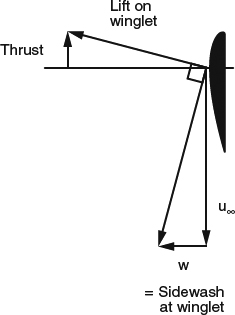
Figure 8.4.4 Misleading view indicating that a winglet produces thrust in the presence of an inboard-directed sidewash “induced” by the wing. Actually, for an unswept wing with a vertical winglet, the optimum loading produces zero sidewash at the winglet only in the limit of small loading on the winglet

So it is a mistake to try to understand a tip device in terms of the flowfield that would be there in the absence of the device, and it is also a mistake to expect the benefit of a tip device to come just from thrust on the device itself. As we saw above, in an optimally loaded unswept wing/winglet combination, the winglet produces no thrust. And the idea of a winglet as a thrust producer fares even worse in the case of a forward-swept wing: An optimally loaded winglet on a forward-swept wing can produce a large drag on its own surfaces and still produce a net drag reduction. In general, the sweep of the wing has a strong effect on the thrust or drag felt by a tip device. Let's look at this sweep effect in more detail.

According to Trefftz-plane theory, the total induced drag of a wing/winglet combination depends only on the arrangement of the trailing edges as viewed in the Trefftz plane and on the spanload (Section 8.3.4). Trefftz-plane theory is not exact, but for high-aspect-ratio surfaces it is a reasonable approximation. Total induced drag should thus be largely independent of sweep, provided that the spanload is fixed. On the other hand, the induced drag or thrust felt by the winglet itself depends strongly on the general sweep of the whole lifting system. In fact, the distribution of induced drag on the whole system, whether it has a tip device or not, is strongly affected by sweep. Induced-drag distributions that illustrate this are shown in Figure 8.4.5. Ideal spanloadings were assumed for a planar wing and for a wing with 20%-semispan vertical winglets, as shown in Figure 8.3.7. The Boeing WINGOP code (Craig and McLean, 1988) was used to carry out numerical lifting-line calculations of the induced-drag distributions for cases in which the wing and winglet are both unswept, and for cases in which both are swept back by 30°, and swept forward by 30°. Small spikes in the distributions at tips are due to the lifting-line numerics, and larger spikes at the winglet junction reflect shortcomings of lifting-line theory (Getting rid of the spikes at the winglet junction would require spreading the bound vorticity out chordwise, as in a lifting-surface theory). In spite of these anomalies, the general trends can be discerned.

In the unswept baseline case (Figure 8.4.5a), the induced-drag distribution is elliptic, as expected. In the unswept winglet case, the drag distribution on the wing is as we might expect based on the spanload in Figure 8.3.7, and the induced drag on the winglet is effectively zero, as we expect based on the theoretical discussion of Section 8.3.5. The strongest reduction in induced drag comes from the inboard part of the wing, and there is a small portion of the wing near the junction where the induced drag is increased.

In the swept cases (Figure 8.4.5b,c), the distributions are dramatically different. For aft sweep without a winglet, there is a large thrust on the outboard half of the wing, more than offset by the large drag on the inboard half. The total induced drag, which is the same as in the baseline unswept case, is a small difference between the two. In the aft-swept winglet case, there is a large thrust on the winglet, which is mostly offset by a reduction in thrust on the outboard wing. The drag reduction on the inboard wing isn't as large as in the unswept case. So in the aft-swept case, there is significant thrust on the winglet, but looking just at that thrust would lead you to grossly overestimate the benefit.

Figure 8.4.5 Induced-drag distributions calculated by numerical lifting-line theory, assuming the ideal spanloadings for a planar wing and a wing with 20%-semispan winglets, as shown in Figure 8.3.7. Lift equivalent to AR = 10.0, C_l = 1.0. (a) Wing and winglet both unswept. (b) Wing and winglet both swept 30° aft. (c) Wing and winglet both swept 30° forward

With forward sweep, we see generally the opposite of what we saw with aft sweep, except that the crossover from thrust to drag is farther inboard. Without a winglet, there is a very large thrust inboard of 10% semispan, more than offset by high drag on the rest of the wing. When a winglet is added, it carries a high drag on its own surfaces, which is more than offset by a reduction in drag over most of the span of the wing. In this case, the sailboat analogy, or any idea of the winglet as a thrust producer, is highly inappropriate.

Trefftz-plane theory tells us that we can reduce the ideal induced drag by increasing the vertical height of the lifting system, as well as by increasing the horizontal span. A vertical fin or winglet that adds vertical height to the system will reduce the ideal induced drag if it is placed anywhere along the span of the wing off of the airplane center plane, but it is most effective by far when it is placed at the station of maximum span; that is, at the tip. This is one example of the more general problem of minimizing the ideal induced drag of a lifting system with given maximum horizontal span and vertical height; that is, a system that must fit within a given rectangular box in the Trefftz plane. Figure 8.4.6 illustrates a series of such configurations, in order from lowest ideal induced drag to highest. The configuration with the lowest drag is the box wing, which has lifting surfaces along all four edges of the box. Note that any retreat from either the corners or the edges of the box (e.g., a “blending” region in the junction between a winglet and the wing in the third example, or the retreat from the outer edge of the box by the “feathers” in the fourth example) increases ideal induced drag, but that there may be compensating advantages such as avoiding the viscous-drag penalty associated with sharp-cornered intersections or reducing the wetted area of the surfaces.

Ideal-induced-drag theory is useful for guidance as to how to achieve a large reduction in induced drag, but the benefits that it implies are not generally achievable in practice. First, the induced-drag reduction that can actually be achieved in most applications typically falls significantly short of ideal. In addition, the actual induced-drag reduction is always offset by other factors that detract from the net benefit to the airplane.

Several factors can contribute to the shortfall in induced-drag reduction relative to ideal:

• Spanloads compromised to save weight: As we discussed in Sections 8.3.5 and 8.3.8, spanloads of real wings are usually compromised to reduce bending loads and save structural weight, by carrying more load inboard and less load outboard than the ideal spanload. (This is in addition to the fact that the spanload with minimum induced drag for a wing in the presence of a down-loaded horizontal tail typically already has less-than-elliptic outboard loading, as we saw in Figure 8.3.18.) If the baseline wing without a tip device and the wing with a device added are both optimized to the same weight/drag objective, they will both carry reduced loads outboard compared with their respective ideal loadings, and a tip device of a given size will have less leverage in reducing induced drag than it would if both configurations had ideal loadings.
• Twist distribution of the existing wing in retrofit applications: If the tip device is to be retrofitted to an existing wing, the jig-twist distribution of the existing wing is nearly always preserved for cost reasons, and as a result the best spanload that can be achieved with the device installed will be farther from ideal than the load on the original wing was. This penalty for keeping the existing twist distribution is larger when the baseline wing is more lightly loaded outboard than ideal, which is usually the case.

  

  Figure 8.4.6 Lifting-surface configurations constrained to fit within a rectangular box in the Trefftz plane (height equal to 10% of full span), shown in order from the lowest ideal induced drag to the highest

• Aeroelastic effects in retrofit applications: In the case of an aft-swept wing, aeroelastic effects may add to the shortfall in drag reduction. Increasing the outboard loading (using a tip device) tends to increase wing bending at cruise conditions, which on an aft-swept wing washes the wing out, reducing the drag benefit of the tip device compared with what it would have been on a rigid wing. The amount of additional wing washout and the resultant reduction of the induced drag benefit will depend on the flexibility of the wing, on the weight distribution of the airplane (payload and fuel), and on whether the structure is beefed up for the addition of the tip device.
• Trim effects: In the case of an aft-swept wing, adding a tip device that increases the loading outboard will increase the download on the horizontal tail that is required for trim, which in most cases will offset some of the induced-drag reduction and add to the offsetting profile-drag increase.

The addition of a wingtip device generally adds wetted surface area and thereby increases viscous drag, and there may also be junction flows or areas with unfavorable pressure distributions that further increase the viscous drag. The redistribution of the spanload that the device produces can change the shock drag on the rest of the wing, but this effect can go in either direction and is usually not large. In any case, the induced-drag reduction is nearly always partly offset by a net increase in the other drag components.

Any practical device that reduces induced drag generally increases bending moments on the entire wing at the cruise condition and at the critical flight conditions that determine the design of the wing structure. The addition of a wingtip device therefore often requires beefing up the wing structure, which adds weight, over and above the weight of the device itself, and subtracts from the net benefit of the device. This trade between drag reduction and weight increase is discussed further in Section 8.4.5. When a tip device is included in the design of an all-new wing, this structural-weight penalty must generally be paid in full. On an existing airplane, flight testing will sometimes have established that the wing has excess structural margin that can be “used up” by the addition of a tip device. The presence of an existing excess structural margin can thus reduce or even eliminate the required beefing up of the existing structure.

8.4.3 Milestones in the Development of Theory and Practice

Lanchester, the British aeronautical pioneer, had developed a qualitative understanding of the 3D flow around a lifting wing, including the vortex wake, by 1895 (Lanchester, 1907). A quantitative understanding of induced drag was first provided by the Trefftz-plane/lifting-line theory, developed by Prandtl in 1910 (Prandtl and Tietjens, 1934) and elaborated by several others in the following years. Even now, well into the era of CFD, our conceptual understanding of induced drag depends almost entirely on this early theoretical work. The conceptual touchstones include

• Ideal-induced-drag theory, including the elliptic ideal spanload (for minimum induced drag) and the simple formula for predicting the ideal induced drag of a planar wing.
• The prediction that multiple and/or nonplanar lifting surfaces, including endplates, could have lower induced drag than a simple planar wing of the same maximum horizontal span.
• Munk's stagger theorem (see Kroo, 2001), and the general prediction that, for a given Trefftz-plane geometry and spanload, the induced drag is independent of the fore-and-aft disposition of the lifting surfaces.

We've already discussed ideal-induced drag theory and pointed out that it provides a method by which the potential induced-drag-reduction effectiveness of various lifting-surface geometries can be compared fairly. One of the best-known examples of such studies is by Cone (1962), in which he used a physical analog apparatus based on a rheoelectric analogy to “solve” the ideal-induced-drag optimization problem and compare many different Trefftz-plane shapes, a sampling of which is shown in Figure 8.4.7. He found that practically any nonplanar shape that adds vertical height near the tip would reduce ideal induced drag. Results like these provided the basis for the development of many of the tip-device concepts discussed in the next section.

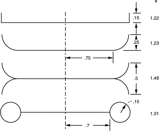
Figure 8.4.7 Some lifting-surface configurations (Trefftz-plane shapes) investigated by Cone (1962). (Published by NASA)

The realization that non-planar lifting systems could generally reduce drag did not immediately lead to successful applications, however. For example, simple flat endplates were tried numerous times in the years after it was first predicted that endplates would reduce induced drag, but in practice they never produced a net drag benefit. Their induced-drag reduction tended to fall short of ideal, and it was always more than offset by the increase in viscous drag due to added wetted area and corner flows. I think it is likely that the failure for so many years to find a better configuration than the flat endplate can be blamed on an “endplate paradigm” based on a particular way of looking at the Trefftz-plane theory. The reasoning leading to the endplate paradigm is as follows. In the limit as the vertical span of an endplate becomes large, the ideal spanload on the horizontal wing becomes uniform. One way to achieve this situation is to have 2D flow over the wing, enforced by endplates that are flat and large in chord as well as span. The resulting paradigm is that an endplate should always be flat and have a large chord.

What the endplate paradigm fails to recognize is that to realize the ideal induced drag of an endplated configuration, only the spanwise distribution of load on the endplate needs to be ideal, and it doesn't matter how the load is distributed longitudinally. A vertical tip device of small chord can achieve the same induced-drag reduction as a large endplate of the same span just by carrying the right spanload. Whitcomb (1976) seems to have been the first to recognize this and to realize that an effective endplate is just another part of the lifting system; that is, a lifting surface that should be carrying a spanload close to ideal, just like the rest of the wing. Of course, to keep the viscous drag of a lifting surface low, the surface should have an efficient aerodynamic cross section; that is, an airfoil, and the chord of the surface should be sized consistent with the efficient load carrying capacity of the section. This is just good aerodynamic design practice of the kind that has always been applied to wings, and Whitcomb's contribution was to apply it to what had formerly been seen as just an endplate. While the direct result of Whitcomb's work was the classic near-vertical winglet, his general idea of applying good design practice to keep the profile drag low has also contributed to the development of concepts other than the winglet.

The trade between drag reduction and structural weight was not addressed explicitly in most early work, but it began to attract attention with the development of the winglet. Whitcomb's work on winglets suggested that for a given increase in bending moment on the inboard wing, a near-vertical winglet offers nearly twice as much drag reduction as a horizontal span extension. This suggestion was not based on theory, but on the results of wind-tunnel tests in which the winglet and horizontal span extension configurations were supposed to be sized so as to be equivalent in terms of root bending moment. However, judging by the results of many later studies, the horizontal span extension Whitcomb used for comparison was not as large as it should have been. Furthermore, the horizontal span extension was not as well optimized aerodynamically as the winglet. Both of these factors contributed to an overly optimistic assessment of the winglet.

Later, a systematic theoretical investigation of the question was published by Jones and Lasinski (1980). They used Trefftz-plane theory to calculate induced drag, and bending moment integrated over the span as an indicator of likely structural weight. (This is only a rough indicator because for real wings at the high-g conditions that are a factor in determining the required structure, the spanload shape is usually different from that at cruise, and the effective structural depth of real wings is not usually constant along the span.) Starting with a baseline elliptically loaded wing of a given span, they added horizontal and vertical tip extensions of varying length. For each device length, they optimized the spanload to minimize induced drag, subject to the constraint that the integrated bending moment, or “structural weight,” was the same as that of the baseline. As the size of the extensions increased, the spanloads had to become increasingly non-ideal (farther from the pure induced-drag optimum) to meet the constraint, and yet drag was still reduced. Repeating the calculations with root bending moment instead of integrated bending moment as the constraint produced essentially the same results. The calculations indicate that horizontal span extensions and vertical winglets offer essentially the same maximum induced-drag reduction when the spanloads are constrained so that there is no increase in “structural weight.” They also indicate that to achieve a given level of drag reduction, a vertical winglet must be nearly twice as large as a horizontal span extension. In Section 8.4.5, we'll see similar results for some variations on the basic vertical winglet.

8.4.4 Wingtip Device Concepts

Whitcomb's breaking of the “endplate paradigm” has led to the development of a variety of wingtip devices that can be effective in reducing total drag, some of which were shown in Figure 8.4.1. It is assumed from here on that Whitcomb's basic idea of applying good aerodynamic design practice will be adhered to in executing any of the concepts. We'll start our discussion of this assortment of competing concepts by listing the basic strategies (Table 8.4.1) that are used in various combinations by the different devices.

Table 8.4.1 Basic strategies for practical tip devices

Increasing horizontal span	Straight tip extensions Tapered tip extensions
Going non-planar	Bending (winglets) Bending with blending (blended winglets: reduced wetted area and junction drag) Splitting (split winglets and feathers: vertical height with less wetted area penalty) Splitting and rejoining (spiroids)
Part-chord devices (less chord than the baseline wingtip)	Trapezoidal baseline tip often has more chord than needed to carry spanload
Pronounced tapering	Reduces wetted area and critical structural loads Applicable to all tip-device concepts
Additional sweep (e.g., raked tips)	Increases aeroelastic washout and reduces wing weight Aeroelastic relief not very effective for a vertical winglet, but sweeping a winglet aft can make transonic tailoring easier

8.4.5 Effectiveness of Various Device Configurations

For comparisons of the potential performance advantages of various tip-device configurations to be fair, the devices in question must be comparably optimized. We've seen that much of the early theoretical work was highly idealized and concentrated on induced drag only. For that case, the appropriate optimization is the minimization of induced drag alone, which defines the “ideal” induced drag and the “ideal” spanload. Ideal-induced-drag theory is useful for initial screening of concepts and for understanding basic trends, and we'll look at such comparisons below, but it is not a realistic optimization target for real-world tip devices. The spanload of a real transport-airplane wing, with or without a tip device, is not generally optimized for minimum induced drag, but instead is optimized for a favorable trade between total drag and structural weight. This is still spanload optimization, just to a bottom-line performance objective such as fuel-burn or maximum range, rather than to an esoteric aerodynamic target.

The usual procedure in design studies is to define the general configuration of a candidate tip device in terms of its planform and dihedral angle(s) and then to estimate its performance through analysis. A step that should always be included in this process is the optimization of the spanload. When the planforms and airfoil cross sections of the wing and the tip device are given, the spanload is controlled by the twist distribution. (Recall that in Section 8.2.1 we defined “twist distribution” to refer to the spanwise distribution of the orientation of the zero-lift lines of the sections. Thus what we refer to here as the “twist distribution” would encompass the overall incidence setting of a tip device, or, for example, the “toed-in” or “toed-out” setting of a winglet, as well as the variation in incidence along the span of the device.) If both the wing and the tip device are all new, the twist distribution of the entire system is open to optimization. In derivative or retrofit applications, the jig twist distribution of the existing wing is generally fixed, and the twist distribution of only the tip device itself can be optimized. If the twist distribution of the existing wing was optimized for operation without a tip device, the benefit available from the addition of the tip device will usually be substantially less than it would have been if the wing could have been reoptimized. In the discussion that follows, it is assumed that the twist distribution of each candidate tip device has been optimized to an appropriate bottom-line performance objective, taking into account structural weight and any other factor that affects the objective, subject to whatever constraints are applicable. For real-world design studies, computational tools are available that can carry out this optimization to different levels of physical fidelity, depending on the purpose of the study.

Device size is always an important design decision, and it affects all devices in essentially the same way. Figure 8.4.8 shows figurative trends in drag, structural weight, and fuel burn as functions of device size for a generic tip device, assuming that the baseline airplane with no device has no excess structural margin, and that for each size the device has been optimized for some bottom-line measure of airplane performance, such as fuel burn. For simplicity, the drag and weight effects are assessed separately first (the drag reduction is plotted for constant weight) and then combined in their overall effect on fuel burn. Note that induced drag cannot be reduced below zero, no matter how large the device is made and that wetted area and profile drag will continue to increase with increasing size. Thus the drag reduction at constant weight must eventually show a diminishing rate of return with increasing size, as indicated by the decreasing slope of the drag reduction curve in the first frame. Because of the ever-increasing profile drag, eventually the drag reduction would reach a maximum and then decline. But for this pure aerodynamic trade at constant weight, the maximum drag reduction would typically occur well outside the practical range of device size. In the real world, the effects of the increasing structural weight would intervene long before that.

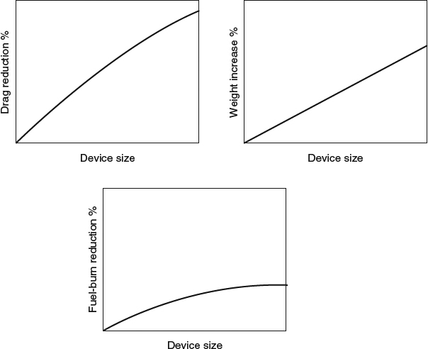
Figure 8.4.8 Effects of device size on performance for a generic wingtip device, assuming no excess structural margin in baseline wing

For reasonable device sizes, the weight increase tends to be roughly linear with size. When the weight increase is taken into account, the fuel-burn reduction generally reaches a maximum well before the maximum in pure aerodynamic drag reduction at constant weight. The optimum device size defined by the maximum fuel-burn reduction depends on the relative importance of drag and weight, which depends on the length of the mission. If maximum range is the objective, the situation is even more complicated because the critical condition that limits maximum range can be different depending on the details of the baseline airplane design. Compared to a device optimized for fuel-burn, a device optimized for range can be anywhere from considerably smaller to considerably larger, depending on the details. Thus the optimum device size depends on many factors, including what performance objective is sought.

Now let's look at the comparative advantages of horizontal span and vertical height. Earlier we mentioned that Whitcomb's work on winglets (Whitcomb, 1976) suggested a rule of thumb to the effect that for a given increase in bending moment on the inboard wing, a near-vertical winglet offers nearly twice as much drag reduction as a horizontal span extension. This rule of thumb has not been borne out by studies since then. Jones and Lasinski (1980) indicated that horizontal span extensions and vertical winglets offer essentially the same maximum induced-drag reduction when the impact on “structural weight” due to bending loads is constrained to be the same.

In Figure 8.4.9, we look at the problem a different way but reach a similar conclusion. While Jones and Lasinski constrained the root bending moment and looked at non-ideal induced drag, here we look at how ideal induced drag is reduced as a function of the increase in root bending moment. In these ideal-induced-drag calculations carried out by the author, induced drag was minimized for a fixed total lift, and root bending moment was free to increase by different amounts for the different devices. The three winglets indicated by the diamond symbols have the same 20% semispan height and thus the same ideal-induced-drag reductions as the corresponding ones shown in Figure 8.4.6. The difference here is that the increase in root bending moment is also shown, on the horizontal axis. Two main conclusions are:

1. For a horizontal span extension to produce the same ideal-induced-drag reduction as a winglet, it needs to be only about half as large (a little more than half compared with a sharp-cornered vertical winglet, and a little less than half compared with a blended or split winglet). A horizontal span extension thus needs less additional wetted area than a winglet for the same induced-drag reduction, and taking profile drag into account would move the total-drag curves for horizontal and vertical devices closer together than the induced-drag curves.
2. For a given increase in root bending moment, the three types of winglets produce roughly the same ideal-induced-drag reduction, about 17% more reduction than a horizontal extension. This is a much smaller difference than the factor of nearly two claimed by Whitcomb (1976). And again, taking profile drag into account makes the total-drag difference even smaller.

Figure 8.4.9 Reduction in ideal induced drag versus increase in root bending moment for the three types of winglets shown in Figure 8.4.6, compared with horizontal span extensions. The lines indicate the trends as the sizes of the devices are increased from zero, and the solid symbols are for two particular sizes that yield roughly comparable drag reductions: 10% semispan horizontal span extensions, and 20% semispan winglets (height measurement)

This comparison is highly idealized and should be taken only as a rough indication of the trends. As we noted above, real tip devices are not generally optimized for ideal induced drag. Also, wing root bending moment associated with the cruise spanload is only a very crude indicator of structural-weight impact. Still, a general conclusion is that horizontal span extensions and vertical winglets have very similar performance potential in terms of the trade between drag reduction and weight increase. In general, in the choice between winglets, horizontal span extensions, and other tip-device configurations, there is no clear-cut favorite for all applications. In terms of the basic physics, the benefits they offer tend to be comparable. Which choice is favored for a particular application depends on the details of the baseline airplane design, both aerodynamic and structural, and on the mission objective. And the differences between the choices are usually not large.

Theoretically, there is a small general advantage for devices in which the lifting surface splits into two branches. In general, splitting allows a given level of induced-drag reduction to be achieved with less additional wetted area than a non-split configuration would require. For a feather configuration with a small included angle (see Figure 8.4.6), the wetted-area increase is only a little more than that of a horizontal span extension of the same projected span, but the induced-drag reduction is considerably greater. Of course, the weight increase is also considerably greater, so that the advantage in terms of drag versus weight is not large. If we increase the included angle between the feathers to 180°, we have split vertical winglets of equal span. Comparing this with a simple vertical winglet of the same total height, we find that the optimum spanloads for both are about the same just inboard of the junction. In the case of the split winglets, this load splits evenly between the two branches, so that if we size the chord of the device according to the load carried, the split winglets need only half as much chord as the single winglet. The split winglets produce about 90% of the induced-drag reduction of the single winglet (compare the “split winglets” with the “vertical winglets” in Figure 8.4.6) with only about half as much additional wetted area. A drawback to split winglets in practice is that the span of the lower winglet is often limited by ground clearance.

8.5 Manifestations of Lift in the Atmosphere at Large

In previous sections, we looked at the flow around a 3D wing, the lift distribution on a 3D wing, and the theory of induced drag. In this section, we look at the manifestations that the lift on a wing has in the atmosphere on a large scale and at some of the theoretical issues that arise in representing those manifestations.

We start with a look at how the flowfield associated with the lift satisfies Newton's laws in an integrated sense. Highly simplified models suffice for this purpose, but the mathematics involved is tricky, and some erroneous results have been widely propagated. A secure understanding of these issues thus requires addressing how the erroneous analyses went wrong. When the smoke has cleared, we'll find that there is no net downward momentum imparted to the atmosphere as a whole and that the lift is reacted by pressure differences on horizontal planes above and below the wing, or on the ground plane, if there is one. We'll also consider how conservation of momentum applies to control volumes that don't encompass the entire atmosphere. To keep things simple, we'll look only at rectangular volumes with horizontal and vertical surfaces. We'll find that the lift can show up at the boundaries either as pressure differences on the horizontal surfaces or as fluxes of vertical momentum mainly through the vertical surfaces, or as combinations of the two, depending on the proportions of the control volume.

Finally, the actual process by which the vortex wake disappears far downstream has received little coverage in the usual aerodynamics sources, and we'll attempt to at least fill in a rough picture of what happens there.

8.5.1 The Net Vertical Momentum Imparted to the Atmosphere

There is a widespread notion that an airplane in steady level flight continuously imparts net downward momentum to the atmosphere. Contributing to this notion is the fact that the airplane is continuously adding to the impulse of its vortex-wake system and the fact that there is net flux of downward momentum across vertical planes behind the airplane, issues we'll deal with in the following sections. We also saw that a 2D airfoil imparts a downward momentum change to the air, but confusing the issue in that case is the fact that the downward momentum behind the airfoil accounts for only half the lift. However, appearances are deceiving, and the notion that the airplane leaves behind a continuously increasing net downward momentum is mistaken.

For our purpose of assessing the net vertical momentum, a very simple model of the flowfield produced by an airplane in steady level flight suffices. That is the classical, highly idealized model in which the vortex wake is represented by a pair of parallel line vortices, and the sinking and any other deformation of the wake are ignored. Assuming the airplane has been flying for a finite time since an impulsive start, we then have a vortex system consisting of a planar, rectangular loop, as shown in Figure 8.5.1. This model is unrealistic in several ways, especially in the vicinity of the starting vortex. Spalart (2008) has pointed out that a simple flow structure for this part of the vortex loop is not sustainable over time, where in the real world the vortex system would quickly distort, become unsteady, and disperse. However, we'll find that the starting vortex isn't a player in the overall vertical-momentum balance, which indicates that this oversimplification does no harm for the level of analysis we're attempting here. And in Section 8.5.5, we'll discuss how the vortex wake really terminates downstream.

Figure 8.5.1 Idealized rectangular-loop model for the vortex system of a 3D wing flying for a finite time

Given our representation of the vortex-wake system as a closed vortex loop, a relevant concept is that of the impulse of a vortex loop. It is known that any incompressible potential flow can be established by the application of an impulsive pressure field at an initial instant, starting from an initial condition in which the fluid is at rest (Milne-Thomson, 1966, Section 3.31). In the case of a closed vortex loop like the one in Figure 8.5.1, in a field that would otherwise be at rest, an impulsive pressure field that could initiate the flow would have to impose a net impulse on the fluid, proportional to the circulation and the area of the loop, and in the direction perpendicular to the plane of the loop (Milne-Thomson, 1966, Section 10.21). This is what is called the impulse of the vortex loop. In our idealized model, the rectangular loop of Figure 8.5.1 is attributed to an airplane flying with lift L for time t. The impulse of this vortex loop, and the actual mechanical impulse imposed by the airplane on the atmosphere (lift times time), are both equal to Lt. They both increase with time as the airplane continues to fly and the area of the vortex loop grows. So we have a one-to-one correspondence between the mechanical impulse imposed by the airplane and the impulse of the vortex loop.

Thinking in intuitive physical terms, we might also expect the impulse imposed by the airplane on the air (the product Lt) to produce a net vertical momentum in the atmosphere that grows with time. This expectation is not satisfied by the mathematics, however. Wigton (1987, private communication) showed that the volume integral of the vertical velocity inferred from the vortex system, over the whole infinite atmosphere, is nonconvergent. The integrand (the vertical velocity) doesn't decrease fast enough with increasing distance (only as r⁻³), and the flowfield associated with the vortex loop thus contains infinite amounts of both upward and downward momentum. An attempt to define a value for the integral can lead to any answer between minus infinity and plus infinity, depending on how the integration is sequenced. Thus the vertical-momentum content of the infinite atmosphere at any given time is at best undetermined, even though the mechanical impulse imposed by the airplane and the impulse of the vortex loop are well defined.

This unsatisfying result is an artifact of our idealized assumptions: incompressible flow and an infinite atmosphere. In the real world, no disturbance generated by the airplane would propagate faster than the speed of sound, and for finite flight time all flowfield integrals would be well defined, so presumably we could resolve this difficulty by doing an unsteady compressible analysis. But there is an easier way. The problem is resolved if we consider flight in a semi-infinite atmosphere bounded by a ground plane. The simplest way to impose the no-through-flow condition at the ground plane is to place an image of the “real” vortex system below the ground, as shown in Figure 8.5.2. This is the same thing we did in Figure 8.2.6 to model flight close to the ground, but this time our purpose is to model flight many wingspans from the ground. At large distances, the velocity disturbances associated with the vortex loop and its image die off as r⁻⁴, which is fast enough for the vertical-momentum integral to converge. If we expected to see a net downward momentum equal to Lt, the result comes as a surprise: The value of the integral over the semi-infinite space above the ground is zero, which means that the airplane imparts no net downward momentum to the atmosphere in steady level flight over a ground plane, regardless of height above the ground. If momentum conservation is to be satisfied, there is only one other way the lift can be balanced, and that is by the pressure, which is our next topic.

8.5.2 The Pressure Far above and below the Airplane

Our finding of zero net vertical momentum shouldn't have been a surprise. Prandtl and Tietjens (1934) showed how in steady level flight the lift is balanced by an overpressure on the ground under the airplane, so that of course there is no need for net momentum transfer. They assumed a rectangular vortex system and its image, like that shown in Figure 8.5.2, and showed that when the height is large compared with the wingspan, there is no significant pressure disturbance at the ground associated with the trailing vortices, but that there is a disturbance at the ground associated with the bound vortex and its image, given by

where h is the airplane's height above the ground and R is the radial distance from the airplane to the point in question on the ground. The disturbance is thus distributed in a pattern of circular isobars centered directly under the airplane. The overpressure dies off radially in a bell-shaped distribution, as shown in Figure 8.5.3, and Prandtl and Tietjens showed that the integrated pressure disturbance accounts for all of the lift. The gross features of the pressure footprint predicted by the simple incompressible model are not altered by compressibility at subsonic speeds. For steady flight, the footprint remains centered under the airplane regardless of the Mach number, as long as it is subsonic. This steady-flow pressure distribution is not like an acoustic radiation pattern, which would lag behind the airplane at high subsonic Mach numbers.

Figure 8.5.2 The rectangular-loop vortex system of Figure 8.5.1 reflected in a ground plane

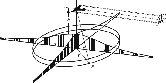
Figure 8.5.3 The airplane's pressure footprint on the ground in steady, level flight. From Prandtl and Tietjens, (1934). Used with permission of Dover Publications, Inc.

The presence of an integrated pressure disturbance imposed by the airplane on the ground plane has an easy intuitive interpretation: The ground plane is supporting the weight of the airplane in addition to the weight of the atmosphere. The typical local magnitude of the pressure disturbance at the ground is extremely small. For example, for a 747 weighing 800 000 pounds flying at 35 000 ft AGL, the maximum pressure disturbance directly under the airplane is 1.0 × 10⁻⁴ pounds per square foot or 5 × 10⁻⁸ atmospheres. And, of course, the area covered by the disturbance is typically quite large. The disturbance is greater than half its maximum value inside a circle on the ground of radius 0.766 h, which for our 747 at 35 000 ft covers an area of 81 square miles.

Above the airplane, the integrated pressure disturbances “due to” the bound vortex and its image cancel each other, which is consistent with having all of the lift accounted for by the pressure disturbance on the ground below. The other place we should look for manifestations of lift is under the starting vortex, which wasn't mentioned by Prandtl and Tietjens and which in the real world would be out of the picture in any reasonable length of time. We'll look at it anyway, just to understand the full implications of our vortex-loop model. One might expect that there would be a “suction” footprint under the starting vortex, a mirror image of the pressure footprint under the airplane, because the starting vortex has a rotation opposite to that of the bound vortex. But it turns out that the integrated pressure disturbance under the starting vortex is zero. This is an instance in which being in the right reference frame is crucial.

The Prandtl and Tietjens analysis of the pressure footprint is carried out in the reference frame moving with the airplane, in which the flow under airplane is steady, and the steady form of Bernoulli's equation holds. In this reference frame, there is a substantial freestream velocity, and far below the airplane, where the disturbances are small, the pressure disturbance goes as ρu_∞u, that is, the pressure disturbance is first order in the velocity disturbance u. To use the steady Bernoulli equation in the analysis of the flow under the starting vortex, we must move to the reference frame of the air mass, in which the starting vortex is not moving. In this frame, there is no freestream velocity, and the pressure disturbance goes as ρu², second order in the disturbance velocity, so that the integrated pressure disturbance vanishes in the limit of large height.

So we see that for steady level flight in a semi-infinite atmosphere the lift is transmitted to the ground by the spread-out pressure disturbance of Figure 8.5.3. And none of the conclusions we've drawn here would change much if we introduced a more realistic model for the flow and the development of the wake near the airplane.

Now let's return briefly to the case of the infinite atmosphere. The Prandtl and Tietjens analysis of the pressure on the ground plane has interesting consequences when it is applied to the situation without a ground plane. If we remove the ground plane by removing the image vortex system, the pressure disturbance at the original location of the ground plane is reduced to half what it was when the ground plane was there. And in the absence of an image vortex system, the integrated pressure disturbance above the airplane is not canceled. So looking at horizontal planes above and below, we now have a positive integrated pressure disturbance below the airplane accounting for half the lift, and a negative disturbance above the airplane accounting for the other half, as illustrated in Figure 8.5.4a. This holds regardless of how far above and below the airplane we place the planes. The transport of vertical momentum through these horizontal planes above and below the airplane is second order in the velocity disturbances, so that its integrated effect vanishes as we move the planes far away. All of this indicates that in an infinite atmosphere, pressure differences on horizontal planes far above and below the airplane account for the lift, and that there is no net transfer of momentum to the atmosphere. This of course implies that the “physically correct” value for the volume integral of the vertical momentum in the atmosphere should be zero, though we found it before to be mathematically indeterminate.

8.5.3 Downwash in the Trefftz Plane and Other Momentum-Conservation Issues

We've seen that no net vertical momentum is imparted to the atmosphere as a whole by an airplane in steady level flight. However, there are regions of both upward and downward momentum in the field, and it is instructive to look at the momentum balance at the boundaries of control volumes that don't encompass the entire atmosphere. We'll limit our attention to rectangular volumes with vertical and horizontal faces and start by considering fluxes of vertical momentum across vertical planes at various stations in the flow. One example is the Trefftz plane downstream of the airplane, which we used as the downstream boundary of a control volume in our derivation of the general farfield integral for the induced drag, Equation 8.3.5. Then, of course, it was the flux of flight-direction momentum we were interested in, while now it is the flux of vertical momentum.

There is a classical argument for the downward momentum at the Trefftz plane in an infinite atmosphere that goes as follows. A rectangular vortex loop is assumed, as in Figure 8.5.1, and the Trefftz plane is placed between the bound and starting vortices, far from both, and is pierced by the trailing vortices. At sufficiently large distances, the bound and starting vortices contribute nothing, and only the trailing vortices have to be considered. The expression for the w disturbance “induced” by a trailing-vortex pair of infinite length is then integrated over the Trefftz plane, and the result is found to be (Thwaites, 1958, p. 303, for example)

Figure 8.5.4 Balancing momentum, pressure, and lift in rectangular control volumes of different proportions. (a) with no ground plane, or with a ground plane far away relative to any dimension of the control volume. (b) with a ground plane as the bottom boundary of the control volume. (c) with or without a ground plane

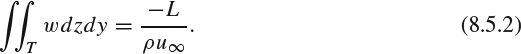
A widely held interpretation of this result is that there is a flux of downward momentum through the Trefftz plane, consistent with the lift on the wing, and that it is “induced” by the trailing vortices.

However, it turns out that this classical result is incorrect. Wigton (1987, private communication) found that the w integral 8.5.2 is nonconvergent (w dies off only as r⁻²), and he observed the classical symptom of nonconvergence, that is, that the value obtained depends on the order of integration. Reversing the order from that shown in Equation 8.5.2 yields a value of zero. Wigton also found that if he used the w expression for trailing vortices of finite length, consistent with a finite vortex loop as in Figure 8.5.1, the integral converges, and the correct answer is zero, regardless of the length of the vortices or the order of integration:

So Wigton concluded that the classical argument is wrong and that the part of the velocity field “induced” by the trailing vortices results in no net flux of vertical momentum through the Trefftz plane. Lissaman (1996) independently came to the same conclusion.

The story of this error represents an interesting cautionary tale. Clearly, incorrectly evaluating an improper integral is an easy trap to fall into. You can apply the standard procedures for evaluating integrals and, without making any procedural error, obtain a wrong answer. Equation 8.5.2 fortuitously gave the “expected” result, which apparently fooled more than one prominent aerodynamicist. And the incorrect result has been used in other analyses, rendering them incorrect as well. Sears's analysis of the pressure in the Trefftz plane is an example we'll discuss in Section 8.5.4.

The trailing-vortex result of Equation 8.5.2 is not the only error Wigton found. He also found that the classical argument that the bound and starting vortices contribute nothing is wrong. For any Trefftz plane between the bound and starting vortices, each “induces” an integrated downward momentum corresponding to half the lift, regardless of distance. At large distances, the w disturbances “induced” by the bound and starting vortices are very small, but are spread over a very large area. Thus the Trefftz plane in an infinite atmosphere does see a flux of downward momentum corresponding to the lift after all, but it is distributed very differently from the way it was in the classical picture, in which it was assumed to be associated with the trailing vortices. Lissaman (1996) also independently found this result. It applies only to a vertical plane between the bound and starting vortices. For a vertical plane either ahead of the airplane or behind the starting vortex, the flux of vertical momentum is zero, because the integrated contributions from the two vortices cancel.

This finding of an integrated downward momentum in some vertical planes and none in others appears to contradict our finding of zero for the volume integral of the vertical momentum, even for an infinite atmosphere (in Sections 8.5.1 and 8.5.2). If we view the infinite-atmosphere case as a series of “Trefftz-plane” slices stacked in the flight direction, we see no net downward momentum in the slices ahead of the airplane or behind the starting vortex, and nonzero net downward momentum in the slices between the airplane and the starting vortex. If we were to naively sum the stack, we would conclude that the atmosphere contains a net downward momentum equal to Lt. But this naive summing is just another example of an incorrect evaluation of an improper integral, in this case the 3D volume integral of w in an infinite domain. Remember that we found that this integral is nonconvergent and therefore indeterminate mathematically. Physically speaking, however, our argument based on the pressure indicated that the airplane imparts no net vertical momentum to the atmosphere. So the physically “correct” value for the volume integral of the vertical momentum in an infinite atmosphere is still zero and is not contradicted by the Trefftz-plane findings.

So how do we reconcile a net flux of downward momentum in the Trefftz plane with the findings that there is no net vertical momentum imparted to the atmosphere by the lift and that the lift is reacted by pressure differences on horizontal planes? If we look at the momentum balance in control volumes of different proportions, as illustrated in Figure 8.5.4, it appears that all of this can be reconciled, though we'll find that the lift is accounted for either by pressure or by momentum flux, depending on the proportions of the control volume.

Consider rectangular control volumes with dimensions Δx, Δy, Δz. Assume that the spanwise dimension Δy is very large compared with the other two, so that fluxes of vertical momentum through the side boundaries effectively vanish. Now, keeping Δx and Δz much smaller than Δy, we can define two limiting shapes for the control volume in side view, tall and slender, or wide and flattened. Looking at these limiting cases with and without a ground plane gives us the three combinations shown in Figure 8.5.4. Unlike Wigton's (1987, private communication) analysis above, we put the starting vortex out of the picture by assuming that it is far downstream relative to any dimension of our control volume, so that its “contribution” to any integrated momentum fluxes effectively vanishes. There are only three distinct combinations in Figure 8.5.4 because, with the starting vortex out of the picture, it doesn't matter whether there is a ground plane in the case of the tall, slender control volume in Figure 8.5.4c. The momentum balances then work out as follows:

1. with no ground plane, or with a ground plane far away relative to any dimension of our control volume, so that the image vortex system has negligible “effect”: As Δx grows large relative to Δz, the integrated fluxes of vertical momentum through the upstream and downstream boundaries effectively vanish, and the lift is accounted for by the pressure disturbances on the top and bottom boundaries, as in Figure 8.5.4a. The pressures on the top and bottom boundaries account for half the lift each, regardless of the relative distances above and below the airplane. If one of the boundaries is moved farther away, the pressure disturbances become weaker but are more spread out, so that the integral is unchanged.
2. with a ground plane as the bottom boundary of the control volume: As in (1) above, the integrated fluxes through the upstream and downstream boundaries effectively vanish, and the lift is accounted for by the pressure disturbance on the ground, as in Figure 8.5.4b. This is similar to what we found in Figure 8.5.4a, except that the ground plane has the effect of doubling the pressure disturbance there, so that it accounts for all of the lift, and the pressure footprint is the same one illustrated in Figure 8.5.3. On the upper boundary, the disturbances “due to” the bound vortex and its image are of opposite signs and cancel in an integrated sense. But they do not cancel locally. There is a central region directly above the airplane where the “contribution” of the bound vortex dominates, and the pressure disturbances are negative. At larger horizontal distances, the “contribution” of the image vortex dominates, and the pressure disturbances are positive. The positive disturbances are much weaker than the negative disturbances, but they can cancel the positive disturbances in the integral sense because they are spread over a much larger area (note that the distribution is axisymmetric, and the integration is therefore radius-weighted).
3. with or without a ground plane: As Δz grows large relative to Δx, the integrated pressure forces on the top and bottom boundaries effectively vanish, and the lift is accounted for by the fluxes of vertical momentum through the upstream and downstream boundaries, as in Figure 8.5.4c. Because we have put the starting vortex out of the picture, the total flux of vertical momentum is split equally between upward momentum upstream and downward momentum downstream instead of showing up only as downward momentum downstream, as it did in Wigton's (1987, private communication) analysis. This is the same distribution of integrated momentum flux that we found in 2D in Section 7.3.4.

I've presented these arguments in an arm-waving way, but I'm confident they represent correct limiting cases. They demonstrate that there is no inherent contradiction in seeing the lift manifested both as pressure disturbances on horizontal planes and as fluxes of vertical momentum through vertical planes. And there is no inconsistency between these manifestations and our earlier finding of no net vertical momentum in the atmosphere.

8.5.4 Sears's Incorrect Analysis of the Integrated Pressure Far Downstream

Sears (1974) used conservation of momentum in control-volume form, combined with the classical Trefftz-plane integral for the induced drag, Equation 8.3.10, to deduce that the integrated pressure in the Trefftz plane behind a lifting wing in inviscid flow is higher than ambient.

On an intuitive level, this result is surprising, because we tend to think of induced drag as being associated with the kinetic energy left behind in the downstream flowfield, and we tend to associate excess kinetic energy with a velocity magnitude higher than freestream, and pressure lower than ambient. We also tend to associate the swirling motion about the vortex cores with lower-than-ambient pressure. But our naive intuition in this case is mistaken. In inviscid incompressible flow, the pressure perturbation goes as −2Uu − u² − v² − w², so that even though v and w tend to be larger in magnitude than u near the vortex wake, the −2Uu term is of higher order and can dominate. When downwash occurs near a tilted wake, u can be negative, and the perturbation pressure can be positive, contrary to our naive intuition. So there can be regions of positive perturbation pressure behind a lifting wing, and we can't rule out Sears's result just on the basis of arm waving and intuition.

But it turns out that Sears's conclusion is actually wrong. Given his flowfield model, there is a region of higher-than-ambient pressure in the Trefftz plane, but the integrated pressure is lower than ambient, not higher. So where did the analysis go wrong?

Figure 8.5.5 Sears's (1974) model using a planar, tilted vortex wake, and Trefftz plane perpendicular to flight direction

Sears assumed that the wing is elliptically loaded and that the vortex wake remains planar but is tilted downward as shown in Figure 8.5.5, at an angle consistent with what this wake model gives for the downwash far downstream of the wing. He assumed that far downstream the velocity disturbances are those “induced” by the vortex wake perpendicular to its own plane, and he substituted these velocity disturbances into the integral expressions governing the integrated momentum balance. The tilt angle of the wake thus enters directly into his analysis, which is unfortunate, as the tilt angle of an undistorted tilted wake is much too large, π²/2 ≈ 4.9 times that of a realistic rolled-up wake, as we saw in our discussion of ideal induced drag in Section 8.3.5.

But even being this far off in the tilt angle of the wake isn't enough to account for the wrong sign in the final result. That, it turns out, is the result of a mathematical error. One of the integrals appearing in Sears's analysis is the integral of w, that is, the integrated down-wash in the Trefftz plane, associated with the trailing vortex wake, for which he assumed the incorrect value from Equation 8.5.2, −L/(ρu_∞). We saw earlier that this integral is nonconvergent for a wake of infinite length, but that its value is zero for a wake of finite length, regardless of the length. Had Sears used the correct value of zero for the w integral, he would have obtained the negative value −D_i for the integrated pressure in the Trefftz plane, instead of the erroneous +D_i, where D_i is the induced drag.

8.5.5 The Real Flowfield Far Downstream of the Airplane

Most of our discussion so far has been based on a vortex-wake system consisting of a rectangular loop terminated at the downstream end by a starting vortex, though we noted that the assumption of a persistent starting vortex is unrealistic. Of course, in the real world, the starting vortex would be left on the runway where the airplane took off, and it would dissipate rapidly through viscous interaction with the ground. And there would be diffuse spanwise vorticity left behind as the bound vorticity changed during climb and the transition to cruise. But even if the flight started impulsively at cruise altitude, the starting vortex could not persist in the simple form we assumed. So what really happens far downstream, as the vortex-wake system collapses and the flow disturbances associated with the lift die out?

For purposes of this discussion, we'll skip the complexities of takeoff and climb. We'll assume the airplane has been in steady level flight at high altitude for a long time, and we'll seek a “steady state” understanding of the flowfield far downstream, in which a starting vortex is no longer in the picture. In Section 8.1, we described some features of the flow, up to the point where the wake “collapsed” into an unsteady pattern of loops and eddies. Here, we'll attempt to deduce what the time-averaged structure of the flow must be throughout this process of collapse and beyond, to where the velocity disturbances die out. The final stages of this progression are not of any practical importance, because the mean velocities become very small. It's just an interesting and informative exercise to figure out what the laws of motion require.

For a long distance downstream of the airplane, the rolled-up vortex wake is relatively compact and retains the descending-oval form shown in Figure 8.1.7, and the velocity and vorticity distributions shown in Figure 8.1.8 change very little. The collapse of the wake starts with the slow growth of instabilities such as the Crow instability, which leads eventually to breakup into loops and eddies, as shown in Figure 8.1.10. This process is highly variable in response to atmospheric conditions, and it changes over short and long time scales. Downstream of breakup, we have a turbulent flow with motions over a wide range of length scales, spread over a much wider area than the original descending oval occupied.

Of course, this breakup into a diffuse turbulent flow doesn't mean the vorticity in the upstream wake has disappeared. Remember that Helmholtz's second theorem tells us that vortex lines can't end in the interior of the field. The vortex lines from the wake upstream haven't ended in the field, but in the instantaneous turbulent flow downstream of breakup they have become an unsteady, chaotic tangle. Does this mean the flow is just an unorganized turbulent jumble that is otherwise featureless? No. Averaged over time, the flow must have an overall structure consistent with its origins upstream. The time-averaged flow must obey all the same kinematic rules as any other flow, which means that the abundant time-averaged vorticity that was present in the wake upstream cannot end in the interior of the field any more than the instantaneous vorticity could. And the time-averaged flow must obey the RANS equations, with the instability motions and turbulence supplying the Reynolds stresses (see Section 3.7) that transport time-averaged momentum.

So to see the underlying structure of what happens during and after breakup, imagine time-averaging the flow in the reference frame moving with the airplane, so as to take out the unsteady motions on the time scales of the instability and the eventual turbulence. This is formally the same process we used in Reynolds averaging for turbulence modeling (Section 3.7), but in this case the flow we're applying it to is different from the more usual applications of Reynolds averaging. For one thing, we'll be averaging out part of the motion (the highly coherent motion associated with instability growth) that doesn't look like ordinary turbulence. And over much of the flowfield far downstream, the mean-velocity disturbances are smaller than the turbulent fluctuations and are effectively invisible before we do the averaging. Furthermore, we'll do this strictly as a thought experiment, since no such calculation has actually been done, to my knowledge. We'll do the averaging in our imaginations and use physical reasoning to try to deduce what the qualitative structure of the time-averaged flow must be.

First, we'll assume that the airplane and the mean flow are symmetrical about the y = 0 plane. We'll also assume that at the start of the instability-growth and breakup process the wake is in the form of a descending oval as in Figure 8.1.7 and that the vorticity is still concentrated in two distinct cores, as in Figure 8.1.8b. The net vorticity and circulation of the core on either side of the symmetry plane must then be the same as what was shed into the nearfield from the corresponding half of the wing. One of the main things we'll be looking to explain is where all this mean-flow vorticity “goes” in the farfield, consistent with the requirement that vortex lines can't end in the interior of the field.

Something we know from observations is that things change slowly in the flight direction. Even though the breakup process produces much faster change than what ordinary turbulent diffusion could produce, change in the mean flow is still slow in the sense that the flight-direction distance over which it takes place is long compared with any other dimension of the wake. Thus we have an effectively “slender” flow in which mean-flow gradients in the direction of the wake axis play a much smaller role in the development of the flow than do gradients in other directions. In this sense, the flow in cross-flow planes is similar to the limiting case of 2D planar unsteady flow, and as an aid to understanding, it is useful to look at what can happen to the mean vorticity in simple 2D cases.

In 2D planar flow, the mean vorticity vector can have only one nonzero component, perpendicular to the plane of the flow, so we can think of the vorticity as a scalar. We'll start with the example of a single axisymmetric vortex core in an infinite 2D domain. At an initial instant, we have some axisymmetric distribution of vorticity, as shown in Figure 8.5.6a, and as time goes on it remains axisymmetric but becomes more diffuse, as in Figure 8.5.6b. The integrated vorticity and circulation remain constant, even as the vorticity spreads over a very large area and becomes locally very weak.

Our second example is a pair of counter-rotating vortices of equal strength separated by a plane of symmetry, like our vortex wake. In this case, each core has its own total vorticity and circulation in its own half of the domain, but because the two cores have vorticity of opposite signs, the total vorticity and circulation of the entire flow are zero. Starting with two cores that are initially distinct, as in Figure 8.5.7a, viscous or turbulent diffusion eventually brings the cores into “contact” in the sense that the vorticity gradient becomes significant across the plane of symmetry, as in Figure 8.5.7b. Because there isn't any no-slip surface anywhere in the field to interact with, vorticity can be destroyed only by interaction with vorticity of opposite sign, and that is what happens here. Vorticity is diffused toward the symmetry plane and annihilated there by interaction with the opposite-sign vorticity on the other side, and the circulation on each side of the symmetry plane is reduced. In this example, not only does the vorticity become more diffuse and locally weaker, but the total vorticity on each side of the symmetry plane tends to zero with time. In this 2D domain, vorticity disappears in time, without having vortex lines end in space, so Helmholtz's second theorem is not violated.

What does this imply for our real 3D flow? As we've already observed, the 3D mean flow throughout the region of breakup and decay is “slender” and therefore behaves in a nearly 2D fashion, but it is steady by definition in the reference frame of the airplane. Imagine cutting this flow with a constant-x plane fixed to the atmosphere, so that in the airplane reference frame, the cutting plane moves away from the airplane at the speed of the freestream. For the flow that we observe in the cutting plane, the movement in x is analogous to the advance of time in the 2D flow we just discussed, and much of what happens will be similar in the two cases. In the 3D case, the vigorous “turbulent” motions of the instability growth will diffuse the mean vorticity in all directions, including toward the plane of symmetry, just like what we saw in 2D in Figure 8.5.7b, only faster. As our cutting plane continues to move downstream, vorticity diffusing toward the symmetry plane will effectively disappear there, and the integrated vorticity passing through the cutting the plane on each side of the symmetry plane will decrease, as it did in the 2D case.

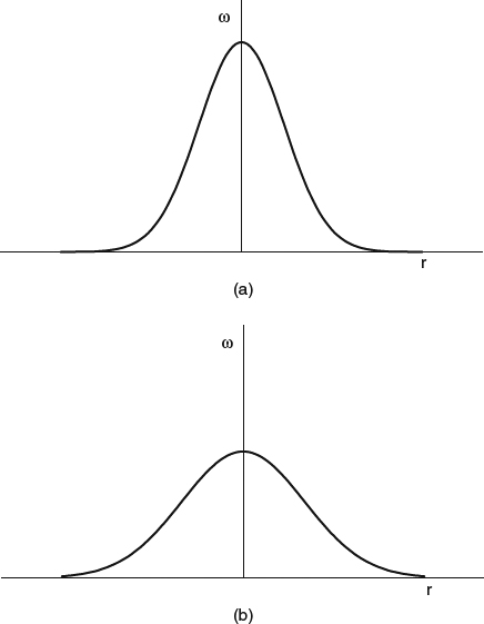
Figure 8.5.6 Diffusion of vorticity in a single axisymmetric vortex core in 2D unsteady flow. (a) at an initial instant. (b) More diffuse at a subsequent time

The analogy between our 3D steady mean flow and the 2D unsteady case isn't perfect, however, and there must be some differences in the details. In the 2D unsteady case, the vorticity disappears in time, while in the 3D steady case, it can't do that. In the steady case, for the vorticity piercing a cutting plane to decrease as the plane moves downstream, Stokes's theorem (see Section 3.3.5) requires that some of the vortex lines must cross the symmetry plane and connect with the vortex lines on the other side. Because only the perpendicular component of the vorticity can be nonzero at the symmetry plane, the vortex lines must turn perpendicular to the plane as they approach and cross it. Also, since we've assumed that the mean flow is symmetrical, having vortex lines cross the symmetry plane constitutes a reconnection of vortex lines that are already connected upstream through the bound vorticity on the wing, and such reconnections thus form closed vortex loops.

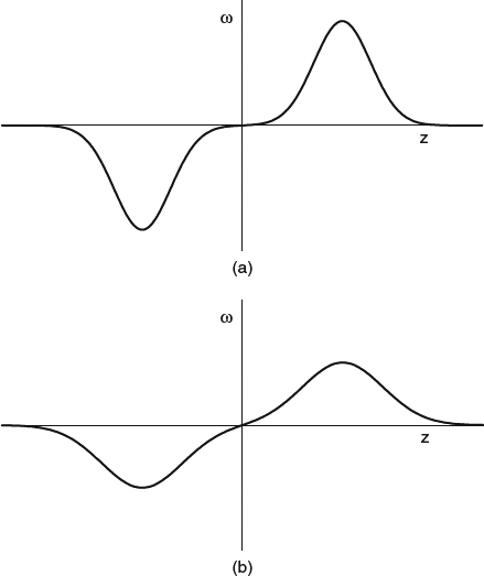
Figure 8.5.7 Diffusion of vorticity in a pair of counter-rotating vortices in 2D unsteady flow. (a) Vorticity in distinct cores at an initial instant. (b) Vorticity diffused into contact with the symmetry plane at a subsequent time

The overall structure this leads to is illustrated schematically in Figure 8.5.8, which shows a plan view of the wake with the streamwise scale greatly compressed so as to fit the entire development on the page. To illustrate the general topology of the vortex lines clearly, we've removed the circumferential component that made the vortex lines appear helical in Figure 8.1.5. In a process that starts with the growth of instability motions and continues through the breakup and postbreakup turbulence, the vortex core on each side of the symmetry plane spreads both inboard and outboard. The vorticity that diffuses toward the symmetry plane turns and reconnects with vorticity on the other side. The wake spreads and becomes more diffuse, and at the same time, the net vorticity (circulation) on each side decreases through the process of reconnection.

So far our argument for reconnection has been indirect: We expect vorticity from both sides to disappear at the symmetry plane, and the only way it can do that is through reconnection. Now let's try to identify a more direct physical mechanism. Reconnection requires the production of a nonzero spanwise component ω_y = −∂w/∂x +∂u/∂z at the symmetry plane. The rotation associated with ω_y must be opposite to that of the bound vorticity on the wing, as illustrated in Figure 8.5.9, and from the sense of the rotation arrows, we can see that this dictates negative ω_y and thus either positive ∂w/∂x or negative ∂u/∂z or both. A positive ∂w/∂x is fairly easy to explain. Looking at the vertical-velocity distribution in the wake oval in Figure 8.1.8a, we can see that when vorticity diffuses out from the center of a vortex core the associated shear-stress gradient has the effect of reducing the circumferential velocities around the core. Thus when vorticity reaches the symmetry plane, it should have the effect of reducing the downwash there. A gradual reduction in the magnitude of the downwash (the negative w) as we move downstream constitutes a positive ∂w/∂x, which is consistent with reconnection. We know that things change slowly in the x direction, so that dw/dx is small, and the corresponding ω_y is weak, which is consistent with a reconnection process that is spread out over a long distance.

Figure 8.5.8 Plan view of the farfield development of the vortex wake of a lifting wing, showing spreading out of vortex cores, vortex-line reconnection, and the formation of closed loops. The streamwise scale is highly compressed to allow showing the entire development in one view

Figure 8.5.9 Illustrating the rotation of the bound vorticity and the reconnecting vorticity at the plane of symmetry far downstream in the vortex wake

As all of this happens, the cross-sectional shape of the wake probably changes in other ways. In addition to the mean vorticity diffusing toward the symmetry plane, some vorticity likely diffuses outward beyond the boundary of the oval and is convected upward relative to the oval, forming a vertical “curtain,” as illustrated in Figure 8.5.10.

This distortion of the vorticity distribution relative to the oval has been observed in 2D unsteady calculations for laminar vortices in a stratified atmosphere (Spalart, 1996), and Figure 8.5.10 is based on the assumption that the same qualitative pattern will occur in the “turbulent” mean flow during instability growth and breakup. The mean velocity distribution in the “curtain” is similar to that in the viscous wake of a 2D body, as in Figure 5.3.1. In the reference frame of the atmosphere, the fluid in a viscous wake flows toward the body that generated the wake, just not as fast as the body is moving away. Similarly, the fluid in the “curtain” is descending relative to the atmosphere, just not as fast as the wake oval from which it came. The velocities in the oval are easier to visualize in the reference frame descending with the oval, and in this frame the vertical velocity in the “curtain” has a conventional-looking wake velocity profile, as illustrated in Figure 8.5.10.

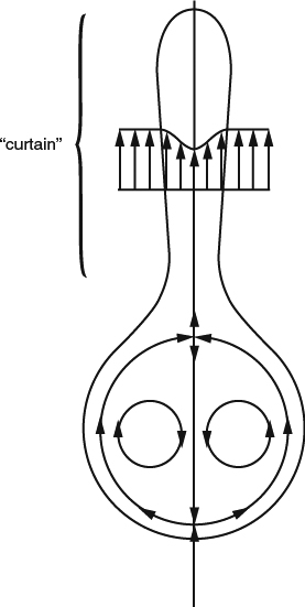
Figure 8.5.10 Change in cross-sectional shape of the vortex wake as vorticity diffuses beyond the boundary of the descending oval. In the reference frame of the descending oval, the distribution of vertical velocity in the “curtain” above the oval is similar to that in a viscous wake

As we move downstream, and the wake becomes more diffuse, the net vorticity on each side decreases, and the descent rate of the oval decreases as well. Thus in side view, the wake should take the general form shown in Figure 8.5.11, in which the oval spreads out, and the “tail” grows taller.

To summarize what we have deduced so far: a time-averaged vortex-wake system as sketched in Figures 8.5.8 and 8.5.11, consisting of closed loops that include the bound vorticity and the trailing vortices, and are closed downstream in a long and diffuse region of time-averaged vortex reconnection. Presumably all of the mean vorticity from the wake upstream eventually disappears through reconnection, though how much of this is complete before the wake encounters the ground is unknown. The ground, being a surface with a no-slip condition and thus capable of generating surface shear stresses, could serve as a sink for some of the vorticity. Of course, much of this is impractical to verify experimentally because the mean-velocity disturbances become much too small to be detected against the background turbulence in the atmosphere. The downstream reconnection of the vorticity is topologically similar to a starting vortex, but it is spread over a very large area, especially in the flight direction. The mean vorticity in the reconnection region is convected freely with the flow, so it is moving downstream at roughly freestream velocity. But at the same time, diffusion of the vorticity by the turbulent motions is such that the entire time-averaged structure moves with the airplane and is steady in the frame of the airplane, unlike the field around an idealized starting vortex.

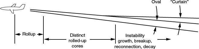
Figure 8.5.11 Side view of the farfield development of the vortex wake of a lifting wing, including the “curtain.” The streamwise scale is highly compressed to allow showing the entire development in one view

The fact that the mean vorticity in the wake disappears in a process that is steady in the reference frame of the airplane raises an interesting question: Does this process produce an integrated pressure disturbance at the ground? In Section 8.5.2, we argued that a starting vortex at high altitude would not do so because the idealized starting vortex was assumed to be steady in the reference frame of the atmosphere, not that of the airplane. Now, in our “real” situation, we have reconnecting mean vorticity (nonzero ω_y) imbedded in a mean flow that is steady relative to the airplane, and we might therefore expect it to produce an integrated pressure disturbance. But this expectation would be incorrect. The spanwise vorticity ω_y in the region of vorticity reconnection is not bound vorticity like that on the wing; it is free vorticity that is convected with the flow. Free vorticity is by definition force-free. Only bound vorticity that experiences a lift force could result in an integrated pressure disturbance. The flow in this region appears steady in the frame of the airplane only because of convection and diffusion, not because the vorticity is bound to a surface carrying a force. As each filament of ω_y is convected downstream, a new one replaces it by convection, and turbulent diffusion maintains the ω_y gradients that allow the whole field to appear steady even though ω_y varies with x.

So much for what happens to the vortex wake. After this process is effectively complete, and the vortex wake has decayed into insignificance, is anything left other than undifferentiated turbulence? Well, if the flowfield hasn't yet interacted significantly with the ground so as to exchange a significant integrated shear force with it, the remaining viscous wake must have a momentum flux deficit corresponding to the total flight-direction aerodynamic force on the airplane, including the induced drag. After all, the assumptions behind Equations 6.1.2–6.1.6 are still satisfied. For an airplane in steady, level, powered flight, the total flight-direction force, including thrust, is zero, and the wake would have no momentum-flux deficit. But for a glider, there would be a deficit (in the flight direction, not the horizontal direction), and after the disappearance of the vortex wake, the wake would have become a viscous wake with a deficit that represents both induced drag and viscous drag.

8.6 Effects of Wing Sweep

Wing sweep can be used to provide better longitudinal stability and trim for a tailless airplane (flying wing), but it is most commonly used to increase Mach-number capability, whether the airplane has a tail or not. Sweep is so effective at increasing critical Mach number that it has become ubiquitous on wings designed to operate at high subsonic speeds. It works because compressibility effects in the wing flowfield are determined more by the component of Mach number perpendicular to the isobars of the flow than by the magnitude of the Mach number. On a swept wing, the isobars tend to sweep more or less with the general sweep of the wing, which can make the perpendicular component of Mach number significantly smaller than the magnitude. This mechanism was first explained by Busemann in 1935 and was classified as a German military secret shortly thereafter. In 1945, it was independently discovered by R.T. Jones at the NACA. See Anderson (1997) for an account of the history of the idea and its incorporation into airplane design. We'll discuss the idealized theoretical argument in Section 8.6.1.

Sweep can also benefit an airplane by providing static aeroelastic relief. Under the high g-loadings that often determine the required strength of the wing structure, a wing generally tends to bend upward. Even if there is no torsional deflection of the structure, a simple bending deflection, when combined with aft sweep, produces an effective geometric twist, leading-edge-down on the outboard wing. The result is reduced loading outboard and reduced bending moments compared with what would happen without the bending. An aft-swept wing can therefore usually have a lighter structure than a comparable unswept wing.

In Section 8.2.1, we discussed the effects of planform on the spanload of a 3D wing, and in Figure 8.2.2, we saw how aft sweep moves the additional load due to angle of attack outboard. Because of this effect, aft-swept wings must generally be twisted leading-edge down, or washed out, to have an advantageous total spanload like that shown in Figure 8.2.2. A favorable spanload that is achieved in this way persists only over a limited range of angle of attack.