3

Continuum Fluid Mechanics and the Navier-Stokes Equations

The Navier-Stokes (NS) equations provide us with a nearly all-encompassing, highly accurate physical theory that can predict practically all phenomena of interest in aerodynamics, including “aerodynamic” flows of liquids such as water. In Section 3.1, we briefly consider the general way in which these equations represent the physics, the assumptions that had to be made to arrive at them, and their range of validity. Then in the sections after that, we delve into the specifics of the equations and what they mean.

3.1 The Continuum Formulation and Its Range of Validity

In the NS formulation, the fluid is treated as a continuous material, or continuum, with local physical properties that can be represented by continuous functions of space and time. These continuum properties, of course, depend on the properties of the molecules that make up the gas or liquid and on the lower level physics of their motions and interactions. However, the continuum properties represent only the integrated effects of the lower level physics, not the details. As I noted in Chapter 2, this provides a representation that is not merely adequate, but highly accurate over a wide range of conditions.

The early historic development of the NS formulation followed an ad hoc approach, assuming continuum behavior a priori and developing a model for the effects of viscosity based on experiments in very simple flows. Much of the hard work involved in this development was devoted to the development of the mathematical formalism that was required to generalize from simple flows to more general ones. We'll touch again on mathematical formalism issues in Section 3.2.

The NS formulation can also be derived formally from the lower level physics, with simplifying assumptions to get rid of the dependence on the details. For gases, the appropriate next lower level to start from is a statistical description of the motion of the molecules and the conservation laws that apply to them, as embodied in the Boltzmann equations. With reference to this kind of derivation, the statement that continuum properties represent only “integrated effects” takes on a literal meaning. We use time-and-space averaging, that is, integration, over molecular motions to define the continuum properties of the flow at every point in space and time: the density and temperature of the fluid, and its average velocity. For the definitions of these basic flow quantities, we don't have to make any simplifying assumptions beyond the averaging process itself and that the fluid must be sufficiently “dense” for the averages to “converge.” This “convergence” problem is one we'll consider in more detail below.

Although the averaging process gives us rigorous definitions of our basic continuum flow quantities, it doesn't get us all the way to the NS formulation. When we apply the averaging process to the basic conservation laws for mass, momentum, and energy, we get two different types of terms that represent separate sets of phenomena and end up requiring different assumptions:

1. Terms in which only the simple averages defining the continuum density, temperature, and velocity appear explicitly. No further assumptions are needed because these are already the basic variables of the NS formulation. Terms of this type represent the local time rate of change of a conserved quantity or the convection of a conserved quantity by the local continuum velocity of the flow.
2. Terms that involve averages of products of molecular velocities or products of a velocity component and the kinetic energy. Such terms represent transport of a conserved quantity relative to the local continuum motion of the flow. The transport of thermal energy is just the heat flux due to molecular conduction. The transport of momentum has the same effect as if a continuum material were under an internal stress and is thus the source of both the local continuum hydrostatic pressure and the additional continuum “stresses” due to viscous effects. The averaging process alone leaves these terms in a form that still depends on statistical details of the molecular motions, and further simplifying assumptions are required to get them into forms that can be expressed as functions of our basic continuum flow variables.

In the NS equations, the terms representing the above transport phenomena have very simple functional dependences on local continuum properties. The hydrostatic pressure is given by an equilibrium thermodynamic relation (an equation of state). The heat flux and the viscous “stresses” are given by gradient-diffusion expressions in which the flux of a conserved quantity is proportional to a gradient of the conserved quantity. Fluids exhibiting the simple behavior of the viscous stresses described in the NS equations are often referred to as Newtonian. To get to these simple forms from the general ones that we get from the averaging process requires some simplifying assumptions about the physics. For gases, we must assume the fluid is everywhere locally near thermodynamic equilibrium. This means that the probability distribution functions for molecular velocity that appear in the full transport expressions must be near their equilibrium forms, which in turn requires that significant changes can take place only over length and time scales that are long compared with the mean-free path and time. When these conditions are satisfied, that is, when the local deviations from equilibrium are small, the transport-related terms can be represented very accurately by the simple relationships we use in the NS equations.

The main relationships comprising the NS equations are the basic conservation laws for mass, momentum, and energy. To have a complete equation set we also need an equation of state relating temperature, pressure, and density, and formulas defining the other required gas properties. For aerodynamics applications it is usually a good approximation to assume the ideal gas law, along with a constant ratio of specific heats (γ) and viscosity and thermal conductivity coefficients (μ and k) that depend on temperature only. It seems counterintuitive that the transport coefficients μ and k are well represented as being independent of density at constant temperature, but there is a simple way to understand why this is. As density increases, one might think that the transport coefficients should increase as well because there is more mass per unit volume to transport momentum and thermal energy. However, as density increases, the molecular mean free path decreases, which hinders molecular transport. At the ideal-gas level of approximation, the effects of increasing mass per unit volume and decreasing mean free path exactly offset each other. Thus, practically speaking, the effectiveness of molecular transport depends only on the average speed of the molecules, or the temperature. In some forms of the equations, the local speed of sound (“a”) appears, which for an ideal gas also depends only on temperature.

The NS equations, like any field equations, need boundary conditions (BCs). At flow boundaries, where the flow simply enters or leaves the domain, the NS equations themselves determine what combinations of BCs can be imposed and what combinations are required to “determine” the solution in various ways. For boundaries that are interfaces with other materials, for example, gas-solid or gas-liquid interfaces, the NS equations themselves don't fully define the situation, and we need to introduce additional physics. According to theoretical models and experimental evidence, the interaction between most of the liquid and solid surfaces encountered in engineering practice and air at most ordinary conditions is such that the continuum velocity and temperature of the air accommodate almost perfectly to the velocity and temperature of the surface. Thus assuming no slip and no temperature jump at the “wall,” and imposing BCs accordingly, is an extremely good approximation.

A correct physical interpretation of the no-slip BC requires care. In some popular descriptions, the fluid is said to “stick” or “adhere” to the surface. This description is not completely inappropriate, but it is misleading, especially in the case of gasses. Saying that something “adheres” conjures up an image of a bond that can withstand tension as well as shear. Of course a gas cannot be put in tension at all, let alone form a tension-resisting bond with anything else. But the no-slip condition does assume no sliding between the fluid and the solid, so that with regard to shear, the fluid does behave as if it were adhering to the surface.

The no-slip condition applies to both liquids and gasses. How it comes about is easier to explain in the case of a gas. While an occasional gas molecule may adhere temporarily to a solid surface (or react chemically with it and remain more permanently), an overwhelming fraction of the molecules that impinge on the surface bounce off. The no-slip condition arises from the nature of these bounces. First, imagine the gas molecules as smooth spheres bouncing specularly off a smooth surface and not losing any tangential momentum in the process. In this case, there would be no shear force exchanged between the surface and the gas, the gas would slip easily along the surface, and there would be no no-slip condition. But on the scale of the molecules, no real surface acts as a smooth surface. All real surfaces consist of atoms similar in size to the gas molecules, and thus even the smoothest is rough on the scale of a gas molecule. And most real surfaces have considerable roughness on larger scales as well. The upshot is that gas molecules impinging on real surfaces bounce off in effectively random directions, which forces the average tangential velocity of molecules near the surface to be very small. Kinetic theory can be used to estimate the effective slip velocity (see White, 1991, Section 1-4.2), showing that in practical situations it is practically zero. And this must be true even for surfaces that feel slick to the touch, for which our intuition wrongly imagines air being able to slide freely.

Thus our complete physical model consists of the NS equations combined with the no-slip and no-temperature-jump BCs. The range of applicability of this formulation is very broad, and there are only a few applications of practical “aerodynamics” interest where it doesn't apply. Some examples of such exceptions are gas flows at very low densities (for example, very high altitude) and the detailed internal structure of shock waves. Even flows in which ionization, dissociation, or chemical reactions take place are not generally exceptions, because such effects can be incorporated into our continuum formulation by the inclusion of appropriate species-concentration variables, reaction-rate equations, and equations of state. Fortunately for us in aerodynamics, we don't have to deal with the complexities of non-Newtonian liquids, which are important in biological systems and many industrial processes.

So what is it that causes our NS formulation not to apply in the exceptional situations? Is it that very low densities in very high altitude flight, or very small length scales as in the shock-wave problem, cause our averaging process not to converge, a possibility I alluded to earlier? This can happen, but in many cases it is not the cause of “failure.” Of course, at a single instant in time, the convergence of a spatial average would require integrating over a large enough volume to include a large number of molecules. Such instantaneous spatial averages might not resolve the internal structure of a shock wave very well, for example, but many flows are close enough to being steady that we can get around this problem and define averages in small spatial volumes by averaging over a sufficiently long period of time. I would think that most of the interesting cases of flight at extreme altitudes or of detailed shock-wave physics can be resolved in this way. In these cases, then, the “failure” of our continuum formulation comes not from the failure of our averaging process to converge, but from the failure of the local-thermodynamic-equilibrium assumption behind our modeling of the “transport” effects when flow gradients become significant on the scale of a mean-free path. Another thing that tends to happen under such conditions is that the errors inherent in the no-slip and no-temperature-jump BC, negligibly small under “ordinary” conditions, become much bigger fractions of the differences in flow quantities in the rest of the field, and these approximations break down as well.

3.2 Mathematical Formalism

Now let's consider some of the issues that arise in casting our formulation of the physics in mathematical terms. Our final formulation will take the form of a set of partial-differential field equations (PDEs), along with some algebraic auxiliary relations. The variables we use, as well as which variables are independent and which are dependent, depend on how we choose to describe the flow. We can choose to describe it in terms of what happens as seen at “fixed” points in space and time, the so-called Eulerian description, or we can choose to define the trajectories of “fixed” parcels of fluid as they evolve in time, the Lagrangian formulation. In the Eulerian description, time and the coordinates in some spatial reference frame, which may or may not be inertial, are the independent variables, and the velocity, pressure, and other state variables of the fluid are dependent. In the Lagrangian description, the independent variables identify the fluid parcels, for example, in terms of their spatial coordinates at an initial instant, and the dependent variables include the spatial coordinates of the parcels at succeeding instants. These two modes of description are in principle equivalent in the sense that they can be used to model exactly the same physics, but they do it in such different ways that they are not practically interchangeable.

For most purposes, the Eulerian framework is more convenient and is therefore the basis for nearly all quantitative work in theoretical aerodynamics and computational fluid dynamics (CFD). A major reason for this is that the Eulerian description provides a much more natural framework for treating steady flows, which are the predominant focus of aerodynamics. All of the higher level conceptual modeling we'll encounter involves the Eulerian description, but we'll still find it helpful to invoke the Lagrangian description in some of our discussion of the basic physical laws.

The time rate of change of any physical quantity (e.g., velocity and temperature) associated with a Lagrangian fluid parcel is called the Lagrangian derivative and is usually denoted by the upper case D/Dt. This Lagrangian rate of change is made up of contributions from either or both of two effects, as seen in the Eulerian frame. First, the quantity may be changing with time at the points in space through which the parcel is moving, as reflected in the unsteady-flow term ∂/∂t, or the Eulerian rate of change. Second, if the parcel is moving with velocity V through a nonuniform field, it must experience a rate of change in addition to the unsteady-flow term. In general, then, the Lagrangian derivative is related to derivatives in the Eulerian frame by

This transformation has interesting consequences when we apply it to the fluid velocity, to determine the Lagrangian acceleration. For example, for the simplest case of a 1D steady flow, Equation 3.2.1 applied to the velocity reduces to

From this we see that a given material acceleration Du/Dt requires a large spatial gradient ∂u/∂x when u is small, but only a small ∂u/∂x when u is large. This is a consequence of a Lagrangian fluid parcel's motion through the velocity field. In Section 3.4.6, we'll look at how the convective acceleration appears in the convective terms in the momentum equation, and in Sections 4.1.2 and 4.2.1 we'll consider it again in the context of boundary-layer flows.

A factor that complicates the mathematics is that some of the quantities we must deal with are vectors and tensors. The velocity is a vector, and the equation for conservation of momentum is a vector equation. In 3D, this results in three variables and three of our equations, which is a pretty straightforward thing to grasp intuitively.

What is less intuitive is the problem of representing the transmission of forces by “contact” between adjacent fluid parcels. Physically speaking, of course, these forces are a result of momentum transfer by molecular motions, but in the continuum formulation the integrated effects of the motions of many molecules are represented as apparent internal stresses in the fluid, or forces per unit area of the boundary of a parcel. We'll encounter this idea again in our discussion of the momentum equation in Section 3.4.2. The mathematical problem we face is the general problem of representing the state of stress in a continuous material. First, we have to get used to the idea of imaginary boundaries separating adjacent parcels of material. Then we must visualize how any two adjacent parcels exert equal-and-opposite stresses on each other across their common bounding surface. Our description must be able to define the state of stress at any point in the fluid in such a way that it gets the right value for the opposing forces for any orientation of the imaginary boundary. The stress is a force per unit area (a vector) that depends on the orientation of an imaginary dividing surface, which can be defined by the direction of the normal to the surface (another vector).

The stress is thus a tensor. An entire field of mathematics, tensor analysis, was developed just to provide rigorous means for mathematical manipulation of such quantities, not just in continuum mechanics, but in other branches of physics as well, and along with it came powerful shorthand notations for expressing the manipulations. Tensor notation provides the least error-prone way to deal with the stress terms and convection terms in our equations, especially when it comes to deriving the many terms that arise when the equations are transformed to different coordinate systems. Such manipulations can be done without tensor notation, but avoiding errors becomes much more difficult. With or without tensor notation, however, such manipulations quickly become exercises in manipulating symbols, and it can be difficult to maintain any grasp of the physical meaning. We'll try to reach a physical understanding of the most important aspects of the viscous stresses by using very simple flow situations as examples in Section 3.6.

So far, we have talked about the NS equations only in their local or differential form, which is the form that will relate most directly to most of our succeeding discussions. However, in some applications, a more global view of the flow suffices and can be easier to deal with. For these situations, we have the control-volume form of the equations, in which the equations have been integrated over a volume and the surfaces bounding the volume. The control-volume equations are “exact” in the sense that there is no loss of accuracy relative to the differential equations, but they are “simplified” in the sense that they can tell us only what happens to integrated quantities and nothing about how the local quantities are distributed over the volume and bounding surfaces. We'll use the control-volume approach to calculate viscous drag in Section 6.1.4 and lift-induced drag in Section 8.3.2, and we'll consider the general approach further in Chapter 9.

In ordinary solutions to the NS equations, all flow quantities are continuous and differentiate, even through shocks (see more about shocks in Section 3.11.2). This brings some powerful mathematical facts to our aid, without our having to introduce any “physics” at all, which brings us to the topic of the next section.

3.3 Kinematics: Streamlines, Streaklines, Timelines, and Vorticity

Kinematic descriptions are basic to all our attempts to understand flowfields. Obviously, we must understand the kinematic structure of a flow before we can understand the underlying dynamics. The kinematic structure of a flowfield is constrained to have certain characteristics because the velocity field is a continuous vector field.

3.3.1 Streamlines and Streaklines

Two kinematic concepts we often appeal to are streamlines and streaklines. Streamlines are simply 3D space curves, defined as being everywhere parallel to the velocity vector. A streakline is also a 3D space curve, but is defined by the locations of a string of Lagrangian fluid parcels that all passed through a given “point of origin” somewhere upstream in the flowfield. (We introduced the Lagrangian description of the flowfield in Section 3.2, and we'll define what a Lagrangian fluid parcel means more precisely in Section 3.4.) The point of origin for a streakline is usually taken to be a fixed point in space, but it needn't be; it can be allowed to move with time. A streamline is obviously a mathematical construct that can be defined only by “solving” a mathematical problem, that is, “construct a curve everywhere parallel to a given vector field.” A streakline, on the other hand, can be “realized,” at least approximately, in real flows that are marked by a passive contaminant such as dye in liquids or smoke in air.

If the flow is steady, streamlines and streaklines from fixed points of origin will coincide and will be the same as individual particle paths, that is, the paths of individual Lagrangian parcels. Even in steady flows, however, interesting issues can arise in the interpretation of flow patterns. Figure 3.3.1, for example, compares a streamline pattern constructed from a steady-flow CFD solution with the corresponding nominally steady streakline pattern marked by dye in a water tunnel. The two patterns should of course be the same, and on close inspection they agree about as well as a CFD calculation and an experiment can be expected to. But at a glance, the two images give very different impressions. In the CFD solution, the separation at about 60% chord and the formation of a closed separation bubble stand out clearly, while in the water-tunnel photo the separation is evident only if you look very carefully. Part of the problem is that the field of view of the photo doesn't show the whole length of the separation bubble. I must admit that I didn't realize that this flow separates ahead of the trailing edge until I saw the CFD streamlines. And I'm in good company: Van Dyke (1982) published this same photo with the comment that the flow “appears to be unseparated.”

If the flow is unsteady, the situation is much more complicated, and streamlines, streak-lines, and particle paths will generally all be different. Looking at the pattern formed by any one of them gives an incomplete and usually misleading picture of the flow. Figure 3.3.2 shows how different the unsteady flow in the wake of a circular cylinder looks in terms of streaklines (a) and streamlines (b). Timelines (c), which we'll define in Section 3.3.3, also present a very different picture.

3.3.2 Streamtubes, Stream Surfaces, and the Stream Function

The concept of a streamtube is one that is usually applied only to steady flows. The definition of a streamtube starts with a closed curve in the flowfield, as illustrated in Figure 3.3.3a. Steady streamlines or streaklines passing through all points on the curve define a surface that forms the boundary of a curvilinear tube. Because the bounding surface is parallel to the velocity vector, no continuum fluid parcel passes through it. In a steady flow, according to the principle of continuity, which we'll discuss in the next section, the mass flux in a streamtube is the same at any cross section along its length. In a 2D flowfield, we could still define a streamtube the same way we did in 3D, using a closed curve to define the boundary, but a more useful definition is to allow the closed curve defining the streamtube to degenerate into two points, so that the streamtube becomes a 2D layer of flow defined by one streamline through each point, as illustrated in Figure 3.3.3b.

The bounding surface of a streamtube is a special case of the more general concept of a stream surface, which also is usually applied only to steady flows. The space curve from which a stream surface originates needn't be a closed curve, and a stream surface needn't form a closed tube. A general stream surface is also a surface through which no continuum fluid parcel passes. In 3D flows, stream surfaces that start out relatively flat can become highly contorted as the flow progresses downstream.

Figure 3.3.1 Streamlines and streaklines in the entirely laminar steady flow around a NACA 64A015 airfoil at zero incidence, R = 7,000. (a) Streamlines in a steady-flow CFD solution showing a separation bubble starting at about 60% chord. Laminar RANS calculation by Steven R. Allmaras. (b) Streaklines marked by dye released from upstream in a water tunnel. The streaklines closest to the trailing edge apparently consist of dye streaming forward from the closure region of the separation bubble, beyond the right edge of the photo. Aft of mid-chord there are variations in streakline spacing that are not present in the CFD solution. Photo by Werle, 1974, courtesy of ONERA

Figure 3.3.2 Unsteady wake (von Karman vortex street) of a circular cylinder at Reynolds numbers in the range 136–140. Photos by S. Taneda, © SCIPRESS. Used with permission. (a) Streaklines marked by dye introduced at the cylinder surface. (b) Streamlines approximated by short time exposure of suspended particles. Used with permission. Photos by S. Taneda, © SCIPRESS. Used with permission. (c) Timelines marked by hydrogen bubbles from a pulsed wire upstream. Photos by S. Taneda, © SCIPRESS. Used with permission

Figure 3.3.3 Illustrations of streamtubes. (a) As a compact streamtube defined by a closed contour in a 3D flow. (b) As a sheet of flow defined by two points in a 2D flow

The stream function is a concept that applies only to 2D flows. Considering any two points A and B in a 2D flow, the mass flux across any curve joining the two points depends only on the locations of the points and on time, provided the flow is either incompressible or steady. (For example, for the two points in Figure 3.3.3b, the mass flux across any contour joining the points is the mass flux in the shaded streamtube.) Thus if we fix point A, the mass flux defined in this way for all other points B defines a single-valued function we call a stream function. It follows then that the stream function is constant along streamlines and that the difference in its value between two streamlines is the mass flux in the streamtube bounded by them. The stream function was used more frequently in the past than it is now. It was often used in earlier theoretical discussions of incompressible flows (see Section 3.10) and was sometimes used in numerical methods for solving the NS equations in 2D.

3.3.3 Timelines

Another useful kinematic concept is that of timelines, which are usually considered most useful in 2D flows, though they can be defined in any flow, steady, or unsteady. The definition starts with the marking of a string of Lagrangian fluid parcels arrayed across the flow at some initial instant. A timeline is then the space curve defined by that same string of parcels at some future instant. Timelines are most useful when defined in sets of multiple lines whose initial instants are separated by equal time intervals. In real flows, timelines can be realized approximately by passive-contaminant markers, usually emanating from a fine wire stretched across the flow. In air, the wire is coated with oil, and a pulsed electric current in the wire produces brief puffs of smoke, marking cross-stream lines that convect downstream. In water, electric pulses can produce lines of tiny hydrogen or oxygen bubbles that mark the flow. In Figure 3.3.2c, we saw timelines in the flow past a circular cylinder.

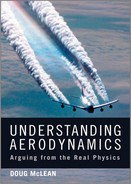
Figure 3.3.4 shows an example of timelines in a turbulent boundary layer, illustrating a key aspect of timelines in turbulent flows. In a fully turbulent boundary layer, the turbulent velocity fluctuations are not large fractions of the mean velocity, and as a result, the younger timelines near the left edge of the photo remain ordered and build up distortions slowly, looking as if they were in a smoother flow than that in the rest of the photo. As the flow progresses from left to right, the distortions accumulate until, in the right half of the photo, the timelines that are entirely inside the boundary layer appear as a chaotic jumble. In this fully turbulent flow, the timeline picture gives the misleading impression that the intensity of the turbulent motions is increasing from left to right. In steady flows, timeline patterns tend to be simpler and less prone to misinterpretation, as we'll see later in the case of a circular cylinder in ideal potential flow in Figure 5.1.3c.

3.3.4 The Divergence of the Velocity and Green's Theorem

The fact that the velocity is a continuous and differentiable vector field also means that the usual theorems of vector analysis apply. Some constrain the physics in ways that can simplify our task considerably.

Green's theorem relates the divergence of the velocity to a surface integral:

where the triple integral is over any volume occupied by the fluid, and the double integral is over the surface that encloses the volume. This is a key ingredient in derivations of the control-volume forms of the equations.

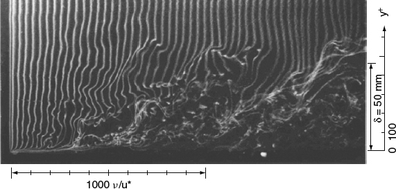
Figure 3.3.4 Timelines in a turbulent boundary layer in water, marked by hydrogen bubbles from a pulsed wire at the left edge of the photo. From Y. Iritani, N. Kasagi and M. Hirata © (1980). Used with permission

3.3.5 Vorticity and Circulation

Relationships involving the vorticity are extremely useful for purposes both of conceptualizing and doing quantitative calculations. In this section, we'll concentrate on the kinematics of vorticity and its relationship to the velocity field. We'll encounter the Biot-Savart law, which leads naturally to the idea of vortex induction, and we'll take pains to come to a correct understanding that induction is not a dynamic phenomenon, as implied by the way people often talk about it, but is instead a strictly kinematic concept. The real dynamical aspects of vorticity are yet to come, in Sections 3.6 and 3.8 and in the discussion of lift in Chapters 7 and 8.

The vorticity is just the curl of the velocity:

from which it follows by a basic vector-calculus identity that the vorticity is divergence free:

If we know the vorticity at a point in a flowfield, we know something about how the velocity varies in the neighborhood of that point, but we don't know everything. In a constant-density flow, the deviations in velocity in the neighborhood of a point can be expressed as the sum of two parts: a deformation velocity field and a solid-body rotation with angular velocity ω/2, a result known as Helmholtz's first theorem (see Milne-Thomson, 1966, Section 3.22). Examples of how these two components of motion look in isolation and in combination in 2D flow are illustrated in Figure 3.3.5. In each sketch, a square fluid parcel and perpendicular lines bisecting it at an initial instant are shown as solid lines, and the same lines anchored in the fluid are indicated at a later instant by dashed lines. Because we're interested in velocity deviations, we anchor our reference frame to the fluid at the center of the square and show the center as not moving. In Figure 3.3.5a we have a pure solid-body rotation in which the two bisecting lines have rotated in the same direction by the same amount. In Figure 3.3.5b we have a pure deformation in which the vorticity, and therefore the average angular velocity of the fluid, are zero. This is reflected in the fact that the bisecting lines have rotated by equal-and-opposite amounts. In Figure 3.3.5c we have added components Figure 3.3.5a,b together. The result is a simple shearing motion in which the horizontal bisecting line hasn't rotated at all, and the vertical bisecting line has rotated twice as far as in either Figure 3.3.5a or b. The average angular velocity, and thus the vorticity, are the same as in Figure 3.3.5a. These examples are 2D, but they are indicative of what these effects would look like in 3D in planes perpendicular to the vorticity vector.

Figure 3.3.5 Illustrations of the effects of solid-body rotation and deformation on initially square fluid parcels in 2D flow. The square and perpendicular lines bisecting it at an initial instant are shown as solid lines, and the same lines anchored in the fluid are indicated at a later instant by dashed lines. (a) A pure solid-body rotation in which the two bisecting lines have rotated in the same direction by the same amount. (b) A pure irrotational deformation in which the vorticity, and therefore the average angular velocity of the fluid, are zero. This is reflected in the fact that the bisecting lines have rotated by equal-and-opposite amounts. (c) Components (a) and (b) added together. The result is a simple shearing motion in which the horizontal bisecting line hasn't rotated at all, and the vertical bisecting line has rotated twice as far as in either (a) or (b). The average angular velocity, and thus the vorticity, are the same as in (a)

The deviation velocity components comprising the solid-body rotation part of the motion are in a plane perpendicular to the vorticity vector, but there is no such constraint on the deformation part. Note that the vorticity does not determine the deformation part of the field, but that the vorticity and the solid-body-rotation part of the field are proportionally related. Thus at any point where the local velocity field has a solid-body-rotation component to it, the vorticity must be nonzero. Likewise, if the vorticity is zero, there is no solid-body rotation component, and because of this, flows with zero vorticity are often called irrotational.

Much of our theorizing in subsequent sections will make use of the interplay between vorticity and the circulation, which is defined as the line integral of the velocity around a closed contour. The crucial relationship is given by Stokes's theorem:

where the double integral is over any continuous surface that is bounded by the contour and is piecewise smooth over its entire area, as shown in Figure 3.3.6. For Equation 3.3.4 to hold, the integrands need merely to be integrable; they needn't be continuous. Thus creases in the surface are allowed, because they occupy zero area, or a subset of zero measure, as the mathematicians would say. Likewise, kinks in the closed contour are allowed.

What Stokes's theorem says, in words, is that the circulation around a closed contour is equal to the flux of vorticity through the contour. When we discuss dynamics in Section 3.8, we'll find this relation useful for drawing conclusions about the persistence of the circulation, or lack of circulation, and often we'll be able to do so without any actual calculation.

Figure 3.3.6 Illustration of a closed contour and bounded surface to which Stokes's theorem applies

3.3.6 The Velocity Potential in Irrotational Flow

If the flow is irrotational (zero vorticity everywhere), we can derive a further useful result from Equation 3.3.4, which now states that the circulation around any closed contour must be zero. We start by noting that for any two points A and B in the field, we can define many different closed paths from A to B and back to A. Because the line integral of the velocity around any of these paths must be zero, the line integral along one path segment from A to B must be the negative of the line integral along the other path segment from B to A, and because this must be true for any choice of the two path segments, both line integrals must be independent of the path taken. Now if we fix point A, the line integral from A to any other point B is a single-valued scalar function of the location of point B, and it is easy to show that the velocity vector must be equal to the gradient of that function. Thus whenever the velocity field is irrotational, it can be expressed as the gradient of a scalar function we call a velocity potential ϕ:

The existence of a velocity potential can greatly simplify the analysis of inviscid flows by way of potential-flow theory, which we'll discuss further in Section 3.10. In the above discussion, we assumed the simplest situation, in which the vorticity is zero everywhere. However, many of the situations in which potential-flow theory is applied are not so simple. Many practical flows are effectively irrotational everywhere except for isolated concentrations of vorticity. Potential-flow theory can still be applied in the irrotational parts of these flows, but special treatments are required to account for the presence of the isolated vorticity. Examples include the jumps in velocity potential that must be allowed across vortex sheets, as discussed in Section 3.3.7, and the special treatment required in the potential-flow theory for 2D airfoils, for which the region of irrotational flow is not simply connected, as we'll discuss further in Section 7.1.

3.3.7 Concepts that Arise in Describing the Vorticity Field

We have a variety of concepts that are useful for thinking about how vorticity is distributed in the flowfield. The first ones we'll consider are applicable to the usual realistic situation in which vorticity is continuously distributed.

Anywhere that the vorticity is nonzero, we can define a vortex line as a curve in space that is parallel to the vorticity vector, just as a streamline is parallel to the velocity vector. So a vortex line in the vorticity field is analogous to a streamline in the velocity field, and just as we extended the concept of a streamline to define a streamtube, we can extend the concept of a vortex line to define a vortex tube. By definition, the flux of vorticity across the bounding surface of a vortex tube is zero. This, combined with Equation 3.3.3, means that the flux across any cross-section of the tube, anywhere along its length, is the same.

The fact that the vorticity flux in a vortex tube is constant dictates the changes in vorticity magnitude that must accompany vortex stretching. If the cross-sectional area of a vortex tube decreases, either in time or along the length of the tube, the strength of the vorticity (the magnitude of the vorticity vector) must increase. For a section of vortex tube containing a given amount of fluid, a reduction in cross-sectional area usually requires an increase in length, or a stretching. (It definitely requires it if the fluid density is constant, for reasons we'll discuss in Section 3.4.1 in connection with the conservation of mass.) Thus the stretching of a vortex tube usually increases the local vorticity magnitude.

A vortex filament is a vortex tube whose cross section has a maximum dimension that is infinitesimally small. The cross-sectional area of a vortex filament is thus also infinitesimally small, but it is still assumed to vary along the length of the filament, so that the filament can still satisfy the definition of a vortex tube. For a vortex filament, the flux of vorticity across a cross-section reduces to the product of the vorticity magnitude and the cross-sectional area, which is called the intensity of the filament. Note that this definition of the intensity as the flux of vorticity through an infinitesimal area is different from other concepts of intensity you may be familiar with, for example, the intensity of a light beam, which is defined as the energy flux per unit area. The result that the intensity of a vortex filament is constant along its length is Helmholtz's second theorem (see Milne-Thomson, 1966, Section 9.31). This conservation of intensity means that a vortex filament cannot end anywhere inside the fluid domain and must either form a closed loop (vortex loop) or end on the boundary of the domain.

Depending on the nature of the boundary, there will be constraints on how vortex filaments or vortex lines can end there. First, consider the special case of an isolated vortex filament that is surrounded by irrotational flow. If the flow is steady, and the boundary is an interface across which the fluid cannot flow, such a vortex filament can intersect the boundary only in the normal direction. This is so because there must be an essentially circular flow pattern in the neighborhood of the filament, in planes perpendicular to the filament, as we'll see in Section 3.3.8. This would violate the no-through-flow condition at the boundary if the filament were not normal to the boundary. Further, if the boundary is a stationary solid surface at which the no-slip condition applies, the velocity components in planes perpendicular to the filament must vanish at the wall, and the vorticity magnitude must go to zero. Thus an isolated vortex filament cannot end at all at a solid surface with a no-slip condition.

In the more general case of distributed vorticity, vortex lines may intersect a no-through-flow boundary at which there is slip, and the intersection need not be in the normal direction. On the usual kind of stationary surface with no slip, the situation is much more constrained. Because the tangential velocity is zero on the surface, the component of vorticity normal to the surface must be zero everywhere on the surface. Then if the magnitude of the vorticity is nonzero, the vortex lines must be tangent to the surface. In the viscous flow about a stationary body, this applies practically everywhere on the surface. The only exceptions are isolated singular points of separation or attachment, which we'll discuss further in Section 5.2.2 and which are places where the magnitude of the vorticity on the surface is zero. At such a point, a vortex line may intersect the surface in the normal direction, but it does so with a “whimper,” because the normal component of the vorticity must still go to zero where the line intersects. Thus vortex lines can intersect a no-slip surface only at isolated singular points. It is sometimes erroneously stated that vortex lines cannot intersect a no-slip surface at all, without acknowledgment of the above exception (as pointed out by Saffman, 1992; Section 1.4).

So we see that when vortices approach a solid no-slip surface anywhere other than at an isolated singular point, the vortex lines must turn to avoid intersecting the surface, and in doing so they often become part of the vorticity in a viscous boundary layer on the surface. Figure 3.3.7 illustrates one such situation, the “inlet vortex” that often forms when an engine inlet is near the ground, in this case made visible by water droplets. Lines were added to the photo to illustrate how the vortex lines must spread out in all directions along the ground in this situation. (There is often a spiral component to the vortex lines' alignment, which is omitted here for clarity.) Though this vortex is not a single thin filament, it is fairly concentrated and is surrounded by mostly irrotational flow. Just outside the boundary layer on the ground, the vortex is close to perpendicular to the ground, roughly in keeping with our conclusion above that an isolated vortex filament must approach a no-throughflow boundary in the normal direction.

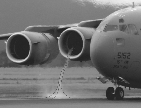
Figure 3.3.7 An inlet vortex marked by water droplets. Because all but one of the vortex lines cannot end on a solid surface with a no-slip condition, the vortex lines must spread out in the boundary layer on the ground as illustrated. The possible spiral component to the vortex lines' alignment is omitted here for clarity. Modified from original photo by Alastair Bor. Used with permission

Now let's consider concepts that were developed for idealized models of flows with highly concentrated vorticity. Concentrations of vorticity in limited regions are important features in some flows we'll study later. For example, as we'll see in Chapter 8, the vorticity in the wake behind a lifting wing starts out concentrated in a relatively thin shear layer and ends up concentrated in two isolated, more or less axisymmetric vortices, all surrounded by practically irrotational flow. In conceptual models of such flows, these vortical structures are often idealized as mathematically thin concentrations, with the shear layers idealized as vortex sheets, and the vortices as line vortices. These idealized entities carry vorticity fluxes that are finite even though the vorticity is concentrated in a region with zero cross-sectional area. The vorticity distribution must therefore be singular, or infinite, at the location of the sheet or line. For a vortex sheet, we must generally integrate over a cut through a finite width of sheet to find a finite flux of vorticity, though the area we have integrated over is still zero, because the sheet is infinitely thin. For a line vortex, we need only integrate over a single cut through the line (a point) to find a finite flux. There is a formal mathematical theory that makes all of this rigorous, but we won't go into it here because the concepts can be understood well enough without it.

A line vortex looks superficially similar to the vortex filament we defined earlier, but there are crucial differences. The cross-sectional area of a line vortex is zero, while that of a filament is infinitesimal, and the vorticity flux of a line vortex is finite, while that of a filament is infinitesimal. We must also take care not to confuse a line vortex, which is a singular distribution of vorticity, with a vortex line, which is simply parallel with the vorticity vector, usually in fields in which vorticity is continuously distributed.

A line vortex in a 2D planar flow is often called a point vortex, because it must be a straight line that extends to infinity in both directions perpendicular to the 2D plane and therefore appears as a single point in the 2D plane. The line vortex is one of the elementary singularities that can be used as a building block to construct solutions in potential-flow theory, as we'll discuss further in Section 3.10. In more general flows, a line vortex would usually be curved, a situation that raises a special problem. At any point on a line vortex where the curvature of the vortex is nonzero, the fluid velocity at that point on the vortex, in a direction perpendicular to the vortex, must be infinite. This makes it impossible to determine a realistic velocity at which such a vortex line will be convected by the flow. (Convection of vorticity is discussed in Sections 3.6 and 3.8.) In real flows, the vorticity is spread out continuously and has finite magnitude, and such infinite velocities do not occur.

3.3.8 Velocity Fields Associated with Concentrations of Vorticity

We've just seen that highly concentrated vorticity is often idealized as a vortex sheet or a line vortex. With Stokes's theorem in hand, we are in a position to determine the nearfield velocity distributions that must accompany these idealized distributions of vorticity, as illustrated in Figure 3.3.8.

A vortex sheet in 2D flow is shown in Figure 3.3.8a. By applying Stokes's theorem to a small closed contour inclosing a short section of the sheet, we see that there must be a jump in velocity magnitude across the sheet equal to the local vorticity strength, or vorticity per unit distance along the sheet in the direction perpendicular to the vorticity vector. In this 2D case, the vorticity vector is perpendicular to the plane of the paper, and the distance along the sheet is measured in the flow direction. The physical flow corresponding to this idealized vortex sheet is a shear layer with the velocity jump spread across a finite thickness, as shown in Figure 3.3.8b.

In a 3D flow, the velocity jump across a vortex sheet, in a vector sense, must still be perpendicular to the vorticity vector. A common situation in aerodynamics, as we'll see in the modeling of wing flows in 3D in Chapter 8, is to have a sheet with no jump in velocity magnitude, only in direction. In this case, the jump in the velocity vector is perpendicular to the vorticity vector, which is parallel to the direction of the mean of the velocity vectors on the two sides of the sheet, as sketched in Figure 3.3.8c. It is easy to show that if the vorticity vector were not parallel to the mean of the two velocity vectors, there would have to be a jump in velocity magnitude.

Vortex sheets of the kind sketched in Figure 3.3.8c are often modeled in 3D potential-flow theory. It is clear from the definition of the velocity potential in Section 3.3.6 that the jump in the velocity vector requires a jump in the velocity potential as well.

If a physical shear layer is effectively thin, that is, if the flow changes across the layer are much faster than changes in other directions, the velocity jump will be approximately equal in magnitude and perpendicular to the integral of the vorticity across the layer. This is an observation we'll find helpful in some of our thinking about boundary layers and wakes in later chapters.

Figure 3.3.8 Velocity distributions in the neighborhood of common concentrations of vorticity. (a) An idealized vortex sheet in 2D. (b) A physical shear layer in 2D with a finite thickness. (c) Plan view of a vortex sheet in 3D in the common situation of no jump in velocity magnitude, only direction. The velocity jump ΔV is perpendicular to the vorticity ω, which is parallel to the mean velocity V_bar(d) An idealized line vortex. (e) A physical vortex with a core of finite radius. (f) The Rankine vortex: an idealization of a physical vortex in which the vorticity is constant in a circular core and zero outside the core

Our next example is the idealized line vortex shown in Figure 3.3.8d. For purposes of this discussion, we'll assume the line is locally straight, so that we don't have to deal with the problem of the infinite perpendicular velocity of a curved line vortex that we mentioned in Section 3.3.7. The circulation on any circular contour of radius r centered on the vortex line must be the same, provided the contour encloses no other vorticity. We conclude that the circumferential velocity must go as 1/r as shown and that the circumferential velocity is singular on the vortex line itself. In the corresponding physical vortex shown in Figure 3.3.8e, the vorticity is spread over a vortex core with a radius r_c and a circumferential velocity distribution that depend on the flow process that produced the vortex. Outside of the core, the vorticity is zero, the circulation is constant, and the velocity goes as 1/r, just as it did for the ideal line vortex. An idealization that lies between the line vortex of Figure 3.3.8d and the physical vortex of Figure 3.3.8e is the Rankine vortex, shown in Figure 3.3.8f. In the Rankine vortex, the vorticity is constant throughout a circular core of radius r_c and zero outside the core. The motion within the core is thus a solid-body rotation with velocity proportional to r, as shown. The Rankine vortex is an ingredient in one of the theories of induced drag we'll consider in Section 8.3.

The point vortex and Rankine vortex are idealized flow structures that can be sustained only in inviscid flow. In the real world, viscosity would diffuse them, forming a physical vortex core as shown in Figure 3.3.8e.

3.3.9 The Biot-Savart Law and the “Induction” Fallacy

Now we come to the more general question of what we can say globally about the velocity when the distribution of vorticity is known. Let's start with the general problem of determining velocity from the vorticity outright, in a mathematical sense. It turns out that inverting the definition of vorticity (Equation 3.3.2) does not entirely determine the velocity field, but determines it only to within an unknown additive part that must be irrotational. The Biot-Savart law expresses the solution for the part of the velocity field that is determined. It can be expressed in three forms: applicable to vorticity distributed continuously through a volume, vorticity concentrated in thin sheets, or vorticity concentrated in line vortices.

For the Biot-Savart law to hold, the following assumptions must be met (see Milne-Thomson, 1966):

1. The fluid fills all of space.
2. The fluid is at rest at infinity, with the velocity magnitude at large distances dying off at least as 1/r².

For the ways we typically want to use the Biot-Savart law, these assumptions are not restrictive. If there is a solid body in the flowfield, we can assume that it is filled with fluid at rest that is separated from the external field by a vortex sheet that represents the surface of the body and provides the velocity jump from the interior to the exterior. A constant farfield velocity, as we often have in steady-flow aerodynamics, is not a problem because the constant velocity can be removed via a Galilean transformation.

Figure 3.3.9 Definitions of geometric quantities appearing in the Biot-Savart law

The simplified theoretical models for flows around airfoils and wings that we'll discuss in Chapters 7 and 8 are generally idealized inviscid models in which the vorticity is assumed to be concentrated in thin sheets, and we often discretize the sheets into line vortices. Thus the form of Biot-Savart that we use most often is the form for vorticity distributed as a line vortex:

where Γ and t are the strength and the tangent vector of the line vortex, the radius vector r is defined as illustrated in Figure 3.3.9, and the integration is over all line vortices in the field.

The Biot-Savart law is of course useful for quantitative calculations, but just the qualitative idea that knowing the vorticity at one point allows us to infer something about the velocity at another point is valuable in itself. It is in fact one of our most powerful conceptual tools for reasoning about flowfields. However, as powerful as this idea is, it can be a mixed blessing because it frequently leads to confusion regarding cause and effect.

The problem arises because the vorticity is the “input” and the velocity is the “output” in Equation 3.3.6, and it is common practice to refer to the velocity inferred from the vorticity as the induced velocity. Because of this, it's just too easy to think of the vorticity as somehow “causing” the part of the velocity that it “determines.” But, of course, this kind of thinking is wrong. In the absence of significant gravitational or electromagnetic body forces, there is no action at a distance in ordinary fluid flows. Significant forces are transmitted only by direct contact between adjacent fluid parcels. So there is no way a vortex at point A can directly “cause” a velocity at some remote point B, and terms such as “caused by” and “induced” and even “due to” misrepresent the physics. We must be careful to remember that Biot-Savart is just a calculus relation between a vector field and its curl, and that in fluid mechanics it doesn't reflect a direct physical cause-and-effect relationship.

This is a crucial point that cannot be overemphasized, and yet it has received surprisingly little emphasis in the literature. It is interesting to look at what other authors have had to say about it. Sears (1960) on p. 1.12 has a short paragraph that mentions the lack of a “mechanism” by which a vortex “induces velocities” remotely, but he doesn't provide further discussion other than to point out that it's just kinematics resulting from the assumption of irrotational flow. Batchelor (1967) on p. 87 states that the vorticity can be said to “produce” or “induce” the “velocity distribution in the surrounding fluid,” but then goes on to say that this does not imply a “mechanical cause and effect,” but only that the velocity distribution is the “solenoidal velocity whose curl has the specified value everywhere and which is therefore associated with the given distribution of vorticity.” Milne-Thomson (1966) on p. 167 defines the “induced velocity” as “the velocity field that coexists with a given distribution of vorticity and vanishes with it.” But he also makes the unequivocal statement that the vorticity and the induced velocity “occur together but neither can properly be said to cause the other” (emphasis his). Durand (1967a) introduces the term “induced velocity” on p. 135 and warns the reader that he will continue to use it even though the implied causation isn't real, saying “it would presumably be more correct to say … that the field velocity is consistent with, or correlative to, the existence of the vortex.”

Just as Equation 3.3.6 seems to imply that the vorticity “causes” the velocity, it also gives the misleading impression that individual elements of a vortex filament somehow make their own separate “contributions” to the velocity. Milne-Thomson (1966) on p. 171 is unequivocal on this point as well, saying that “This impression must be guarded against; otherwise an improper physical picture may be imagined” and pointing out that only the velocity given by the complete result of the integration can be “asserted to have physical reality.” This is correct, of course. Still, in our discussion of the flow around a 3D wing in Chapter 8, we'll find it instructive to think about separate “contributions” to the velocity “associated with” partial portions of the vorticity configuration. In such discussions, we must always be on our guard against attributing any direct physical causation to these associations.

We aerodynamicists have contributed to our own confusion by using the terms “induced velocity” and “induction” much too freely. This terminology comes from another field where the Biot-Savart law applies, that is, classical electromagnetics, in which it is said that the magnetic field is “induced” by the electric current. In electromagnetics, the terminology is appropriate because there is supposed to be real action at a distance taking place, for which the term “induction” is physically appropriate. In fluid mechanics, however, there is no direct causal link. We know that vorticity is produced, convected, and diffused in ways we'll discuss in Section 3.6, so we know why the vorticity in our flowfields has to be there: It is there more as a manifestation of the overall flow pattern than as a cause of it.

So, when we want to infer something about a flow pattern without solving the equations of motion, and we already know the general arrangement of the associated vortices, it can be very helpful to appeal to the vorticity and Biot-Savart. The simplified wing and induced-drag theories we'll discuss in Sections 8.2 and 8.3 make use of this approach for quantitative calculations as well. We should make full use of the insights and computational shortcuts that Biot-Savart provides, but we should avoid terms such as “caused,” “induced,” “induction,” and “due to.” Then when we want to explain why a flow pattern exists, we must appeal to the real physics, that is, to the local force balance among fluid parcels.

This completes our discussion of the aspects of vorticity that can be deduced just from kinematic considerations. In Section 3.8, we'll consider vorticity further, looking at aspects that arise from dynamics.

3.4 The Equations of Motion and their Physical Meaning

My approach in this section is not to derive the equations but to try to give brief, intuitive explanations of what the various terms in the equations mean and to look at some of the general things we can infer from the equations themselves about the behavior of flows.

Our basic equations are expressions of conservation laws for mass, momentum, and energy. These laws can be described most directly and understood most easily in the Lagrangian reference frame, in which we describe the flow in terms of the trajectories of “fixed” parcels of fluid as they evolve in time. However, as I argued in Section 3.2, the Eulerian reference frame, in which we describe the flow as it streams past points in a spatial reference frame not tied to the fluid, is ultimately the preferred choice for conceptual and quantitative purposes. The approach I'll follow here is to briefly discuss what the conservation laws mean in the Lagrangian frame and then proceed to a discussion of how they are expressed in the Eulerian frame.

In both the Lagrangian and Eulerian frames, we will be considering what happens to elemental volumes of fluid, just differently defined in the two cases. Deriving our conservation laws in the form of PDEs involves a formal procedure of taking the limit as the dimensions of our fluid parcels go to zero. We won't go through the details of that procedure in this discussion, but the reader should keep in mind that fluid parcels in either reference frame should be thought of as arbitrarily small.

Lamb (1932) defines a fixed Lagrangian parcel of fluid as containing the same fluid particles, and only the same fluid particles, for all time. The bounding surface of our parcel must therefore move with the fluid in such a way that no fluid particles pass through it. This is, of course, an idealization that makes sense only in our imaginary continuum world. In the real world, molecules will always be diffusing across such a boundary in both directions, and the best we can do is to make the boundary follow the average motion of the fluid in such a way that it has no net flux of material across it. In either way of looking at it, our parcel will always have the same amount of material in it and have no net flux of material across its bounding surface. Sweeping mass diffusion under the rug in this way works fine for single-species fluids or multispecies fluids in situations where relative species concentrations remain constant. If relative species concentrations vary significantly, defining a Lagrangian fluid parcel becomes problematic. For now, we'll ignore this minor limitation on the Lagrangian description and continue our discussion.

As we noted earlier, we have conservation laws for mass, momentum, and energy. Why do we have them for these quantities and not for others, such as the pressure or the viscous stresses? It is because mass, momentum, and energy are quantities whose conservation is required by elementary physics and thermodynamics, and the other quantities are not. Our conserved quantities are also physically tied to the fluid material in such a way that they are carried along, or convected, with it. Thus by definition these convected quantities are carried along with our Lagrangian fluid parcels. The amount of such a quantity in a parcel can change only if some physical process acting inside the parcel or at its boundaries accounts for the change. Our conservation laws simply quantify this accounting. Here is a brief description of what they mean within the Lagrangian framework.

3.4.1 Continuity of the Flow and Conservation of Mass

By our very definition of a fluid parcel in the Lagrangian description, we have implicitly enforced conservation of mass within a parcel. However, the equation that explicitly enforces conservation of mass must do more than that. The continuity equation relates the fluid density at all points to the volume occupied, so as to satisfy two requirements:

1. Mass is conserved within each Lagrangian parcel, as required by the definition of the parcel and
2. There are no voids between Lagrangian parcels, nor do adjacent parcels overlap. The entire volume occupied by fluid must be considered to be filled with Lagrangian parcels that conserve mass.

The physical interpretation of the continuity equation in the Lagrangian description is very simple: As the volume of a parcel of fluid changes, the fluid density must change so as to keep the mass of the parcel constant.

Although the basis for the continuity equation is physical (requirements 1 and 2 above), the requirements it imposes on the flow are not as direct in a cause-and-effect sense as those imposed by other equations. For example, in the conservation of momentum (Section 3.4.2), forces directly cause accelerations; and in the conservation of energy (Section 3.4.3), work done in compressing the fluid directly causes a rise in temperature. The continuity equation is different in this regard. It can be tempting to think that a change in streamtube area “causes” a change in velocity, as a result of continuity. But of course the more direct cause of a change in velocity is unbalanced forces applied to fluid parcels. So compared with the momentum and energy equations, the continuity equation is less directly tied to the dynamics and is more like a kinematic constraint imposed on the flowfield.

3.4.2 Forces on Fluid Parcels and Conservation of Momentum

In the Lagrangian reference frame, conservation of momentum is imposed explicitly in the form of Newton's second law, F = ma. Our Lagrangian fluid parcel has fixed mass, and its acceleration is the result of the sum of the forces acting on it. As we saw in Section 3.2, this is a vector relation that in the general case requires a vector equation, or equivalently, three scalar equations, for its expression.

There can be external body forces (gravitational and electromagnetic) acting on the parcel, but in aerodynamics these are usually negligible, and we are concerned only with the forces exerted on the surface of the parcel by adjacent parcels. These surface forces that adjacent parcels exert on each other must be equal-and-opposite across the shared boundary, according to Newton's third law. They are the same apparent internal fluid “stresses” we discussed in Section 3.1 in our consideration of the issues of modeling the flow as a continuum. There we saw that it is valid to view them as distributed stresses only in the idealized continuum world, and that in the real world they are just apparent stresses that are the result of momentum transferred relative to the average flow by molecular motion. In any case, from now on we'll think of them as if they were actual stresses.

In Section 3.2, we discussed representing these stresses as a tensor. This is convenient for mathematical manipulation, but for purposes of physical understanding, thinking in terms of force vectors is more intuitive. If we contract the stress tensor with the unit vector normal to the imaginary boundary between parcels, we get a vector representing the force per unit area acting across the boundary. Further, we can resolve this vector into a component perpendicular to the boundary and a component parallel. In the NS equations, the perpendicular component is assumed to be the local hydrostatic pressure (static pressure, for short). The parallel component is called the shear stress and is due entirely to the effects of viscosity.

The pressure is one of the most fundamental quantities in continuum fluid mechanics, but understanding it intuitively isn't trivial. At a single point in space, the normal stress on any imaginary boundary containing the point is the same regardless of the orientation of the boundary. Thus we have the idea that the pressure at a point, a scalar quantity, “acts equally in all directions,” not an easy concept to grasp. The difficulty of expressing the concept in easily understood terms has led some commentators to errors, such as Anderson and Eberhardt's (2001) description of the static pressure as “the pressure measured parallel to the flow.” This contradicts two aspects of pressure as correctly understood: The definition of the pressure is independent of the flow, and pressure acts equally in all directions. It is a bit easier to grasp pressure intuitively in terms of its effect on a small but finite fluid parcel, which in a field of constant pressure is pushed inwardly by the surrounding fluid equally in all directions. Understanding the shear stress intuitively entails similar difficulties, which we'll defer to Section 3.6, where we'll discuss in some detail how the shear stress arises and now it is represented in the NS equations.

For the surface stresses to contribute any acceleration to the parcel, the vector sum of the stresses acting on all the parcel's faces must be nonzero, that is, there must be an unbalanced force left over. Stresses on opposite sides of a parcel by definition act in opposite directions, and if their magnitudes are the same, they cancel. The normal stresses in a field of constant pressure, for example, would cancel each other out, and there would be no unbalanced force. For there to be an unbalanced force, the magnitudes of the stresses on opposite sides of a parcel must be different, and for this to happen the pressure or the viscous stress must be nonuniform. Thus the unbalanced force depends not on the stress itself but on a gradient of the stress, which in the case of the pressure is simply ∇p. This generally requires nonuniform motion of the fluid. We'll look at some examples of how this works in the case of viscous stresses in Section 3.6. In any case, because the forces depend on the motion of the parcel and the motions of the parcel's neighbors, the cause-and-effect relationship between the stresses and the velocities is circular, which complicates our task and is a topic we'll consider in more detail in Section 3.5.

Because the momentum equation governs a parcel's acceleration, determining the parcel's velocity requires integration of the equation. We'll see in Section 3.8.4 how an integration of the momentum equation for the steady flow of an inviscid fluid leads to Bernoulli's equation, one of our most useful special-purpose flow relations.

3.4.3 Conservation of Energy

The principle of conservation of energy is just the first law of thermodynamics, which states that the rate of change of the energy stored by the material in our Lagrangian fluid parcel is equal to the rate at which energy is added to it from outside, in the form of heat added and/or mechanical work done. Only two parts of this would be new to a student of elementary thermodynamics. One is that the motion of the parcel is an important part of the picture, and thus the bulk kinetic energy of the parcel must be included as one of the forms of stored energy to be accounted for. The other is that viscous forces, not just the pressure, provide an avenue by which mechanical work can add to the energy.

Heat can be added to or subtracted from the parcel both by electromagnetic radiation absorbed or emitted within the parcel or by molecular conduction across the parcel's boundary. Note that radiation to or from the interior of a parcel is a volume-proportional or “body” effect, while conduction across the boundary of a parcel is a “surface” effect, and that in aerodynamics it happens that only the surface effect is usually significant. The mechanical work done on the parcel is done by the same forces we considered in momentum conservation. Again, in aerodynamics the external body forces are usually negligible, and we are concerned only with forces exerted on the parcel by adjacent parcels. But the effects of these internal fluid stresses on energy conservation are more complicated than their effects on momentum. In momentum conservation, we had to consider only the net force on the parcel. In energy conservation, the net force is important as well: Acting over the distance moved by the center of mass of the parcel, the net force contributes to changes in the bulk kinetic energy of the parcel. But there is more. If the parcel deforms, either volumetrically or in shear, parts of the parcel's boundary move relative to the parcel's center of mass, and significant work can be done on the parcel that way as well. The pressure, acting through compression or expansion, heats, or cools the parcel, and the viscous stresses heat the parcel, a process called viscous dissipation, which we'll consider further in Sections 3.6 and 6.1.1.

Turbulence raises interesting issues with regard to conservation of energy. We often think of turbulent flows and model them theoretically in terms of time averages, in which the unsteady turbulence motions have been averaged out, an approach we'll discuss in detail in Section 3.7. In the time-averaged flowfield, the kinetic energy of the turbulence is a form of energy that must, in principle, be accounted for. However, in many flow situations the production and dissipation of turbulence kinetic energy (TKE) are roughly in local equilibrium, and TKE can be neglected. We'll discuss this further in Section 3.7.

3.4.4 Constitutive Relations and Boundary Conditions

We've just taken a brief look at what the three basic conservation laws mean in the Lagrangian reference frame. Whether we implement these laws in the Lagrangian frame or the Eulerian, they provided us with five equations, and we have eight unknowns. Our unknowns are three space coordinates (Lagrangian) or velocity components (Eulerian) and five local material and thermodynamic properties: pressure, density, temperature, and the coefficients of molecular viscosity and thermal conductivity. We therefore need three additional constitutive relations to complete the system. For aerodynamics applications, these relations are usually taken to be the ideal-gas equation of state relating the pressure, density, and temperature; the Sutherland law defining the viscosity as a function of temperature only; and Prandtl's relation for the thermal conductivity.

The complete NS system provides all the internal-to-the-fluid physics we need. At the boundaries of our flow domain, the BCs we need to apply depend on the type of boundary. At flow boundaries, we need to invoke no additional physics, and the NS equations themselves determine what BCs are permissible or required, depending on the flow situation. At any boundary that is an interface with another material (often referred to as a “wall”), additional physical considerations are needed to define the BC. We saw in Section 3.1 that under most conditions where the continuum equations apply, the no-slip and no-temperature-jump BCs are appropriate.

3.4.5 Mathematical Nature of the Equations

As we've just seen, our system of equations consists of five field PDEs and three algebraic constitutive relations, with eight unknowns in all. The equations are of mixed hyperbolic/elliptic type in space, so that the solution depends on conditions on the entire boundary of the domain. Numerical solutions can be “marched” forward in time, but not in space. The equations are nonlinear, so that solutions cannot generally be obtained by superposition of other solutions. Even a steady-flow solution cannot be obtained by a single matrix-inversion operation, but must be approached by time-marching or some process of iteration. These are issues we'll discuss in greater detail in connection with CFD methods in Chapter 10.

Solutions to the NS equations are sometimes nonunique, for example, when more than one steady-flow solution exists for the same body geometry, as we'll see in the case of some airfoils at high angles of attack in Section 7.4.3. Generally, solutions without turbulence exist mathematically, but in most situations at high Reynolds numbers they are dynamically unstable and are not to be found in nature. The instabilities and other mechanisms that can lead to the appearance of turbulence in solutions to the equations are discussed in Section 4.4.

Because of the above general difficulties, analytic solutions to the NS equations are known for only a few simple cases with reduced dimensions and constant fluid properties, and even then only in limiting situations in which the inertia terms can be neglected. For example, there are effectively 1D solutions for steady, fully developed flow in planar 2D or circular-cross-section ducts or pipes and 2D solutions for flow around a circular cylinder or sphere in the limit of low Reynolds number. For some idealized situations at high Reynolds numbers, boundary-layer theory provides approximate solutions to the 2D NS equations that require only the solution of an ordinary differential equation (ODE) in 1D, as we'll see in Section 4.1. For more general flows, numerical solutions are our only option, unless we can make simplifying assumptions.

3.4.6 The Physics as Viewed in the Eulerian Frame

In the Eulerian description, we track what happens as fluid flows past points in a given spatial reference frame. So now, instead of tracking what happens to fixed parcels of fluid, as we did in the Lagrangian description, we track what happens in infinitesimal elements of volume imbedded in our spatial coordinate system. These Eulerian volume elements have fluid continuously streaming through them and across their bounding surfaces. This is, of course, the same streaming motion that was part of the flow when we described it in the Lagrangian frame. We are just seeing it now in a different reference frame, and the difference in vantage point requires us to treat the convection process differently when we implement our conservation laws. In the Lagrangian formulation, convection is accounted for implicitly by our definition of a fixed fluid parcel, and our conservation equations have no terms representing convection across the boundaries of a fluid parcel, because there is none by definition. In the Eulerian formulation, where there is generally a flux of fluid across the boundaries of our volume elements, the convection process must appear explicitly in the form of additional terms in the equations.

Mathematically, the additional terms arise when we replace the time derivatives in the Lagrangian equations with their Eulerian equivalents, using Equation 3.2.1. In the Eulerian equations that result, convection effects are represented by terms that arise from the V · ∇ term on the right-hand side. To see how this works, consider, for example, the x component of the momentum of a Lagrangian parcel of volume dV, which is given by ρ udV. Applying Equation 3.2.1 to this quantity gives

The second term on the right-hand side represents the convection of momentum in the Eulerian x-momentum equation in its rawest form. There is another form often seen in the literature, in which the density is taken outside the derivative, and the relationship to the Lagrangian acceleration Du/Dt is clearer. To derive this other form, we must invoke conservation of mass, which in its Lagrangian form simply states that the mass of a Lagrangian parcel doesn't change with time. Applying Equation 3.2.1 to that gives

Using the product rule to expand the derivatives on the right-hand side of Equation 3.4.1 and invoking Equation 3.4.2, we get the Lagrangian rate of change of x momentum, per unit volume:

The last term on the right-hand side of Equation 3.4.3 is just the product of density and the convective acceleration that we introduced in Section 3.2 and that we looked at for the special case of 1D flow in Equation 3.2.2.

Now let's look at the convection process in more detail. One thing that almost goes without saying is that across a shared boundary between two parcels, convection is reciprocal. It is a kind of analog to Newton's third law in mechanics, which states that the mutual forces exerted by two bodies in contact with each other must be equal and opposite, because there is nothing at the interface that can support an unbalanced force. At a shared boundary between two fluid parcels, there is nothing that can add to or subtract from the flux of a conserved quantity, so the flux leaving one parcel must be equal to the flux entering the other. In our general NS formulation, we end up not having to enforce this reciprocity explicitly, because it is guaranteed by the continuity of all of our flow variables. There are specialized theories in which we allow surfaces of discontinuity, such as when we model shocks in solutions to the inviscid versions of the equations. In these cases, we must introduce additional equations to explicitly enforce the applicable conservation relationships across the discontinuity.

The physical interpretation of the convection terms in our conservation equations is straightforward. When the rate of convection into a volume element is not balanced by the convection out, convection becomes a source of the conserved quantity and must be taken into account in the conservation law. The convection terms thus represent the net rate at which a conserved quantity is being convected into or out of a volume element. In the conservation of mass, this net convection is the only contribution to the time rate of change of the total mass inside the element. When the flow is steady, this means that the flux of mass into the element must equal the flux out. The same thing applies to larger volumes than just a local parcel. For a steady-flow streamtube, as we defined it in the previous section, this means that the mass flux through any surface that cuts across the tube must be the same. Net convection is an important part of the balance in the conservation of momentum and energy too, but we must also account for the contributions from forces applied to the fluid (momentum and energy) and from heat conduction (energy only).

Contributions to the momentum and energy balances from external sources such as gravitational or electromagnetic forces exerted on the fluid, or heat transmitted to and from the fluid by absorption and emission of radiation, can be accounted for in a straightforward manner in our formulation. Likewise for exchanges of force or energy between parcels within the fluid that are not in direct contact with each other, which would be internal to the flow but nonlocal effects. In aerodynamics, however, such external effects and internal nonlocal effects are usually negligible, so that the only effects that remain to be represented in our equations are those that are transmitted by direct parcel-to-parcel contact. This leaves us with just the interparcel forces represented by the apparent internal stresses, and the heat fluxes due to conduction, that are exchanged between adjacent parcels of fluid. These quantities, as we have already seen, are not physically tied to the fluid material and are not convected with it. They are not affected by changes in the velocity of our reference frame, and they look the same in the Eulerian frame as they did in the Lagrangian.

So in the usual situation that prevails in aerodynamics, the only significant transmission of forces within the fluid is between adjacent parcels of fluid. Convection effects in an Eulerian frame are similar in the sense that they too act only between adjacent Eulerian parcels. Thus there is no mechanism in our usual aerodynamic flows for any kind of exchange of “force at a distance,” and therefore no remote “induction” or other such effects. Although the Biot-Savart law seems to imply a kind of remote induction effect, as we saw in Section 3.3.9, it is a fallacy to think of the velocity at one point as being “induced” or “caused” by the vorticity at another point. This is just one example of the difficulties associated with assigning cause and effect in fluid mechanics. In spite of the difficulties, we will try to make some sense of cause and effect in Section 3.5.

3.4.7 The Pseudo-Lagrangian Viewpoint

So far in this section, we've discussed the equations of motion and the physical conservation relationships they represent, as viewed in both the Lagrangian and Eulerian reference frames. The two reference frames are generally kept distinct, and theoretical models or quantitative calculations generally use either one frame or the other, usually the Eulerian. However, in qualitative discussions the distinction is not always so clear cut. This is especially so in discussions of steady flows, for which time should enter into the description of the flow only in the Lagrangian frame, not the Eulerian. In spite of this, in many discussions in the literature and some in this book, you will notice that time-like terminology is used, even though the reference frame used is not explicitly Lagrangian in the sense of following individual Lagrangian fluid parcels. For example, a statement such as “As the flow approaches the leading edge of the airfoil, it is deflected upward” is distinctly time-like in the image it evokes, but it is not strictly Lagrangian, because it refers to the progress of some imprecisely defined macroscopic body of fluid instead of a small fluid parcel. In a sense, this is sloppy terminology, but the meaning is usually clear enough that no harm is done, and more rigorous alternatives are often awkward.

3.5 Cause and Effect, and the Problem of Prediction

A basic characteristic of mathematical theories, both in fluid mechanics and other branches of physics, is that governing equations by themselves are not predictive. Only solutions to the equations can make predictions with any “reach” in space and time. Just knowing this, however, doesn't tell us how difficult it will be to predict things in fluid mechanics, either computationally or mentally, or how difficult it will be to understand the flow phenomena that can be predicted. To try to gain insight into these complicated issues, I'll start by considering the nature of cause and effect, which will bring us naturally back to the problem of prediction.

To understand a fluid flow, or to explain it, we would like to establish cause-and-effect relationships between what happens at different points in space, between the different flow quantities (for example, velocity and pressure), and between the flowfield and the forces and heat fluxes that it exchanges with its environment. One of the main reasons fluid mechanics is such a difficult discipline is that these cause-and-effect relationships are complicated, which can make it difficult to explain things in a satisfying way, as we'll see below. And in Section 3.3.9, we saw an example of another kind of difficulty, where, in connection with the Biot-Savart law and the idea of induced velocity, it was easy to assign cause and effect incorrectly.

Let's start our discussion of this issue by looking at what determines the motion of an individual parcel of fluid. According to Newton's second law, the acceleration that a Lagrangian fluid parcel experiences as it moves through the field is proportional to the net force exerted on the parcel. As we noted in Section 3.4.7, in aerodynamic flows there are usually no significant “body forces” acting over long distances, and the only forces we need to consider are those exerted by parcel-to-parcel contact, that is, by the pressure and the viscous stresses. So the motion of our Lagrangian parcel is influenced directly only by the resultant of the forces exerted by all the adjacent parcels. And the motions of the adjacent parcels are influenced in turn by the forces exerted by the parcels adjacent to them, and so on throughout flowfield. If all of these forces were known a priori, predicting all of the motions would be trivial, but of course we can't know the interparcel forces a priori because they depend on the motions of the parcels. And the motions depend on the forces, and around and around it goes. We're dealing with the motions of many parcels, all interacting with their neighbors, and as a result, we effectively have circular cause-and-effect between the forces and the motions. Regarding Newton's second law, we tend to think of the force as the “input” and the motion as the “output,” but that way of thinking is not consistent with the situation we face in continuum fluid mechanics, where circular cause and effect is a fact of life.

Because the cause-and-effect relationship between interparcel forces and parcel motions is circular, the relationship between the global flowfield and the integrated forces it exchanges with its environment is circular as well. We might be tempted to ask whether the lift on a wing is there as a result of the flowfield, or vice versa, that the flowfield is there as a result of the force, but the answer is “both.” The interaction between the integrated force and the flowfield is mutual, and the cause-and-effect relation is necessarily circular.

All of this circularity of cause and effect is reflected in the governing equations, which define implicit relationships between the independent variables, not explicit one-way causation relationships. Tracking even these implicit relationships intuitively is made more difficult by the fact that they are mediated simultaneously by more than one physical principle, which is reflected in the fact that there is more than one equation to deal with. The momentum equations relate the velocity components to the interparcel forces, but are not sufficient by themselves to determine either of them. To have a fully determined system, we must also include the energy and continuity equations and the auxiliary relations. To predict what happens in a flowfield, we must solve the whole system of equations.

We've just seen that to predict the interactions between the interparcel forces and parcel motions, we can't just look at the equations themselves, we must solve the equations. The same thing applies when we consider the interactions between what happens at one point in space and what happens at other points throughout the flowfield. Parcel motions are the direct result of interparcel forces, but they are at the same time constrained by the principle of continuity, that is, the requirement that Lagrangian fluid parcels do not overlap each other or open gaps between them. Lagrangian parcels must therefore move in concert, not with their positions relative to each other rigidly fixed, but varying in a coordinated way as the fluid deforms. Thus we can't determine the individual motions separately, but must determine them collectively by solving the equations.

Now we've looked at two major aspects of cause and effect: relationships between forces and motions, and relationships between what happens at different points in space. Both have reinforced what we already knew, that is, that the governing equations by themselves don't predict what will happen in a flowfield and that prediction requires solving the equations. What has also become clear is that there is a wide gap between our basic physical laws as embodied in the equations of motion, and the flow phenomena that the laws govern. The physical balances represented by the equations are relatively simple to understand, and the direct interactions represented are only local. A flowfield, on the other hand, is a global, collective phenomenon that can be exceedingly complex. The problem we face is that of bridging two disparate regimes: equations governing local interactions, on the one hand, and flowfields embodying complicated collective behavior on the other, with a huge gap in potential complexity in between.

This gulf between local physics and global behavior is at the root of a fundamental difficulty of prediction in fluid mechanics. To predict from first principles what will happen in a flowfield, we must determine a flow pattern that satisfies the equations everywhere simultaneously, that is, we must solve the equations. The wide gulf we must bridge to do this is reflected in the difficulty of the equations we must solve: a set of PDEs in multiple spatial dimensions and time, with multiple dependent variables (flow quantities) to be determined. Even in situations where a qualitative description of the flow would suffice, we humans are not well equipped mentally to do the required “solving” in our heads, and “mental” predictions based solely on the basic physics are usually not reliable. In all but the simplest flow situations, there are too many possible flow patterns, and determining which one will prevail requires a degree of quantitative precision not attainable by mental means. In most situations that are complex enough to be of practical interest, a “first principles” prediction requires a detailed numerical solution to the equations.

In principle, as I argued in Section 3.1, a numerical solution of the full NS equations should be able to predict any flow of interest in aerodynamics. Strictly speaking, this sweeping claim can be true only if we assume our idealized solution process can find multiple solutions in cases where they exist, as, for example, in the lift-curve hysteresis of some airfoils and wings, which we'll discuss in Section 7.4.3. In practice, the possible existence of multiple solutions is only one of our worries, however. In practical calculations, we cannot resolve the effects of turbulence directly and must model them, and our inability to model them accurately compromises the accuracy of our predictions to varying degrees depending on the situation, an issue we'll consider further in Section 3.7 and encounter several more times in Chapters 7–10.

Even with the shortcut of turbulence modeling, solutions to the NS equations are not always readily done, and even when a solution is available, the information it provides has limits. A solution can tell us what, for example, by determining a flow-separation pattern, or how much, as in determining lift or drag, but it provides very little information as to why. Thus we will still often seek qualitative predictions and explanations of flow phenomena. For these purposes, we must generally rely to some extent on experience, that is, on our knowledge of the phenomenology of general flow patterns in a variety of situations. Where starting from scratch with nothing but first principles to rely on usually gets us nowhere unless we resort to computation, simply predicting the likely flow pattern based on phenomenological knowledge of flows in similar situations at least gives us a starting point from which to build a more detailed explanation. This is a mental approach that comes so naturally that we tend to take it for granted and to forget that this is what we are actually doing. Of course, any explanation we construct from there must be true to the physics. It is especially important not to force one-way causation where it doesn't fit. Explanations should correctly acknowledge circular cause-and-effect relationships and avoid the temptation to oversimplify.

A qualitative “analysis” constructed along these lines would start with a conjecture as to the basic flow pattern, drawn from our phenomenological experience base, followed by a sketch of the velocity field (qualitative velocity magnitudes and directions). If large regions of the flow are expected satisfy the conditions for a steady Bernoulli equation to hold (see Section 3.8.4), it should then be possible to sketch out a qualitative pressure field based on the velocity magnitudes. Then the qualitative flow curvatures can be assessed for consistency with the pressure gradients. Some mental “iteration” may be required to find velocity and pressure patterns that are consistent with the physics. Of course, the quantitative resolution of this kind of “analysis” is very low and not generally sufficient to distinguish whether the conjectured flow pattern was correct or not. The approach is really suited only to generating explanations of things we already know actually happen. We'll explore some arguments of this type in Chapters 7 and 8, as applied to airfoils, wings, and the generation of lift.

In this section, we've identified two major characteristics of fluid mechanics that make prediction difficult: the circular nature of cause and effect and the great gulf between local physical laws and global flow behavior. Our task in much of what follows will be to make some headway in the face of the daunting challenge that these difficulties pose.

3.6 The Effects of Viscosity

Air and water are “simple fluids” in the sense that they cannot resist deformation in the same way a solid can. When a solid body is subjected to a steady force that tries to deform it in a way that does not change the volume, the solid can resist by assuming a steady deformation, usually small. A simple fluid cannot put up such steady-state resistance. Another way of saying this is that the resistance of a simple fluid to such deformation vanishes as the rate of deformation vanishes. The upshot is that when a fluid is at rest, all of the off-diagonal terms in the apparent-stress tensor, that is the tangential or shear stresses, must be zero. At rest, only the normal stresses represented by the terms on the diagonal can be nonzero, and the three of them must be equal.

The viscous behavior of a fluid is defined by how the apparent internal stresses respond to a deformation that changes with time. In general, a nonzero rate of deformation will result in nonzero shear stresses, and the normal stresses will no longer be equal. For gases, the description of this response that we use in the NS equations can be arrived at through statistical analysis of the motion of the molecules (kinetic theory of gases) and an assumption of small deviations from thermodynamic equilibrium. The NS formulation can also be arrived at through a strictly continuum approach. We'll not go into the mathematical details of this continuum derivation here, but the assumptions and their consequences are worth enumerating. The assumptions are:

1. The deviatoric stress tensor (the stress tensor with the pressure subtracted out) is a linear function of the rate-of-deformation tensor. At this level of generality, the factor of proportionality (the “viscosity”) is a fourth-order tensor. The direct response of the pressure to the rate of deformation (the “bulk viscosity” effect) is left as a separate issue and is usually assumed negligible.
2. The fluid behaves isotropically, meaning that the response of the stress in a parcel to a given deformation field is independent of the orientation of the parcel.

The consequences are:

1. Because of the exclusion of the pressure from consideration and the assumption of isotropic behavior, the viscosity of the fluid can be represented by a single material property μ.
2. A simple shearing deformation ∂u/∂y results in a resisting shear stress μ∂u/∂y. We'll look in greater detail at what this means a little later.
3. In the special case of a uniform fluid (constant density and viscosity), the net viscous force on a fluid parcel due to the shear stresses on all of its faces is proportional to the curl of the vorticity. Thus the viscous shear stresses can affect the motion only if the vorticity is nonuniform (and therefore not everywhere zero). Even in more general flows in which density and viscosity vary, there must usually be significant vorticity for viscosity to exert a net force on a fluid parcel.
4. A corollary of item 3, again for uniform fluids, is that irrotational flows (flows with zero vorticity) that satisfy the inviscid equations also satisfy the NS equations. This is not because the viscous stresses are zero, but because the stresses are distributed so as not to exert unbalanced forces on fluid parcels.

The derivation of these consequences is a nontrivial exercise in tensor analysis, of which a clear account is given in Chapters 1 and 3 of Batchelor (1967).

The range of applicability of the resulting NS formulation is wider than we might expect. The linear relationship between the stresses and the rate of deformation, which we would expect to be a good approximation for small rates, seems to hold quite accurately for rates as large as we commonly encounter in applications. The dependence of the stresses on the instantaneous gradient of the velocity requires slow change on the scale of the mean-free time, but this restriction is practically never an issue because the mean free time is extremely short. And with the exception of high-frequency acoustic waves and the internal structure of shock waves, the bulk-viscosity effects are negligible, and only the shear stresses are significant. We can usually ignore any deviation of the pressure from what is given by the equilibrium equation of state.

Recall from Section 3.1 that the continuum viscous stresses are really just apparent stresses representing transport of molecular momentum by random molecular motion relative the mean flow. In the simple linear relationship described in item 2 above, this transport of molecular momentum is represented as diffusion that is proportional to a gradient. Likewise, the transport of heat by conduction is represented by a simple linear diffusion relationship. Both of these relationships work in the direction such that they try to reduce the nonuniformity that drives the transport, which is the direction we would expect based on the second law of thermodynamics.

First, consider how this works for the viscous stresses. The viscous shear stresses act like ordinary friction in that the work done against them is dissipated irreversibly into heat. We can see this by considering a small parcel of fluid undergoing a shear deformation.

In a reference frame moving with the center of mass of the parcel, we would see a local distribution of relative velocity as sketched in Figure 3.6.1, which would result in the stresses shown, as imposed on the parcel by its surroundings. The forces on the parcel faces are in the same direction as the relative velocities, so that the work done on the parcel by the surroundings is positive. Because the parcel has no average translational kinetic energy in this frame, and rotational kinetic energy must be negligible if the parcel is small enough, the work done can add only to the internal energy of the parcel. In other words, the work is dissipated irreversibly into heat.

The linear relationship for the diffusion of heat by conduction guarantees that heat is always conducted in the direction from higher temperature to lower temperature. Thus our linear relationships for viscous shear stress and thermal conduction are both consistent with the second law of thermodynamics in that they never contribute to decreases in the total entropy of the system.

Now let's take a very elementary look at how the shear stresses typically affect fluid motion. In the simple steady-flow situations illustrated in Figure 3.6.2, the effects of viscosity are sufficiently isolated from other complicating effects that they can be easily understood. For simplicity, we'll assume the viscosity μ is constant. Figure 3.6.2a,b show 2D flows confined between parallel walls with velocity distributions as shown, assumed to be unchanging in the x direction, so-called Couette flows. Figure 3.6.2c shows an “external” flow, bounded on only one side by a wall. In all cases, a no-slip condition is enforced at walls. The small square in each diagram represents a typical fluid parcel, and the arrows illustrate the balance of horizontal forces: pressure forces on vertical faces, and shear forces on horizontal faces. Note that the forces on opposing faces are in opposite directions and mostly offset each other. A net force on the parcel requires a change in the magnitude of the force between one opposing face and the other. For a sufficiently small parcel, net forces are proportional to gradients of the stresses, that is, the pressure gradient ∂p/∂x and the shear-stress gradient ∂τ/∂y, where τ = μ∂u/∂y is the shear stress.

Figure 3.6.1 Typical velocities relative to the center of mass of a parcel (short arrows), and resulting viscous stresses exerted by the surrounding fluid on the top and bottom of the parcel (long arrows). The stresses and the relative velocities are in the same direction, so that the work done on the parcel by its surroundings is positive and is dissipated into heat

In Figure 3.6.2a, the lower wall is stationary, and the upper wall moves to the right at a constant velocity. The motion is a simple shear with a constant velocity gradient ∂u/∂y from bottom to top. The shear stress τ = μ∂u/∂y is also constant, so that the typical parcel shown has equal and opposite stresses on its top and bottom faces that contribute no net force in the x direction. If the pressure is uniform in the x direction, it contributes no net force either, and the parcel therefore has no acceleration, which is consistent with our assumption that velocity is constant in x.

In Figure 3.6.2b, both walls are stationary, but we assume there is flow from left to right. The simplest velocity profile we can assume that satisfies the no-slip condition is a parabola with the maximum at midchannel. Now the stresses imposed on the top and bottom faces of our typical parcel are different in magnitude, and the parcel experiences an unbalanced force proportional to the difference, which is in turn proportional to the second derivative of the velocity. For the parabolic profile we've assumed, ∂τ/∂y is thus constant and negative across the channel. A constant negative pressure gradient ∂p/∂x in the x direction can balance these unbalanced shear forces and allow an unaccelerated flow consistent with our assumption that velocity is constant in x. This flow requires pressure decreasing in the x direction to sustain it and is thus an idealized prototype for flows driven by pressure drops in long ducts or pipes.

Figure 3.6.2c is an idealization of external flow past the surface of a solid body. Here we have only one wall with flow streaming past it, and the flow is assumed to have uniform velocity except close to the wall. We assume the pressure is constant in x, but that the velocity close to the wall can vary. Qualitatively the velocity profile will be as shown, typical of flow in “wall boundary layers,” which are quite important in aerodynamics and which we'll take up in much greater detail in Chapters 4 and 5. ∂τ/∂y is negative, as it was in Figure 3.6.2c, though it is not constant in this case because the velocity profile is not a simple parabola. As in Figure 3.6.2b, the unequal shear stresses on the top and bottom of a typical parcel exert an unbalanced force on the parcel, but in this case there is no pressure gradient to balance it, and the parcel slows down as it moves from left to right. As this happens to all parcels in the layer as they move downstream, the velocity profile is “stretched” away from the wall, and the boundary layer becomes thicker.

Figure 3.6.2 Idealized flow situations illustrating how viscous stresses affect fluid motion. (a) Couette flow with one moving wall and no pressure gradient. The shear stresses balance and the pressures balance. (b) Couette flow with stationary walls and a pressure gradient. The difference in shear stresses is balanced by the difference in pressures. (c) External flow along one wall (boundary-layer flow). The unbalanced shear stresses result in slowing of the fluid parcel and thickening of the boundary layer

The view we have just taken of these simple viscous-flow examples is based on conservation of momentum and on thinking of the viscous stresses as real continuum stresses. It is important to remember, however, that the continuum stresses are only apparent and that they really reflect transport of momentum by the motion of molecules relative to the average (continuum) motion of the fluid. So the view we have just taken is really the momentum transport view.

It is also instructive to view viscous effects in terms of the transport of vorticity. If we take the curl of the momentum equation, we get the vorticity equation governing the creation, convection, stretching, and diffusion of vorticity. The vorticity equation for constant-density flow can be found in many books (Batchelor, 1967; White, 1991, for example). Other specialized forms are discussed in the meteorology literature. The general form is harder to find, but at the time of this writing, Wikipedia had a good description under “Vorticity equation.”

An examination of the vorticity equation for flows with variable properties shows that there are only two ways that vorticity can be created or destroyed in the interior of a flow: by the pressure gradient acting in the presence of nonuniform density or by an external body force that is nonconservative. As a result, under most conditions of importance in aerodynamics, the only creation of vorticity that can take place in the interior of a flow is through shocks of nonuniform strength. However, unless a shock is quite strong, the vorticity it generates is very weak. Thus for purposes of this discussion, we can assume that only boundaries can serve as sources or sinks of vorticity and that transport in the interior involves only convection, stretching, and diffusion. In the special case of zero viscosity, there is no diffusion, only convection and stretching, and if there is any vorticity, it remains attached to the same fluid parcels and is carried with them as they move through the field. In Section 3.8, we'll discuss two of Helmholtz's theorems that deal with this situation.

A simple boundary-layer flow like that in Figure 3.6.2c raises interesting vorticity-transport issues. In 2D flow, the vorticity cannot be changed through vortex stretching, and in constant-property flow, there can be no production of vorticity within the volume, only convection and diffusion. We'll look at the resulting vorticity “budget” of a 2D constant-property boundary layer in some detail in Section 4.2.4. There we'll see that the vorticity gradient can diffuse vorticity either away from the wall or toward the wall, and that the wall can thus act as either a source or sink for vorticity. The vorticity that is convected along within the boundary layer can be thought of as having been “created” at the wall upstream, through the action of the no-slip condition and the shear stress at the wall, at locations where the wall was acting as a source. Farther from the wall, the vorticity gradient weakens, the rate of diffusion decreases, and eventually the flow becomes effectively irrotational far from the wall.

This is a general pattern that characterizes flows past bodies when the viscosity is small. Near the solid surface, there is formed a viscous, vortical boundary layer outside of which the flow remains effectively irrotational, as if it were inviscid. Note that no matter how small the viscosity is, a viscous boundary layer will form along the surface as long as the no-slip condition prevails, and there will always be at least this thin layer where the effects of viscosity are important. We'll consider this general flow structure further, including more details of the behavior of boundary layers, in Chapters 4 and 5. Also note that “small viscosity” is usually referred to as “high Reynolds number,” where the inverse of the Reynolds number (1/R) is a dimensionless parameter that multiplies the viscous terms in the nondimensional form of the momentum equations. We discuss the Reynolds number and what it means in some detail in Section 3.9.2.

3.7 Turbulence, Reynolds Averaging, and Turbulence Modeling

At the high Reynolds numbers typical of engineering applications, boundary layers usually transition from laminar to turbulent before reaching the back of the body, and the viscous wakes behind bodies are always turbulent. Turbulence is a complicated beast that is highly random but at the same time displays a surprising degree of organized structure over ranges of length and time scales that depend on the situation. In Chapters 4 and 5, we'll look at some of the details of turbulent structures and their consequences in boundary layers and wakes. In this section, our focus will be on the effects that turbulence has on the flow that are important in applications and how these effects can be practically handled in the framework of the NS equations. For computational purposes, our main concern will be to avoid having to solve for the details of the turbulent motions, which is generally impractical. This will lead us to the problem of turbulence modeling. For the kinds of effects we generally wish to model, we'll find that we're more interested in the local statistical properties of the turbulence than in the organized structure, and in fact, that our increasing knowledge of organized structures has not contributed much to our quantitative prediction capabilities.

Turbulence in boundary layers and wakes is of course unsteady, but in most applications the unsteadiness is not of direct engineering interest because the length scales associated with the turbulent motions are typically small compared with the dimensions of the body. As a result, the fluctuations in the integrated forces on the body are also very small, and in most cases we will be interested only in the time-averaged properties of the turbulent flowfield. (Buffeting due to large-scale unsteadiness, usually associated with flow separation, airplane cabin noise coming from the surface-pressure fluctuations of the external boundary layer, and “airframe noise,” mostly from deployed landing gear and flaps, are some exceptions.)

Defining the time-averaged properties of a flow by averaging out the turbulent motions is very similar to defining continuum properties by averaging out molecular motions. In both types of averaging, we can still treat globally unsteady flows, provided there is sufficient separation between the global time scales we wish to resolve and the random-motion time scales we wish to average out. Because turbulent time scales are typically many orders of magnitude longer than molecular-collision time scales, the requirement to keep the time scales separate is potentially more limiting for turbulence averaging than for molecular. In most applications, however, we'll be looking at time-averaged flows that are nominally steady, so that this is not a problem. In any case, the result of the averaging process is an imaginary continuum flow, or mean flow, in which we can identify the same kinematic features as in a real flow, such as streamlines, streamtubes, and timelines, and all of the same kinematic rules apply. And Lagrangian and Eulerian fluid parcels have the same meaning in the mean flow as they would in any other continuum flow.

The analogy between averaging turbulent motions and averaging molecular motions is a close one, not just in terms of the mathematics, but also in terms of the effects of the physical processes that are averaged out. In Section 3.1, we saw how molecular motions relative to the average (continuum) motion of the fluid transport momentum and heat and that averaging over these motions defines the static pressure as well as the apparent continuum stresses due to viscosity and the heat flux due to conduction. Turbulent motions relative to the mean flow also transport momentum and heat and can do so even more effectively than molecular transport does. Time averaging the turbulent motions gives rise to apparent steady stresses that we call Reynolds stresses and to an average heat flux due to turbulent transport. These apparent stresses and heat fluxes are directly analogous to the viscous stresses and molecular heat conduction that we studied in Section 3.1. It is important to remember that both the turbulent and molecular versions of these stresses and fluxes are apparent and that in both cases they are actually due to transport by random unsteady processes that have been averaged out.

Reynolds stresses affect the motion in the same ways as the apparent viscous stresses do, that is, in the ways we discussed in Section 3.6:

1. Gradients in the stresses produce unbalanced forces on mean-flow fluid parcels, contributing to the parcels' accelerations.
2. The unbalanced forces on fluid parcels result in the diffusion of mean-flow vorticity, usually in the direction away from the body surface into the field.
3. The apparent turbulent stresses result in dissipation into heat just as molecular viscous stresses do. This dissipation is not as direct as that due to viscous stresses, but the end result is much the same.

It is helpful to think of the turbulent dissipation process as consisting of two separate processes taking place simultaneously: production and dissipation of TKE. First, the work done by the mean deformation against the turbulent stresses feeds directly into the kinetic energy of the turbulent motions. This turbulence production is nearly always positive, like molecular viscous dissipation. Second, the turbulent motions themselves contain local, unsteady velocity gradients that produce molecular viscous stresses that dissipate the TKE directly into heat (turbulence dissipation). It happens that practically everywhere in most flows, production and dissipation are roughly in local equilibrium, and the end result is as if the work done against the turbulent stresses were dissipated directly into heat. The fact that the energy dissipated by turbulent stresses goes through the intermediate stage of the kinetic energy of turbulence is therefore irrelevant for most practical purposes. For example, for purposes of computing the flowfield, it has been shown that TKE does not contribute significantly to the energy balance that determines the temperature and density distributions and so can be ignored in CFD calculations (see Cebeci and Bradshaw, 1984).

Given that the basic physical effects of turbulence and molecular viscosity are so similar, in all of the preceding discussion of viscous effects, and in the discussion in the remainder of the book, terms such as “shear stress” and “dissipation” can be taken to refer to either the molecular or turbulent variety.

Of course, there are also important differences between turbulent and laminar flows. Outside the sublayer in a turbulent boundary layer, or in a wake, the apparent turbulent stresses are much larger than the viscous stresses, and the direct contribution of turbulence to viscous drag is therefore typically large. Thus keeping the flow laminar over at least part of the body surface can be a powerful means of drag reduction (discussed further in Section 6.3.1). In most practical applications, however, turbulent flow over at least part of the surface is actually beneficial because of its greater resistance to flow separation, as we'll see in Section 4.1.4.

These are the qualitative physical effects of turbulence on the mean flowfield. How are these effects represented in the time-averaged equations? Think back for a moment to how this worked in the case of molecular transport. In Section 3.6, we saw that the continuum viscous stresses in the NS equations are represented in terms of simple velocity-derivative expressions such as μ∂u/∂y. This simple linear dependence of the stress on an instantaneous velocity derivative very accurately represents the effects of the molecular-motion physics that was “thrown out” in the averaging process that leads to the continuum equations. And not only is the NS model for momentum transport very simple, it introduces only one new fluid property, the viscosity coefficient μ, and it can usually be determined with sufficient accuracy as a function of the local static temperature alone; likewise for molecular heat conduction. Unfortunately, the physics thrown out in averaging over the turbulent motions cannot be so simply or accurately modeled. However, the practical importance of the effects of turbulence demands that we make the attempt, which leads us to the difficult problem of turbulence modeling.

It is worth taking a brief look at how the turbulence-modeling problem arises formally. First, we'll look at how the raw turbulent stresses arise and are expressed in the equations, and then we'll consider some of the ways they are modeled. We start with the full, unsteady NS equations and apply the process of Reynolds averaging. Each dependent variable is decomposed into a time-averaged part and a left-over fluctuating part that contains all of the turbulent time dependence. For the velocity component u, for example, we have

We substitute expressions like this for all the dependent variables in the equations, and then time-average the equations. To simplify the result, we make use of identities that apply to the averaging integration, such as

and appeal to the continuity equation, which applies separately to the mean and fluctuating parts of the flowfield. For constant-property flow, the process is relatively simple, and the details can be found in Schlichting (1979) or White (1991). For compressible flow, things are more complicated, and further assumptions have to be made, the details of which are given in Cebeci and Bradshaw (1984). For purposes of this discussion, we'll look at the forms that arise in incompressible flow. In the momentum equation, for example, the convection terms involve products of velocity components, which, when decomposed as in Equation 3.7.1 and simplified yield components of the Reynolds shear stress that look like

and components of the Reynolds normal stress that look like

The resulting time-averaged equations with these terms included are called the Reynolds-averaged Navier-Stokes (RANS) equations, and the time-averaged flow is what we have been calling the mean flow. The apparent turbulent stress terms like those given above are unknowns in these equations, and they represent the turbulent-motion physics that was thrown out in the averaging process. The addition of the unknown Reynolds stresses to our problem requires us to include additional equations embodying what we call a turbulence model. The Reynolds stresses depend on what's happening in the flowfield in complicated ways, and as we observed earlier, they cannot be “modeled” nearly as simply or as accurately as the viscous-stress terms are “modeled” in the NS equations.

Remember that our objective is to avoid having to solve the full, unsteady NS equations for the details of the turbulent motions in what is called direct numerical simulation (DNS), which generally requires too much computational work to be practical. By introducing the RANS equations plus a turbulence model, we accomplish this objective, but not by “simplifying” the equations. As we'll see below, the addition of a turbulence model actually makes the equation set more complicated than the unsteady NS equations. Instead, the way the turbulence-modeling approach saves computation is by enabling a lower resolution numerical solution to suffice. Resolving the turbulent motions in a DNS solution would require very fine spatial grids in all directions in the turbulent regions and very small time steps. And a 3D spatial grid would be required even for a nominally 2D flow, because turbulent motions always require 3D resolution. Spalart (2000) has estimated that a DNS calculation for a full large-airplane configuration at flight Reynolds number will require 10¹⁶ grid points and 10^7.7 time steps to reach a statistically steady solution. The computing power that would make such a calculation practical is not likely to be available until around 2080. On the other hand, for the resolution of just the mean flow using the RANS equations with a turbulence model, a much coarser grid suffices, especially in directions parallel to the turbulent shear layers, and a full-airplane simulation requires only about 6 × 10⁷ grid points and 10³ iterations or pseudo-time steps to converge to a steady solution, which became practical around 1990. As of 2008, such a 3D solution could be computed in 40 000 seconds of clock time on a PC cluster using 64 CPUs. A RANS solution for a nominally 2D flow requires only a 2D grid, and as of 2008 a solution for the flow around an airfoil on a grid with 30 000 points could be obtained in 1400 seconds on a PC using a single CPU.

Before we consider the various strategies for modeling the Reynolds stresses, let's look a little further at the nature of the physical problem we're dealing with. We've already pointed out the general similarities between molecular transport and turbulent transport of momentum. At a more detailed level, however, the two processes are very different, and it is in the differences that we will find the reasons why turbulence modeling is such a difficult problem.

To explore the differences, let's start by reviewing the nature of molecular momentum transport. Consider one of the horizontal faces of a tiny Eulerian fluid parcel immersed in the fluid at a location in the flow where the mean velocity is horizontal with a value of , as illustrated in Figure 3.7.1a. There is no net flux of mass across the face, because the face is parallel to the continuum flow velocity, but there is random motion of molecules up and down relative to the mean flow, and therefore through the face from both above and below. These molecules carry with them, on average, horizontal velocities slightly different from , reflecting, on average, the conditions where they experienced their last collisions, typically very small distances (on the order of the mean-free-path) above and below the face. The molecular shear stress τ_xy in response to a positive velocity gradient ∂u/∂y is a result of the transport, on average, of a slight excess of momentum from above the face and a slight deficit from below the face. The key feature of molecular momentum transport is that it is a result of molecular interactions over very short ranges and can therefore be represented by a simple, local model, as in the NS equations.

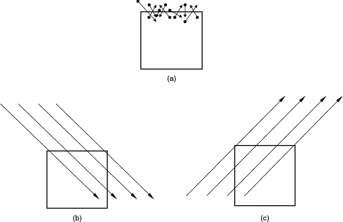
Figure 3.7.1 Transport of momentum across the top face of a small fluid parcel. (a) By molecular motions. (b) and (c) By turbulent motions, seen at different instants in time

Now consider the same mean-flow situation as we just did for the molecular shear stress, but assume that there is now also a turbulent shear stress τ_xy given by Again there is no mean velocity perpendicular to the face of our fluid parcel, but at any instant the perpendicular continuum velocity component v′ will usually be nonzero, as illustrated in Figure 3.7.1b. In these illustrations, v′ is shown as uniform over the parcel face because the parcel is assumed small compared to distances over which v′ varies. In the case of molecular transport, we had molecules crossing the face in both directions at once, arriving from very short distances since their last collisions. In the case of turbulent transport, we have macroscopic masses of fluid sloshing across the parcel face from one direction and then the other, carrying with them some “memory” of conditions where they came from, conditions that depend on the complex turbulent structures (e.g., eddies, vortices, bursts, and sweeps) of which the sloshing motion is a part. The nature of the memory that the sloshing fluid masses carry is complicated because each part of the mass has its motion modified continuously by interaction with the surrounding fluid up until the instant that that part crosses the parcel face. The distances over which the sloshing carries some influence can be as large as the thickness of the turbulent shear layer or as small as the dimension of the smallest turbulent structure, but in any case many orders of magnitude longer than a molecular mean-free-path. Thus although the Reynolds stress is a local statistical property of the turbulent motion, it depends directly on flow structure that is not only complex, but is much less local than the simple velocity gradient ∂u/∂y that determines the viscous stress.

So in the Reynolds-averaging process, we've thrown out some very nonlocal turbulence effects, and our task in turbulence modeling is to represent these effects in the context of the RANS equations, a set of local PDEs. The additional equations that are introduced in implementing various turbulence models tend to be mostly local algebraic or differential equations. Some models also include explicit nonlocal information, but generally only of a very low-level variety, such as the distance to the nearest solid surface, or some measure of the thickness of the turbulent shear layer as reflected in the mean-velocity profile. Otherwise, nonlocal effects are felt only through the behavior of turbulence-modeling variables such as “TKE,” “eddy viscosity,” “dissipation rate,” and so on, that depend on the flow solution. The local PDEs that govern the nonlocal behavior of such variables can represent only a limited repertoire of effects such as “generation,” “convection,” “diffusion,” “dissipation,” and “history” that at best are pale reflections of the complicated physics that was thrown out. This might seem like a recipe for failure, but so far, for obtaining practical predictions of turbulent flows, there seems to be no realistic alternative to this general approach to turbulence modeling. We just have to be realistic in our expectations and understand that our predictions will often be far from perfect.

Ideally, we would like a turbulence model to possess the following:

1. Universality, or the ability to reasonably represent any turbulent flow without requiring different empirical content for each category of flow;
2. Invariance, by which the model gives equivalent results regardless of the reference frame in which a problem is posed; and
3. Accuracy, sufficient for all reasonable engineering purposes.

With regard to universality, currently available models tend to do well only on relatively narrow classes of flows. Models developed to do well on boundary layers and wakes do less well on highly 3D or highly curved flows, and so forth. Some models, but not all, meet the invariance requirement. With regard to accuracy, many models do very well on simple flows such as free shear layers and flat-plate boundary layers, for which much of the models' empirical content was derived, but do much less well on flows with strong pressure gradients or flow curvature. The effects of flow separation and of three-dimensionality in boundary layers are particularly difficult to model accurately, as we'll see in Sections 4.4.2 and 8.6.2. In RANS solutions for practical flow situations, the turbulence modeling nearly always constitutes the most serious limitation on the physical fidelity of the simulation.

There are two main distinctions to be made between the various modeling strategies:

1. Whether the Reynolds stress is defined explicitly by the model (“Reynolds-stress models”), or indirectly in the form of an eddy-viscosity or mixing-length relationship (“eddy-viscosity models” and “mixing-length models”) and
2. The number and type of additional equations that constitute the model, over and above the mean-flow equations. In “algebraic” models, the additional equations are not differential (ODE or PDE). “One-equation” or “n-equation” generally refers to the number of additional PDEs in a model.

Eddy-viscosity modeling is based on an assumption proposed by Boussinesq in 1877 (see White, 1991), that the turbulent shear stress can be expressed in a manner analogous to the molecular shear stress in the NS equations, that is,

where μ_t is the “turbulent” or “eddy” viscosity. When applied to an actual flow, Equation 3.7.5 simply defines μ_t as a function of the local statistics of the turbulent motions, that is, the correlation. When used for making flow predictions, as part of a turbulence model, Equation 3.7.5 shifts the problem from that of modeling τ_t to that of modeling μ_t. The advantage of this is that μ_t can be simpler to model than τ_t, at least in the simple flows on which many models are based. A disadvantage is that there are limited regions in some flows in which the real μ_t is not well-behaved, and eddy-viscosity models will miss some of the details of such flows. Practical eddy-viscosity models are usually kept simple. For example, in 3D boundary-layer flows, where shear stresses in two directions must be calculated, the eddy viscosity is usually assumed to be isotropic, that is, the same in both directions, an assumption that is seriously violated in many flows, as we'll discuss further in Section 4.4.2.

The mixing-length assumption proposed by Prandtl (1925) is closely related and is usually expressed in terms of the eddy viscosity:

where is the mixing length. When applied to a real flow, this equation is simply a definition of the mixing length , just as Equation 3.7.5 was just a definition of μ_t. As part of a turbulence model, Equation 3.7.6 shifts the modeling problem again, from that of modeling μ_t to that of modeling . Some of the earliest modeling ideas for turbulent boundary layers were more naturally expressed in terms of than μ_t, an issue discussed in White (1991, Section 6.7).

Early mixing-length and eddy-viscosity models were cast in terms of algebraic equations and made use of rudimentary nonlocal information such as the distance to the wall and a measure of the thickness of the shear layer. In general CFD grids, such nonlocal information is not always easy to define unambiguously and can be expensive to compute. Reducing or eliminating the need for nonlocal information in more recent models has generally dictated moving from algebraic equations to PDEs.

A common strategy for generating additional equations for PDE-based models is to take “moments” of the momentum equation, that is, to take one or more of the components of the full unsteady momentum equation and to multiply each component of the equation by one of the velocity components, and to Reynolds-average the result. Depending on what combination of equations and velocity components is used, this can yield a conservation equation for TKE or a transport equation for Reynolds shear stress. The new equation is effectively an equation for the unknown second-order turbulence correlation, that is, the TKE or the Reynolds stress, but it contains new unknowns in the form of third-order correlations such as pressure-velocity correlations and triple-velocity correlations. Such new equations shift the modeling problem from that of modeling the Reynolds stress to that of modeling the third-order correlations. The process can be repeated to shift the modeling to higher orders, but there seems to be little to gain. The appearance of adding more “physics” to a model simply by adding more equations using this type of operation is an illusion. There is only one physical (vector) equation involved, and generating higher moments of it does not add physics; it is just algebraic manipulation. The only way this approach could lead to models with higher accuracy would be if the behavior of the higher-order correlations turned out to be less dependent on the particular flow situation, thus giving the model greater “universality,” but there is little evidence so far that this is the case.

Another approach that has been surprisingly successful is to invent a totally ad hoc “transport” equation for a quantity such as eddy viscosity or mixing length that is not actually governed by a physical conservation law. The model by Spalart and Allmaras (1994, the “SA model”) that is used in many RANS codes is an example of such a model, and for many types of flow, its performance is comparable to that of many more complicated models.

Viscous flows in most practical applications involve turbulence, and quantitative prediction thus requires turbulence modeling. Turbulence models and flow predictions using turbulence models will be discussed several more times in the course of the book. In Section 6.2.2, we'll look at incorporating surface-roughness effects into turbulence models; in Section 7.4, we'll use calculations made using turbulence models to illuminate several aspects of airfoil flows; and in Section 8.6.2, we'll discuss the turbulence-modeling issues related to swept wings.

3.8 Important Dynamical Relationships

In Section 3.3, we discussed the many things that can be deduced about the nature of flowfields based just on kinematics and on the fact that the velocity is a continuous vector field with only isolated discontinuities and singularities allowed in idealized models of the flow. In this section, we delve into the general relationships that can be deduced based on dynamics, with and without viscosity.

3.8.1 Galilean Invariance, or Independence of Reference Frame

Something we all take for granted as part of our Newtonian worldview is that the phenomena of fluid mechanics are physically the same, regardless of what reference frame we choose to view them in. Any fluid flow may be described with equal validity whether the reference frame is inertial (not accelerating or rotating) or is accelerating and/or rotating. Of course, this idea applies to classical mechanics in general, and a formal justification of it requires knowledge of Newton's laws. But there was some intuitive realization of it before Newton, as for example in the writings of Galileo and Leonardo da Vinci (see Anderson, 1997, p. 24).

For most work in fluid mechanics we use an inertial reference frame. How the idea of independence of reference frame is reflected in the mathematics in this case is worth at least a cursory look. First, the NS equations and the general statements of the BCs used with them are invariant under Galilean transformation, which means that the forms of the equations and BCs are unchanged by a transformation from one inertial frame to another. However, the phenomena the equations represent are not invariant in the same sense. They don't look the same in different reference frames; they are just physically equivalent when the effects of the different viewpoints have been accounted for. What we mean by “accounted for” is that things have been appropriately transformed in going from one frame to another. The descriptions of the same flow in two different reference frames are transformed versions of each other. So while the equations are invariant, the flowfields they govern, which are solutions to the equations, are merely transformable.

In some applications such as propellers or other turbomachines, the flow may be steady and simpler to describe in the reference frame of the rotating object. Then the effects of the rotating reference frame must be accounted for in the equations by inclusion of appropriate rotation terms. The equations are not invariant with respect to the rotational motion of the reference frame, but they can be transformed to account to the rotational motion.

The fact that we can look at aerodynamic phenomena in different reference frames and know that they are effectively the same comes in handy in many ways. For example, it is basic to the similarity between wind-tunnel testing and flight. We'll look at other aspects of dynamic similarity in Section 3.9. And in developing physical understanding, it is often helpful to look at different aspects of a phenomenon in different reference frames.

3.8.2 Circulation Preservation and the Persistence of Irrotationality

In Section 3.3.5, we defined the circulation as the line integral of the velocity around a closed contour and saw that it is equal to the total vorticity piercing any capping surface bounded by the contour, by virtue of Stokes's theorem. The circulation can reflect the dynamics in ways that make it a useful quantity in numerous situations; for example, as we'll see in Section 7.2, it is related to lift through the Kutta-Joukowski theorem.

It is often useful to be able to make general statements about whether circulation is preserved or not. Considering the circulation around a closed material contour that moves with the flow, under what conditions can we expect that it is preserved, that is, that it remains constant in time? In other words, under what conditions is the Lagrangian rate of change of the circulation equal to zero? This can be written as

Note that we can reverse the order of differentiation and integration in Equation 3.8.1, so that it becomes the statement that the line integral of DV/Dt around a closed contour is zero, which is true only if DV/Dt is the gradient of a scalar function, called an acceleration potential. (See the analogous argument in Section 3.3.6 regarding the velocity potential in irrotational flow.) By invoking the momentum equation, we can show that this requires:

1. No net viscous force on any fluid parcel on the contour. This requires either that the viscosity is zero, or that the fluid is uniform and the flow is irrotational. But the second of these options is of little interest, because requiring irrotationality means that Equation 3.8.1 is satisfied trivially.
2. Any external body force is the gradient of a potential, such as gravity.
3. The fluid is barotropic, that is, the density is a function of pressure only. This is commonly satisfied only if the fluid is homocompositional and entropy is constant in the flowfield, conditions that in aerodynamics often apply to inviscid flow in the absence of shocks. But zero viscosity is not strictly required for this condition to be met. A uniform fluid meets this requirement by definition, even if it is viscous.

This result is sometimes referred to as Kelvin's circulation theorem. In some references (for example, Milne-Thomson, 1966), condition 3 is not mentioned explicitly, but it is still implicitly assumed.

Circulation preservation of this kind supports the persistence of irrotationality in many situations. This is easy to see if we think of a flow that starts out irrotational, say upstream of its approach to a body or other source of disturbance. In this initially irrotational state, the circulation must be zero around any reducible closed contour. Then if the flow is circulation preserving, any circulation must remain zero as the flow progresses. The vorticity must also remain zero, since if any nonzero vorticity appeared, there would be nonzero circulation around some closed contour, which would violate our assumption of circulation preservation. So circulation preservation means that a flow that starts out irrotational will remain irrotational downstream.

Preservation of irrotationality is especially simple in the special case of a uniform fluid (constant density and viscosity). A uniform fluid satisfies condition 3 above by definition, and an irrotational flow of a uniform fluid produces no net forces on fluid parcels even if the viscosity is nonzero (see Section 3.6), so that it also satisfies condition 1. For the kinds of compressible flows we are likely to encounter in practice, variations in fluid properties tend to be slow enough that condition 1 is effectively, though not exactly, satisfied in regions of irrotational flow, and condition 3 is satisfied in regions where the flow is isentropic.

In Section 3.6, we discussed the general flow pattern that characterizes external flow past bodies at high Reynolds numbers (small viscosity), in which a vortical boundary layer develops close to the body surface, surrounded by essentially irrotational flow that behaves as if it were inviscid. What we have seen here regarding the persistence of irrotationality is consistent with that picture. Ordinarily, you should expect that when the flow approaching a body from upstream is irrotational, significant vorticity will appear in the flowfield only where it has diffused and convected from the body surface or where it has been produced by a strong, curved shock (see Crocco's theorem, Section 3.8.5 and the discussion of shocks in Section 3.11).

3.8.3 Behavior of Vortex Tubes in Inviscid and Viscous Flows

In Section 3.3.7, we introduced the concepts of vortex tubes and vortex filaments, and we saw that the intensity of a vortex filament is constant along its length (Helmholtz's second theorem). By noting that we can consider a vortex tube as a bundle of vortex filaments, we can define the intensity of a vortex tube as the sum of the intensities of the filaments within the tube. (For a vortex tube of finite cross section, this “sum” is actually an integral, because vortex filaments are of infinitesimal size.) Now we assume that the flow is circulation preserving in the sense defined in Section 3.8.2, that is, that the conditions for Kelvin's circulation theorem are met. In this instance, we are by definition concerned with flows with nonzero vorticity, so the only option that satisfies condition 1 for circulation preservation is for the fluid to be inviscid. Then two dynamics-based theorems apply:

Helmholtz's third theorem: As a vortex tube evolves in time, fluid parcels cannot cross the bounding surfaces of the tube, and as a result the tube is always made up of the same fluid parcels.

Helmholtz's fourth theorem: The intensity of a vortex tube is constant regardless of how the tube moves around.

A proof that makes use of Stokes's theorem is given by Milne-Thomson (1966). In a rigorous sense, it might seem that these two theorems are not very informative or useful, because they deal with vorticity in inviscid flows, while in most cases of interest in aerodynamics the only way for vorticity to be there is through the effects of viscosity. But if we view the inviscid case to which they apply as being the limiting case for flows with small viscosity, we can get some useful insight from them. Basically, what Helmholtz's third theorem tells us is that for small viscosity, the natural tendency of a vortex tube is to remain anchored to the same material tube, and that vorticity migrates into or out of that material tube only through viscous diffusion. In Section 3.6, we discussed the vorticity equation and the transport of vorticity by convection and diffusion. Helmholtz's third theorem provides further insight into what it means for vorticity to be transported mainly by convection. Helmholtz's fourth theorem tells us something that's a bit harder to visualize: that vorticity migrates into or out of a vortex tube only by viscous diffusion.

The assumption of small viscosity is not always as limiting as it might seem. Nearly all of the vorticity in aerodynamic flows is generated at solid surfaces, and in the thin viscous or turbulent boundary layers on those surfaces, the effects of viscosity are not small. So in these parts of the flow, the insights provided by these theorems are not very applicable. But when the vorticity is convected into the wake away from the body, the viscous and turbulent stresses are rapidly reduced, and the above insights become more useful, as, for example, in Section 8.1, when we consider the vortex wake behind a 3D wing.

3.8.4 Bernoulli Equations and Stagnation Conditions

We've seen that effectively frictionless flow conditions are frequently encountered in practice, particularly outside the viscous boundary layer that develops near the surface in flows around bodies. Under these conditions, with a couple of additional restrictions, Bernoulli's principle defines a simple relationship between the pressure and the velocity magnitude. This is analogous to the many situations in classical particle mechanics in which the total force exerted on a particle can be expressed as the gradient of a potential that is a function of position only, a condition that often applies in the absence of friction effects. In these situations, the sum of the “potential energy” and kinetic energy is constant, which leads to a simple relation between the potential function value and the particle's velocity magnitude.

To determine the requirements for the analogous situation to exist with regard to the net force on a fluid parcel, we can either look directly at the energy equation or take a line integral of the momentum equation. Either way, we find that if:

1. There is no net viscous force on fluid parcels;
2. external body forces are negligible;
3. there is no heat conduction; and
4. the flow is steady,

then the total enthalpy

is constant along streamlines, where e is the thermodynamic internal energy per unit mass. Note that under these conditions p/ρ acts like a form of potential energy. Note also that conditions (1) and (3) amount to specifying the absence of entropy-generating processes (assuming bulk-viscosity effects are also negligible), so that entropy must also be constant along streamlines.

Now we introduce the concept of stagnation conditions, which can be defined for general flows that don't necessarily satisfy the assumptions for Equation 3.8.2. From any point in a general flow, we can imagine bringing the fluid parcel passing that point to rest (stagnation, or zero velocity) by an imaginary steady-flow process in which the viscous forces and heat conduction that may be active in the general flow are “turned off” and for which Equation 3.8.2 therefore applies. Because the imaginary stagnation process is isentropic, the stagnation values of T, p, and ρ are uniquely defined, and we'll designate them by the subscript t for “total.” In general flows, these stagnation conditions need not be constant, either along or across streamlines. It is important to keep in mind that the stagnation temperature, pressure, or density is not generally a real temperature, pressure, or density, but is only an imaginary construct defined by an imaginary process. The exception is a real stagnation point in a steady flow, where the stagnation condition can actually be realized.

Returning our attention to flows that satisfy Equation 3.8.2 and introducing stagnation quantities, Equation 3.8.2 becomes

along streamlines, where all of the subscript t quantities are constant along streamlines as well. Now if we assume a perfect gas and impose the constant-entropy condition, we have

and

so that Equation 3.8.3 becomes (see National Advisory Committee for Aeronautics (NACA) Report 1135, Ames Research Staff, 1953)

along a streamline, where the subscript t quantities are constants for that streamline. We'll call this the steady, compressible Bernoulli equation for frictionless, nonconducting flow of a perfect gas. If the density is constant, that is if the flow can be assumed effectively incompressible, in that the density change in response to any pressure change in the flowfield is a sufficiently small percentage (see Section 3.10), this reduces to

along a streamline.

To recap, the Bernoulli principle can be simply stated: For steady, frictionless flow with no body forces and no heat conduction, the total enthalpy is constant along streamlines. Because such flows are also generally isentropic along streamlines, the total pressure and temperature are also constant along streamlines. How the “Bernoulli constant” and the stagnation conditions vary from streamline to streamline, however, depends on how the flow was established, which brings us to our next topic.

3.8.5 Crocco's Theorem

Assume that a flow satisfies the conditions given above for the Bernoulli principle to apply, so that Equation 3.8.2 holds along streamlines. If we assume further that the fluid is homo-compositional, that is, that it consists everywhere of the “same stuff,” as would be the case if the relative species concentrations in a mixture of gasses were constant, then a standard thermodynamic relationship between T, S, e, p, and ρ (one of the familiar “TdS” or “tedious” equations, see Liepmann and Roshko, 1957) applies throughout the flowfield. Combining this with the momentum equation (remember that the flow is assumed steady and frictionless), we get

which is known as Crocco's theorem.

We saw earlier that it is common in external flows around bodies for the flow to be “established,” that is, to come from upstream, in an irrotational state. If it continues to satisfy the requirements for Crocco's theorem to apply in the part of the flowfield outside the viscous boundary layers near the body surface, the flow will remain irrotational, in which case we can see that constant H implies constant S and vice versa. Thus in the effectively inviscid parts of many external flows, the total enthalpy, our “Bernoulli constant,” will usually be constant from streamline to streamline, as well as along streamlines. If such a flow passes through a curved shock (see Section 3.11.2), however, the situation downstream of the shock will be more complicated. The portions of the shock through which different streamlines pass will have different obliqueness, and S will therefore vary from streamline to streamline, though H will still be constant. In Equation 3.8.8, the RHS will be zero, and the varying S will require nonzero vorticity. Thus a curved shock inevitably produces some vorticity downstream, though it is typically very weak unless the shock is very strong.

For a more detailed discussion of circulation preservation, Bernoulli's principle, and Crocco's theorem, readers would do well to consult Chapter 3 of Batchelor (1967). I hope those who do will accuse me at worst of oversimplifying and not of plagiarizing.

3.9 Dynamic Similarity

Using flows around subscale models to simulate what would happen at full scale has been a major tool in aerodynamic development since the Wright brothers built their first wind tunnel. Subscale model testing has made it practical to explore many more design options and a wider range of flight conditions than could be explored by flight testing alone, and the savings in time, money, and test pilots' lives have been incalculable. Advances in CFD in recent years have made it possible for CFD to replace some subscale model simulation, but it will be a long time before computation replaces all of it.

In practice, the similarity between a subscale flow simulation and the real thing is rarely even close to perfect. However, defining the theoretical requirements for a perfect simulation will tell us what factors are important and provide at least some basis for anticipating how accurate our actual simulations are likely to be.

A perfect simulation requires that the model geometry and the model flow be geometrically scaled versions of the real things, with all of the detailed forces and accelerations and other internal processes reproduced in a properly scaled fashion. Presumably if we knew everything we needed to know to be able to set up such a simulation correctly, we would also know the scaling factors for converting quantities such as pressures and integrated forces from model scale to full scale. The early pioneers were able to deduce some of the important scaling factors from a combination of intuition and experience, such as the scaling of forces with surface or cross-sectional area times the square of the velocity, but they were not always aware of the more subtle requirements for similarity. With our advanced understanding of the governing equations, we are in a position to derive these requirements with some rigor.

The basic idea is that if we “nondimensionalize” the governing NS equations and BCs appropriately for both situations (model and full scale), the two flows will be similar if they represent the same solution to the dimensionless equations. Of course, this can be expected to happen only if the dimensionless equations themselves, and the dimensionless BCs, are the same for both situations. This sounds simple enough, but there are subtleties involved, as we'll see below.

To derive the dimensionless equations, we start by replacing each dimensional quantity in the equations with a product of a dimensional reference constant and a dimensionless version of the original variable. The reference constants are simply quantities appropriate to the flow situation, such as freestream flow properties (e.g., velocity and density) and a reference length that characterizes the body, and we naturally have to use equivalent definitions for these constants for both flow situations. We make these substitutions likewise for all of the independent spatial coordinates and all of the dependent flow variables. Then for each equation, we choose a group of the reference constants having the right combined dimensions so that when we divide the entire equation by that group, the equation becomes dimensionless. There is no unique right choice of the group of constants to use for this nondimensionalizing step, but the resulting equations are of course equivalent, no matter what group is chosen.

The conventional choice is based on the observation that inviscid flows have no inherent scale dependence, and that it is therefore convenient to choose the nondimensionalizing group so that the nonviscous terms in the dimensionless equations end up looking just as they do in the original equations, with no scale-dependent coefficients multiplying them. For the momentum equations, this means dividing by , and for the energy equation in total-enthalpy form by u_ref p_ref/L_ref. In our final set of dimensionless equations, the nonviscous convective terms look the same as they did in the dimensional equations, while the pressure gradient, viscous-transport, and heat-conduction terms have dimensionless “scaling” or “similarity” parameters multiplying them.

Now we see that for the dimensionless equations to be the same for both the simulation and for full scale, the similarity parameters multiplying the pressure and transport terms must have the same values in both cases.

Now let's look specifically at the dimensionless parameters that arise. We form dimensionless versions of all the basic variables in the equations, designating them by putting “hats” over them. We nondimensionalize the basic variables as shown in Table 3.9.1.

We invert these definitions (e.g., ) and substitute them into the form of the equations valid for a perfect gas with constant specific heats. We also make use of the specific heat relationship c_p = γR/(γ − 1), where γ is the ratio of specific heats and R is the gas constant, and of the fact that the speed of sound is given by a = (γp/ρ)^1/2. In the resulting dimensionless equations, the continuity equation and the convective terms in the momentum equation and in the energy equation in total-enthalpy form look exactly as they did in the original dimensional equations. Terms in which dimensionless similarity parameters appear are as shown in Table 3.9.2, where M_∞ = u_∞/a_∞ is the freestream Mach number, R_L = ρ_∞u_∞L/μ_∞ is the Reynolds number, and Pr = μc_p/k is the Prandtl number.

Based on this, we might expect perfect similarity if we match γ M_∞², R_L, and Pr. But things aren't quite so simple with regard to γ and M_∞. One of our primary variables in the energy equation is , which is defined in terms of other dimensionless variables as

Table 3.9.1 Basic variables

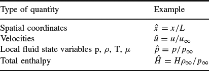
Table 3.9.2 Terms appearing in dimensionless equations

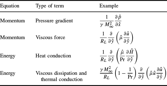
So the internal energy (first term) and kinetic energy (second term) in the total enthalpy depend on γ in different ways, and true similarity requires that we match γ and M_∞ separately.

To summarize, similarity parameters that must be matched for perfect similarity are:

Ratio of specific heats	γ = cp/cv
Mach number	M∞ = u∞/a∞
Reynolds number	RL = ρ∞u∞L/μ∞
Prandtl number	Pr = μcp/k

Note that some of these are fluid properties (γ and Pr) and some (M_∞ and R_L) depend in addition on the reference flow conditions, in this case the far field. Now let's consider the major scaling and similarity issues in detail: compressibility effects, the effects of viscosity, scaling of pressure forces, and the consequences of failing to match the similarity requirements.

3.9.1 Compressibility Effects and the Mach Number

Throughout the flowfield the interaction between the pressure and density for compressible flows is governed by implicit relationships built into multiple equations, and γ and M_∞ correspondingly appear in several places. We saw above that similarity requires us to match γ and M_∞ separately.

Of the flow-dependent parameters, Mach number has the most straightforward physical interpretation. It determines how large the pressure changes in the flowfield will be, relative to the absolute pressure, and thus how important pressure-induced density changes will be, a topic we'll consider further in Sections 3.10 and 3.11. The Prandtl number is important with regard to thermal effects in boundary layers, and we'll consider it further in Section 4.6.2.

3.9.2 Viscous Effects and the Reynolds Number

The Reynolds number is also widely familiar, but its proper interpretation is more subtle. Reynolds number is sometimes described as measuring the “ratio of inertial forces to viscous forces,” which is incorrect, or the “relative importance of inertial forces and viscous forces” in the flow, which is not as bad, but not quite right either. Actually, the term 1/R multiplies the viscous terms in the momentum and energy equations, but it does not directly reflect the relative magnitudes of the forces locally. In any external flow with a Reynolds number above about 10², there will be part of the flow outside the boundary layer where the ratio of inertial forces to viscous forces will be practically infinite and part of the flow deep in the boundary layer where it will be practically zero. Thus the ratio of local forces is obviously not what the Reynolds number directly determines.

What the Reynolds number does determine is how “fast,” relative to the flow velocity, momentum will be diffused in the cross-stream direction by viscosity or turbulence and thus how thick the boundary layer will grow relative to the dimensions of the body. As Reynolds number increases, the diffusion of momentum becomes relatively slower, and the boundary layer will be thinner. This increases the velocity gradient inside the boundary layer, which offsets the reduction in the 1/R multiplier in front of the viscous terms. The result is that the variation across the boundary layer in the relative importance of viscous forces stays essentially the same, regardless of the Reynolds number: At the “bottom” of the boundary layer, viscous and pressure forces dominate, while at the “edge” of the boundary layer viscous forces are small, and inertial and pressure forces dominate. Thus the idea that the Reynolds number measures “relative importance” makes sense only if we apply it to global viscous “effects” as opposed to local viscous “forces.” As the Reynolds number increases, the boundary layer becomes thinner and has less effect on the rest of the flow. It is only in this indirect sense that the Reynolds number measures the relative importance of viscous effects.

We've just used a simple physical argument to explain why the effects measured by the Reynolds number are subtle. The corresponding mathematical argument is less intuitive and starts with the observation that the viscous terms involve the highest order derivatives of the velocity and therefore play a unique role in the equations. If we set 1/R to zero, the viscous terms vanish, and we have the inviscid equations. We might expect, then, that for small values of 1/R, a viscous solution could be obtained as a small perturbation to a corresponding inviscid solution. This expectation is wrong, however, because when the 1/R terms are dropped to obtain the inviscid equations, the order of the equations is reduced, and with it the number of allowable BCs. The BC we must give up to allow nontrivial inviscid solutions is the no-slip condition. To obtain a viscous solution from the corresponding inviscid solution, the no-slip condition must be reinstated, and there will always be a region close to the wall (the boundary layer) where the perturbation imposed on the inviscid solution by viscosity is not small. In mathematical terms, this is an example of a singular perturbation, and the kind of behavior we've been discussing is characteristic of singular-perturbation problems. In Section 4.2.1, we'll discuss how the implementation of the singular-perturbation idea leads to a rigorous derivation of boundary-layer theory.

So far, we've seen that the way the characteristics of a flow depend on the Reynolds number is complicated by the fact that a change in the 1/R multiplier in front of the viscous terms tends to be offset by a change in boundary-layer thickness. This complication is compounded by additional subtleties. The location on the body where the boundary layer transitions from laminar to turbulent usually depends on Reynolds number, and this can strongly affect the development of the boundary layer and thus the rest of the flow. Though the variation of boundary-layer thickness with Reynolds number in laminar and turbulent boundary layers is similar qualitatively, it is significantly different quantitatively. The location of laminar-to-turbulent transition strongly affects both the profile drag in the attached-flow regime and the resistance of the boundary layer to separation downstream. Such effects can be very important in airfoil flows, as we'll see in Section 7.4, and in bluff-body drag, which we'll discuss in Section 6.1.6.

3.9.3 Scaling of Pressure Forces: the Dynamic Pressure

When we divide the momentum equations by , the resulting dimensionless convection terms look just as they did in their original dimensional form. For example, the original dimensional term

becomes

where , ,

When we nondimensionalized the equations to derive the similarity parameters, we nondimensionalized p by p_∞. But this nondimensionalization of the pressure isn't very convenient for dealing with low-speed flows. If, instead, we take our reference pressure equal to what is called the dynamic pressure , the original dimensional pressure-gradient term:

becomes

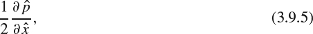
where . We introduced the factor of 1/2 in the definition of our reference pressure because it arises when we integrate the momentum equation to obtain Bernoulli's equation, as we saw in Section 3.8.4, and q defined in this way is equal to the difference between local static pressure and total pressure in the incompressible, or low-Mach-number case, as in Equation 3.8.7. (A discussion of what “incompressible” means is coming up in Section 3.10.)

Normalizing pressure differences by q is very convenient because it removes the dependence on density and velocity in incompressible flows, and it has therefore become second nature to aerodynamicists. And q is used as a reference for compressible flows as well, though outside of the low-Mach regime, it no longer removes all of the dependence on velocity, or Mach number.

3.9.4 Consequences of Failing to Match All of the Requirements for Similarity

In most subscale flow simulations we must tolerate a substantial mismatch in one or more of the similarity parameters. How does the accuracy of a simulation suffer as a result? In this regard, the first thing to note is that the parameters are not all of equal importance and that their relative importance depends on the situation.

In flows with sufficiently low Mach number throughout the field, matching Mach number is not important, while in flows where local Mach numbers approach or exceed one, matching Mach number is crucial. Fortunately, Mach number is formally scale independent and therefore relatively easy to match regardless of scale. In cases where Mach number is important, we can usually avoid having to tolerate a serious mismatch.

Unfortunately, we can't say the same of the Reynolds number, which varies directly with scale. For a given flow condition, a reduction in scale (our main reason for doing subscale simulation) entails a reduction in Reynolds number. Testing at elevated pressures can alleviate the problem but can't generally eliminate it. At high subsonic speeds, testing at total pressures above about 5 atm is impractical because air loads on a typical airplane model become too high, even for a model constructed of solid steel. The only way the full-scale Reynolds number of a large airplane can be matched on a small-scale model in a wind tunnel is through a combination of elevated pressure (up to 5 atm) and very low temperature (to −250 °C), called cryogenic pressure testing.

Such testing is very expensive and accounts for only a miniscule fraction of all wind-tunnel flow simulation. Most other subscale testing is done at Reynolds numbers roughly an order of magnitude below full scale. As we saw previously, the dependence of a flow on the Reynolds number is complicated, with contributions from a number of physical factors. The sacrifice in simulation accuracy due to a mismatch in the Reynolds number varies greatly depending on the situation, but it is usually serious. A great deal of work has been devoted to the problem of understanding, minimizing, and accounting or correcting for the “Reynolds-number effects” associated with testing at sub-full-scale Reynolds numbers, with mixed success (see Bushnell, 2006, for a review).

In our derivation of the terms in which similarity parameters appear (Table 3.9.2), we assumed a perfect gas. The idea of a perfect dynamic similarity is problematic if we consider the more complicated behavior of real gases over wide ranges of conditions. In the general case, the pressure and temperature, as well as the composition of the gas, would have to be matched, in which case there could be no difference in density, and no difference in scale would be allowed. Fortunately, air under conditions of interest to us in aerodynamics behaves very much like a perfect gas, with practically constant γ and Prandtl number, so that mismatches in parameters other than the Mach and Reynolds numbers tend to have very minor effects (see White, 1991). For example, because of the nonlinear form of the Sutherland law for the dependence of viscosity on temperature, perfect similarity would require matching temperature. However, because the temperature variation within a given flow is usually not large on an absolute scale, the effect of even a large mismatch in temperature at a given Reynolds number is very small.

3.10 “Incompressible” Flow and Potential Flow

In early theoretical work in fluid mechanics, the fluid was generally assumed to have constant density regardless of the pressure, and thus to be “incompressible,” an idealization that greatly simplifies the mathematics and is actually justified at sufficiently low Mach numbers. The term “incompressible,” however, is a potential source of confusion. Literally speaking, saying that something is “incompressible” means that it cannot be compressed. In this sense, the term is only approximately applicable to liquids and not at all applicable to gases. Yet even with reference to gases, we often talk loosely about “incompressible flow.” This is sloppy terminology. We don't mean what the term literally says (i.e., that the flow cannot be compressed). What we really mean is that the flow happens not to be getting compressed significantly in this particular situation and that it therefore behaves as if it were incompressible.

In gases at low Mach numbers, a flow can act as if it were incompressible, in that we can make very accurate predictions using equations in which we have assumed that the density is constant. But how can constant density be a reasonable assumption for gases, which are by definition highly compressible? Even in flows at low Mach numbers, where velocity differences, pressure differences, and density differences are all small, the density differences are of the same order as the pressure differences. How can the pressure changes be important and the density changes not be? The answer lies in the different roles that pressure and density play in affecting the motion. In the application of Newton's second law to a fluid parcel, only a pressure difference can apply an unbalanced force, while the density itself provides the resisting inertia. In the momentum equation, this is reflected in the fact that the pressure appears inside a derivative (gradient operator), and the density does not. While the small velocity and pressure differences are crucial players in the momentum balance, the small density differences have a comparatively much smaller effect on the flow.

Note that to justify treating the flow as incompressible we do not have to assume small disturbances in the sense of small velocity changes relative to the freestream velocity. The changes in velocity can be large relative to freestream, as long as the velocity itself remains small relative to the speed of sound.

So the equations of motion for an “incompressible” fluid are valid for flows of highly compressible gases, in the limit of low Mach number. If we also assume that the flow is steady and inviscid, and that the onset flow is irrotational, we have met the conditions for classical potential flow or ideal flow theory. As we saw in Section 3.8.2, a constant-density inviscid flow is circulation preserving, so that irrotational onset flow means the flow will be irrotational everywhere. Then, as we saw in Section 3.3.6, the velocity field can be represented as the gradient of a scalar potential function:

and the continuity equation is Laplace's equation for ϕ:

Assuming the pressure is related to the velocity by the “incompressible” Bernoulli equation (Equation 3.8.7) with a constant total pressure, any flow that satisfies Equation 3.10.2 satisfies both the continuity and momentum equations. Under these conditions, the energy equation is not needed, and Equation 3.10.2 with appropriate BCs represents the complete system describing the inviscid, irrotational flow of a constant-density fluid. The problem has been reduced to a single linear equation with a single scalar as the dependent variable.

Because the incompressible potential-flow equation is linear, solutions can be constructed by superposition of more than one known solution. The velocity potentials for elementary building-block flows around simple singularities are often used for this purpose. Some examples are illustrated in Figure 3.10.1. A vortex Figure 3.10.1a can be used to produce circulation, and sources or sinks Figure 3.10.1b can be used to simulate the thickness effect of a body. The combination of a source and sink of equal strength results in flow pattern Figure 3.10.1c. In the limit as the separation distance between them goes to zero, keeping the product of the source/sink strength and the separation distance constant, we have a doublet Figure 3.10.1d. Combining a doublet with a uniform flow produces a pattern Figure 3.10.1e in which the outer part is the potential flow around a circular cylinder. And many other combinations are possible.

For 2D flows, conformal mapping provides solutions for flows over convex and concave corners. Knowing the character of these solutions is useful just for thinking about the local effects of corners in general, and in Section 4.3.2 we'll see that they provide the outer-flow BCs for a family of special solutions to the boundary-layer equations. The basic idea is that a simple analytic mapping can transform the x axis into a line that is bent at the origin through an angle πβ/2. The uniform flow in the upper half plane, illustrated in Figure 3.10.2a, is then transformed into corner flows like those illustrated in Figure 3.10.2b–d. The velocity distribution along the surface is given by u ~ x^m, where m = −β/(β − 2).

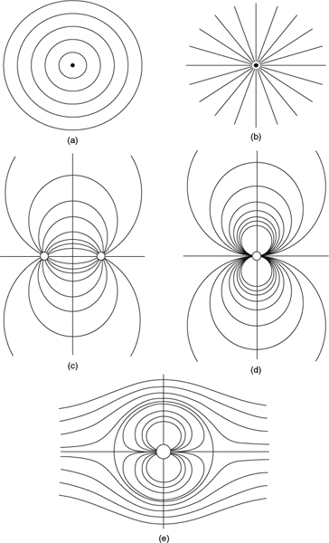
Figure 3.10.1 Examples of streamline patterns associated with simple potential-flow singularities that can be used in constructing other potential-flow solutions by superposition. (a) Vortex. (b) Source or sink. (c) Combination of source and sink of equal strength. From Durand, (1932). Used with permission of Dover Publications, Inc. (d) Doublet. From Durand, (1932). Used with permission of Dover Publications, Inc. (e) Combination of a doublet and a uniform flow yielding a circular cylinder. From Durand, (1932). Used with permission of Dover Publications, Inc.

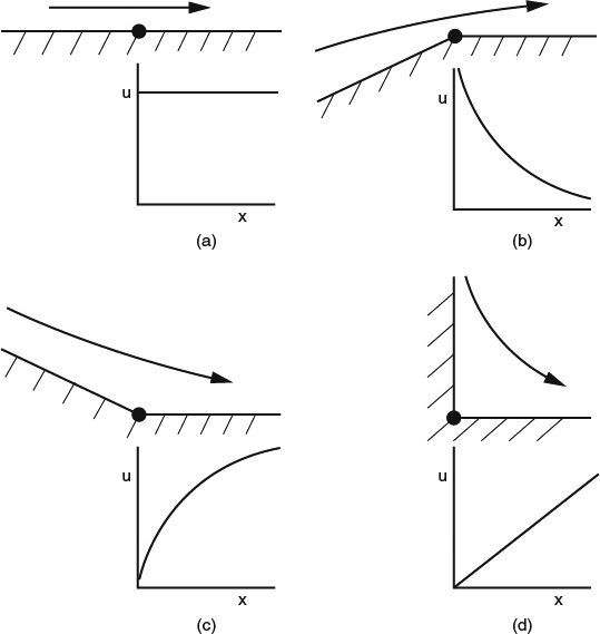
Figure 3.10.2 Illustrations of potential flows over concave and convex corners that can be produced by conformal mapping of the uniform flow in the upper half plane. (a) Uniform flow. (b) A convex corner: −1 < β < 0. (c) A concave corner: 0 < β < 1. (d) A 90-degree concave corner: β = 1

Velocity distributions that go with the different types of corners are illustrated in Figure 3.10.2. In Figure 3.10.2b, we see that a convex corner produces infinite velocity at the corner and decelerating flow away from it. In Figure 3.10.2c, a concave corner produces zero velocity (a stagnation point) at the corner. Combine this flow with its reflection about the x axis, and we have the flow off of a wedge-shaped trailing edge. This demonstrates that in potential flow, an airfoil with a nonzero trailing edge angle must have a trailing-edge stagnation point. In Figure 3.10.2d, we have the special case of β = 1, a 90° corner with a stagnation point and linear acceleration of the flow away from the corner. Combine this flow with its reflection about the y axis, and we have the prototype for flow attaching itself to a smooth wall at a stagnation point. Conformal mapping can also be used to transform solutions for very simple shapes such as circles into solutions for more-complicated shapes. With the conformal-mapping approach, analytic solutions are possible for a wide variety of shapes.

We can obtain numerical solutions for 2D flows either by discretizing the conformal-mapping problem or by the “panel method,” that is solving for a distribution of unknown singularity strength along a set of discrete panels representing the body surface. When the panel method is extended to 3D flows, not only the surface of the body must be “paneled,” but also any vortex wakes that exist in the field, which, as we saw in Section 3.3.8, can be idealized as surfaces of discontinuity in the velocity field.

As we saw in Sections 3.6 and 3.8.2, external flows around bodies at high Reynolds numbers remain effectively irrotational outside of a thin viscous boundary layer that develops near the surface. Potential flow is therefore not a bad approximation for many of these flows and can often provide very reasonable predictions of pressure distributions and integrated forces at low Mach numbers. The pioneers of theoretical aerodynamics took full advantage of this, and before large-scale computation of nonlinear flow problems became practical, much of our quantitative prediction capability depended on incompressible potential-flow theory, most often implemented in the form of panel methods. It remains a powerful tool both for conceptualizing and for quantitative calculations.

3.11 Compressible Flow and Shocks

“Compressibility” deals with changes in fluid density in response to changes in pressure. In the previous section, we discussed how these changes are insignificant at low Mach numbers. As Mach number increases, however, we can no longer ignore the density changes, and when the local Mach number exceeds one, their effects on the flowfield become so strong that the character of the flow changes drastically, as reflected for example in the response of the flow to changes in cross-sectional area, which is essentially reversed between the subsonic and supersonic regimes.

There are small-disturbance flow regimes, both subsonic and supersonic, in which the effects of compressibility are treated approximately, in the context of linear equations. These theories have such narrow ranges of applicability, however, that they are usually not very useful, and they have been marginalized in recent years by the availability of higher-fidelity computational methods. We'll touch on the linear theories again in Chapter 9 when we survey broad classes of theoretical approximations. In this section, we explore what happens when we attack the problem of compressibility head on, without assuming that disturbances are small.

In compressible flows, the changes in density bring with them changes in local temperature and in all of the fluid properties that are affected by temperature. These changes have significant local effects on the flow, and accurate flow prediction requires solving for the altered local fluid properties in detail. As we discussed in Section 3.1, the viscosity, thermal conductivity, and local speed of sound are usually assumed to depend on temperature only.

A general feature of most transonic and supersonic flows is the appearance of compression shocks, regions in which significant amounts of deceleration and compression (pressure increase) take place over very short distances, on the order of the mean free path of the gas molecules. The extremely large gradients inside a shock are beyond the strict range of validity of the NS equations. As we've already noted in Section 3.1, the NS equations don't predict the internal structure of a shock accurately, but because the equations also enforce the integrated conservation laws, they do capture the “jump” conditions across shocks correctly. Shocks tend to form in most transonic and supersonic flows because sustained deceleration and compression in supersonic regions is usually not possible, especially when the deceleration goes all the way from supersonic to subsonic. There are exceptional situations in which sustained gradual deceleration can occur, but they are not common in practical situations. In most ordinary situations, infinitesimal compression waves in a supersonic region tend to pile up on each other and to coalesce into a shock. Details on this process can be found in Shapiro (1953) or Liepmann and Roshko (1957).

Shocks in steady flows can be locally perpendicular (normal) or oblique to the flow. Figure 3.11.1 illustrates several examples of steady flowfields with shocks. In Figure 3.11.1a we have a transonic airfoil flow, with a “bubble” of supersonic flow over the upper surface, terminated by a weak shock that is generally curved and slightly oblique. This global flow pattern is typical of jet airliner wings in high-speed subsonic cruise (The simplified sketch omits the details of the interaction between the shock and the boundary layer, which we'll discuss in Section 7.4.8). In Figure 3.11.1b we have flow over a sharp wedge or cone at a sufficiently high supersonic freestream Mach number to produce an attached oblique shock propagating from the nose. In this case, the flow downstream of the shock is still supersonic. In Figure 3.11.1c we have supersonic freestream flow past a blunt-nosed body with a detached, curved bow shock standing off the nose. In this case, there is a “bubble” of subsonic flow downstream of the part of the shock that is close to normal, and supersonic flow downstream of the more oblique parts of the shock. Of course, more complicated patterns are possible, especially in 3D, with shocks from different parts of a body intersecting, or with shocks being affected by expansion waves from other parts of the body. In Section 3.11.2, we'll discuss the local relationships the flow through a shock must obey.

With or without shocks, compressible flow is inherently more complicated than incompressible flow. The full system of equations for compressible flow, even if assumed inviscid, is nonlinear and entails all the difficulties we discussed in Section 3.5. Except for a very few simple cases, analytic solutions for flows in more than one dimension are not possible, and the prediction of a multidimensional flowfield generally requires large-scale computation.

But all is not lost. There is still a great deal that can be learned about steady multidimensional compressible flows without resorting to computation, based on the combination of continuous 1D flow theory and the relations governing normal and oblique shock waves. Most real flows are not close to being 1D, and the 1D flow theory/shock relations are therefore not globally predictive, but they are still powerful tools because they provide simple ways to calculate useful relationships between the various flow quantities, applicable along streamlines of steady multidimensional flows. Their general usefulness is thus analogous to that of Bernoulli's equation for incompressible flow.

3.11.1 Steady 1D Isentropic Flow Theory

If the flow is steady, the flow in any given slender streamtube in a flowfield is effectively 1D. If we assume that the flow is inviscid and isentropic, as it usually would be outside the boundary layer near solid surfaces, and that the fluid is a perfect gas, then the 1D equations of motion can be integrated analytically. Note that these assumptions satisfy the requirements for the compressible Bernoulli equation (Equation 3.8.6) to hold, so that stagnation conditions are constant along our streamtube. Remember also that if we further assume that the fluid is homocompositional, such that Crocco's theorem (Equation 3.8.8) holds, and that the onset flow is irrotational, then the stagnation conditions will be the same in all of the streamtubes in the field, at least upstream of all shocks. Downstream of any shock, the stagnation pressure is reduced, as we'll see next.

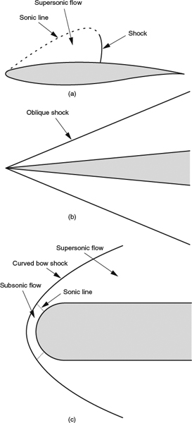
Figure 3.11.1 Examples of flowfields with compression shocks. (a) A transonic airfoil flow with a bubble of supersonic flow over the upper surface, terminated by a shock. (b) Supersonic flow over a sharp wedge or cone, with an attached oblique shock. (c) Supersonic flow over a blunt-nosed body with a detached bow shock

The result of the steady 1D flow theory for a perfect gas is a set of relationships defining dimensionless ratios of flow variables. This set of relationships can be expressed in a variety of ways. An exhaustive compilation is given in NACA Report 1135 (Ames Research Staff, 1953). Derivations can be found in Shapiro (1953) and Liepmann and Roshko (1957).

In a commonly used form of these relations, the local temperature, pressure, and density are related to their stagnation values, the streamtube area and flow velocity are related to conditions that would apply at Mach one, and everything is expressed in terms of local Mach number:

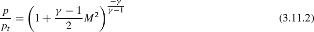
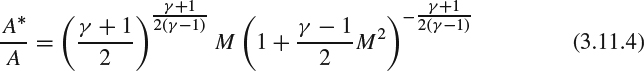
where A is the streamtube area, a is the speed of sound, and the star refers to conditions that would apply at Mach 1. These relations are plotted in Figure 3.11.2, and they highlight several very useful facts regarding steady inviscid flow of a perfect gas:

1. Streamtube area is at a minimum, and therefore mass flux per unit area is maximum, at a local Mach number of one. Thus for a flow to pass from a subsonic condition to supersonic, it must pass through Mach one at a local minimum in streamtube area. If geometric constraints force the flow area to go through a minimum at some location, as is the case in flows in confined passages or “ducts,” a maximum-mass-flux flow condition at Mach one at that location is often referred to as “choked.” To produce a steady supersonic flow in a duct, as in a rocket exhaust or a supersonic wind tunnel, a choked nozzle somewhere upstream is generally required.
2. A change in streamtube area has opposite effects in subsonic and supersonic flows. An area increase slows a subsonic flow down and increases the pressure and temperature but does the opposite to a supersonic flow.
3. Dimensionless ratios of flow quantities depend only on Mach number and γ. Changing the level of pressure or temperature has no effect on dimensionless ratios if Mach number is kept the same.

Steady, 1D flow analysis can be extended to include effects of bulk-averaged heating or cooling, or viscous friction. Treating such effects in a 1D, bulk-averaged sense can be a reasonable approximation for flows in ducts that are sufficiently slender relative to their length. The inclusion of these effects means that entropy and total pressure will no longer be constant. A flow with simple viscous friction and no heat transfer will still have constant total temperature, but a flow with heat transfer will not. Analytic solutions such as those leading to Equations 3.11.2–3.11.5 are possible for constant streamtube area and simple friction or simple heat transfer. Numerical solution is generally required in cases with variable streamtube area and/or combined effects. Equations applicable to these situations are derived in Shapiro (1953, Chapters 6–8)

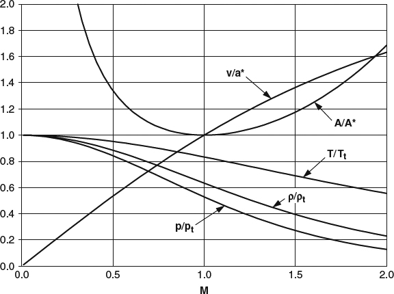
Figure 3.11.2 1 D isentropic-flow relations

3.11.2 Relations for Normal and Oblique Shock Waves

In solutions to the NS equations, compression shocks appear as continuous compressions in which all flow quantities vary smoothly. The predicted shock thickness of a bit over one mean free path is roughly correct, but the detailed distributions of flow quantities are not, because the NS equations don't model the molecular transport terms accurately when changes take place over such short distances. The “jumps” in flow quantities across a shock are accurately predicted because they don't depend on the internal structure of the shock, and the NS equations enforce all the relevant physical conservation laws that must be obeyed in the total jump across the shock.

Note that most practical numerical solutions to the NS equations are done on grids that are far too coarse to resolve the correct thickness of a shock. Numerical dissipation smears shocks over a distance of at least several grid intervals, which is typically several orders of magnitude larger than the actual thickness of a shock, and the degree of smearing increases when the shock front is oblique to the grid. Still, except to the extent that the smearing encroaches on flow gradients upstream and downstream, jumps across the shock can be predicted accurately in spite of the smearing.

The “shock relations” are a set of analytic formulas describing the effects of shocks in terms of the jumps in flow quantities from upstream to downstream. In this discussion, we will consider only steady flows, but the results of the steady theory can in principle be transformed to apply to unsteady flow because the flow in the neighborhood of a shock can be rendered locally steady by a Galilean transformation that cancels the motion of the shock normal to itself. The shock relations are “1D” in that they describe what happens only to an individual streamtube as it goes through the shock, and in this sense they are similar to the 1D isentropic flow relations we described in Section 3.11.1. The only multidimensional consideration that comes into play is turning of the streamtube through the shock, which must be accounted for when the shock is oblique to the local flow direction. Because jump conditions through a shock do not depend on the detailed internal structure of the shock, the shock relations can be derived in an essentially inviscid framework.

To derive the shock relations, we enforce conservation of mass, momentum, and energy across the shock discontinuity. Conservation of the component of momentum tangential to the shock requires that the jump in tangential velocity is zero. Because the tangential velocity is the same upstream and downstream, it can be removed by a Galilean transformation, and any shock can be viewed as a normal shock. The derivation is therefore carried out in two stages. First we derive the jump conditions for a normal shock, and then we derive the jump conditions for an oblique shock by transforming the normal-shock relations (i.e., by reversing the Galilean transformation that removed the tangential velocity).

For a normal shock, once we enforce conservation of mass, momentum, and energy; assume a perfect gas; and stipulate that entropy cannot decrease, the relationships between downstream and upstream flow quantities are uniquely defined. The resulting relations are plotted in the form of dimensionless ratios in Figure 3.11.3. A shock obeying these relations is often referred to a Rankine-Hugoniot shock (see Liepmann and Roshko, 1957). The following general characteristics of normal shocks are noteworthy:

1. The Mach number jump is always from supersonic to subsonic, with accompanying increases in pressure, temperature, and density, and a decrease in velocity.
2. Total temperature and total enthalpy are unchanged, but because passage through a shock is a dissipative process, there is a loss in total pressure and an increase in entropy. A jump from subsonic to supersonic (an “expansion shock”) would require a decrease in entropy and thus violate the second law of thermodynamics.
3. The “strength” of a shock, as indicated by the loss in total pressure, increases rapidly with upstream Mach number. In applications where low drag is important, really strong shocks are to be avoided by design, and the strength of relatively weak shocks becomes an important issue. An important fact to remember in that regard is that for upstream Mach numbers near 1.0 (the weak shock limit), the total-pressure loss goes as (M − 1)³.
4. Because of the loss of total pressure, the minimum area, A*, through which the flow can be forced, is increased by passage through the shock.
5. Dimensionless ratios between downstream and upstream are unique functions of either upstream or downstream Mach number and γ.

Of course, the normal-shock relations apply to oblique shocks as well, provided we resolve the velocity and Mach number in the direction normal to the shock. So the basic physics of an oblique shock is no more complicated than that of a normal shock. With oblique shocks, however, there is a surprising degree of apparent additional complexity, introduced by what amounts to only one additional free parameter in the problem (the tangential velocity). Across an oblique shock, the normal velocity is reduced, and the tangential velocity is unchanged, so that the flow is turned, or deflected, through some angle as it passes through the shock. For a given upstream Mach number, which must be supersonic, there is a maximum deflection angle. For any deflection angle less than the maximum, there are two possible shock inclination angles and two different possible downstream flow conditions. For deflection angles close to the maximum, both of the possible downstream conditions are subsonic, as would be the case with a normal shock, but for deflection angles less than the maximum by more than a fraction of a degree, one of the possible downstream conditions is supersonic. These complexities are best understood through study of the various oblique-shock charts in Shapiro (1953) or NACA Report 1135 (Ames Research Staff, 1953).

Figure 3.11.3 Normal-shock relations

The normal and oblique shock relations we've just discussed are essentially 1D, but they apply in multidimensional flows. When supersonic flow is present in steady-flow solutions of the multidimensional inviscid equations (the Euler equations), shocks are usually also present and appear as surfaces imbedded in the field, across which flow quantities are discontinuous. Flow quantities can also be discontinuous across imbedded vortex sheets, or singularities can exist at discontinuities in the slope or curvature of bounding surfaces, but everywhere else in the field flow quantities are continuous and differentiable, and the inviscid equations of motion are satisfied. The locations and shapes of imbedded shock surfaces are not known or specified a priori; all that can be specified is that if a shock arises as part of the solution, the jump across it must satisfy the shock relations. In mathematical jargon, solutions with such imbedded surfaces of discontinuity are called “weak” solutions. Note that the Euler equations, which are satisfied in the regions of continuous flow, are not sufficient to determine the solution if any shock discontinuity is present and that the shock relations must be imposed explicitly across the discontinuity. In numerical solutions, shock discontinuities can either be represented explicitly (shock fitting) or approximated automatically in a somewhat smeared-out way in the numerical grid (shock capturing). We'll discuss these options further in Section 10.4.1.