7

Lift and Airfoils in 2D at Subsonic Speeds

In a way, lift is the most visible of the aerodynamic forces. We see heavier-than-air animals and machines flying through the air every day, and something has to be holding them up there. Of course, we can predict the existence of aerodynamic lift mathematically by solving equations of motion for the flow around the lifting object. The accuracy of such predictions depends on the level of fidelity of the equations we choose to solve and varies with the type of lifting-surface shape and with the flow situation. Some types of lifting flow are easier to predict accurately than others. In principle, however, if we had the computing power available to carry out a direct numerical simulation (DNS) solution of the Navier-Stokes (NS) equations for the flow, we would be able to predict any lifting flow, 2D or 3D, with high accuracy. So in one sense, the physics of lift is perfectly understood: Lift happens because the flow obeys the NS equations with a no-slip condition on solid surfaces.

On the other hand, physical explanations of lift, without math, pose a more difficult problem. Practically everyone, the nontechnical person included, has heard at least one nonmathematical explanation of how an airfoil produces lift when air flows past it. Such explanations fall into several general categories, with many variations. Unfortunately, most of them are either incomplete or wrong in one way or another. And some give up at one point or another and resort to math. This situation is a consequence of the general difficulty of explaining things physically in fluid mechanics, a problem we've touched on several times in the preceding chapters.

In the real world, lifting flows are never precisely two dimensional, even when we try to make them so, as we do in so-called “2D” wind-tunnel testing. It seems like it should be possible to produce precisely 2D airfoil flow in a wind tunnel: Just mount a 2D airfoil model so that it spans the space between parallel tunnel sidewalls. But in reality 2D flow is practically impossible to achieve because of viscous effects on the tunnel sidewalls and in the junctions between the model and the sidewalls, and results of “2D” wind-tunnel testing are always questionable to some extent. On many flight vehicles, however, wings are of high enough aspect ratio that the local flow at stations over most of the span behaves at least qualitatively like the 2D ideal. Thus exploring the physics and doing some of our design work in the ideal 2D world makes sense. Even trying to simulate 2D flow in the wind tunnel can be useful in spite of the generally imperfect results. In this chapter, we'll concentrate on nominally 2D flow because it's simpler, and we can learn a lot that is generally applicable.

In this chapter, we'll start with the easy part: the mathematical prediction of lift through solutions of equations of motion, and the closely related (and still mathematical) explanations of lift in terms of circulation and vorticity. Then we'll look at physical explanations of lift in 2D, starting with a discussion of the strengths and weaknesses of many of the explanations already in circulation. With these cautionary tales in mind, we'll try to develop our own “best we can do” physical explanation of lift in 2D. Then we'll discuss some of the major physics and design aspects of airfoils. In Chapter 8, we'll extend the discussion from 2D to 3D.

7.1 Mathematical Prediction of Lift in 2D

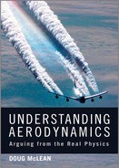
The earliest attempt that we know of to predict lift mathematically was Newton's theory for the lift of an inclined flat plate. Unfortunately, Newton got it wrong, but that is forgivable, given that his theory predates any rational theory of continuum fluid dynamics by more than a 100 years. Newton assumed a “bullet” model for the flow, as shown in Figure 7.1.1, in which particles do not interact with each other before they strike the forward-facing surface of the body, and no particle strikes the aft-facing surface, a model whose shortcomings we've already discussed in Section 5.1.

Assuming that the particles that strike the plate transfer the perpendicular component of their momentum to the plate and retain the parallel component, Newton predicted that lift is proportional to the square of the angle of attack, for small angles. The square relationship arises because the theory predicts that lift is proportional to both the number of particles intercepted per unit time and the momentum absorbed from each particle and that both increase with angle of attack. Later we'll see that in continuum lifting flows, we get a linear relationship (ideally) between lift and angle of attack, largely because the angle of attack has very little effect on the amount of fluid per unit time that the lifting surface effectively interacts with. So the square relationship is simply wrong, and for reasonable angles of attack, the magnitude of the lift predicted by Newton's model is much too small and was cited even into the late 1800s as a reason why heavier-than-air flying machines would never be possible.

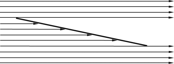
Figure 7.1.1 Newton's model for the lifting flow around an inclined flat plate (an application of the “bullet model” of Figure 5.1.1)

To get the right answer, we must model the continuum behavior of the fluid correctly. I've already claimed that a DNS solution of the full unsteady NS equations does this and should, in principle, predict any lifting flow with high accuracy. This claim is untested, however, because such a calculation has yet to be carried out for any Reynolds number typical of an aeronautical application. For routine calculations with current computers, we must scale our ambitions back to solutions of the Reynolds-averaged Navier-Stokes (RANS) equations with turbulence modeling (see Section 3.7). At this level of fidelity, we can predict lift with reasonable accuracy, provided that the airfoil or wing is nicely shaped, has a reasonably sharp trailing edge, and is at a low enough angle of attack that the flow stays attached to both surfaces at least to within a short distance of the trailing edge. Fortunately, most airfoils that are of practical interest meet these requirements, and the attached-flow regime covers much of the flight envelope of most flight vehicles, so that this predictive capability is highly useful.

As the angle of attack is increased, however, and boundary-layer separation moves forward on one surface, the accuracy of RANS predictions generally deteriorates, primarily because turbulence models are less accurate for separated flows than they are for attached boundary layers. As the angle of attack increases further, the separated region becomes larger yet, the real flow becomes increasingly unsteady, and most numerical schemes for the steady RANS equations will at some point fail to converge to a steady solution. Obtaining realistic solutions for flows with large separated-flow regions requires solving for at least the large-scale unsteady motions associated with the separation. It is not enough simply to solve the unsteady Reynolds-averaged Navier-Stokes (URANS) equations. The calculation procedure must somehow enforce a proper distinction between the large-scale motions that can be computed and the small-scale turbulence that must still be modeled. Large-eddy simulation (LES) and detached-eddy simulation (DES) are approaches that are under exploratory development, and we'll look further at them in Chapter 10, but they are not yet in routine use.

At the next step down in fidelity from steady RANS solutions with turbulence modeling, we find the various viscous-inviscid coupling schemes in which the flow is divided into an outer inviscid region and an inner boundary layer. With the right kinds of coupling and solution schemes, such methods can predict much of the same class of flows that can be predicted by RANS, including flows with small separated regions, and within the range where they can produce converged solutions, their accuracy can be comparable to that of RANS solutions. The widely used ISES and MSES codes (Drela and Giles, 1986; Drela, 1993) are examples of this class of methods. A disadvantage of coupled methods is that they tend not to handle geometric complexity as well as RANS, especially in 3D.

Even viscous-inviscid coupling solutions require extensive computation and have been practical only since the early 1970s. Before that, flowfield prediction for airfoils was restricted to inviscid flow. The loss of fidelity incurred by the neglect of viscous effects depends on the type of airfoil and the flow conditions. At low Reynolds numbers, boundary layers are thick and usually have major effects on the pressure distribution. In the transonic regime, the pressure distribution is extremely sensitive to the effective shape of the airfoil and is therefore sensitive to the displacement effect of the boundary layer. But for airfoils with sharp trailing edges in the attached-flow regime, at moderate-to-high Reynolds numbers, and outside the transonic regime, predictions of lift and pressure distributions from inviscid-flow theory can be adequate for many purposes. In Section 7.4.1, we'll look at this issue further, using computational examples to assess the magnitude of viscous effects on lift and pressure distributions in incompressible flow at moderately high Reynolds numbers.

The easiest way to obtain solutions for inviscid flow is through potential-flow theory, which for much of the twentieth century provided our only means for predicting the lift and pressure distributions of airfoils in 2D flow. As simple and powerful as potential-flow theory is, however, applying it to lifting flows gives rise to a couple of interesting mathematical difficulties. The first difficulty is in representing a lifting flow at all in terms of a velocity potential in the manner defined by V = ∇ ϕ (see Section 3.10 for an introductory discussion of potential-flow theory). Two requirements must be satisfied. First, if a potential function is to represent a continuous velocity field, the potential must be continuous and have continuous first derivatives. Second, the Kutta-Joukowski theorem, which we'll discuss in detail in Section 7.2, tells us that we must have circulation around the airfoil if we are to have lift. These requirements conflict: A single potential function that is continuous throughout the domain surrounding the airfoil cannot represent a flow that has nonzero circulation. This follows from the definition of the velocity as the gradient of the potential. The line integral of the velocity on a contour from any point A to any other point B must be equal to the change in the value of the potential between the two points. If there is nonzero circulation on a closed contour from point A back to point A, then the potential must have two different values at point A. Thus if we are to be able to represent flows with nonzero circulation, we must relax the requirement for continuity of the potential by defining a branch cut from some point on the surface of the airfoil to infinity, as shown in Figure 7.1.2, across which a jump in the value of the potential, but not the first derivatives, can take place. Note that the jump in potential across the cut is equal to the circulation around the airfoil and must therefore be the same everywhere along the cut. Note also that for any given velocity field with circulation, it doesn't matter where we put the branch cut. The only requirement is that there be a cut.

Even after we've introduced a branch cut to allow for flows with circulation, another difficulty remains. The potential jump across the branch cut is now a free parameter in the problem that our potential equation and boundary conditions are not sufficient to determine. A solution exists for any value of the potential jump and the circulation. Thus the lift, which is the main thing we seek to predict, is indeterminate. Figure 7.1.3 illustrates this problem, showing streamline patterns for the same airfoil shape with different values of circulation, all of which satisfy the potential equation and the boundary conditions. Kutta (Durand, 1967a) proposed a resolution to this indeterminacy, observing that the only physically reasonable solution is the one in which the flow leaves the trailing edge smoothly, as in Figure 7.1.3b. This criterion for choosing the preferred value of the circulation is known as the Kutta condition. Note that it resolves the non-uniqueness of the potential-flow solution only if the airfoil has a single sharp trailing edge.

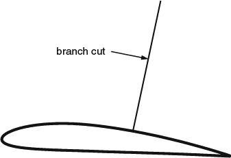
Figure 7.1.2 Illustration of a branch cut to allow a velocity potential to represent a flow with circulation around an airfoil

Figure 7.1.3 Sketches of potential-flow streamline patterns around the same airfoil shape with different values of circulation. (a) Zero circulation; zero lift. (b) Circulation such that flow leaves trailing edge smoothly; some lift. (c) More circulation; higher lift than (b)

Over the many years since Kutta introduced it, there has been much discussion of what the Kutta condition really means, physically speaking. Some critics have seen it as a mathematical artificiality and argued that the need for it demonstrates the physical inadequacy of potential-flow theory. The holders of this harsh view seem to be in a minority, however. The more prevalent view is that when a physical theory leaves out some physical effect, it is reasonable to adopt a rule or adjustment if it can be shown to effectively compensate for what was left out. In the case of potential-flow theory, what was left out is the combination of viscosity and the no-slip condition. It is often observed that viscous flow cannot generally negotiate a sharp corner, as in Figure 7.1.3a,c, without separating, and that the presence of viscosity is therefore the reason that the flow pattern of Figure 7.1.3b is the only physically reasonable one. In this view, the Kutta condition is seen as a perfectly reasonable proxy for one of the major effects of viscosity; that is, that viscous flows tend to separate from sharp edges.

The compensation that the Kutta condition provides is not perfect, but it is quite effective. It resolves the indeterminacy of the lift and enables potential-flow theory to predict something close to the right lift-versus-alpha curve and airfoil pressure distributions in the attached-flow regime, but it leaves the displacement effect of the boundary layer unaccounted for (see Section 4.1.3 for a discussion of the displacement effect in general, and Section 7.4.1 for examples of the effects of displacement on the lift curve and pressure distribution of an airfoil).

Of course, an “edge” doesn't have to be perfectly sharp to provoke viscous-flow separation, and in the real world separation will still anchor itself near the trailing “edge” of an airfoil even if there is a considerable degree of rounding. Thus even if the trailing edge is rounded, something like the Kutta condition still applies, albeit with some uncertainty as to where it applies.

So the Kutta condition is reasonably seen as accounting for the major effect of viscosity. A logical extension of this line of thinking is that lift would not exist without viscosity. It can be shown, based on starting the flow from rest, that in the absence of viscosity, the nonlifting flow pattern of Figure 7.1.3a is the one that would occur (see Gentry, 2006). There is some experimental support for this conclusion, though it is not extensive. Fluids without viscosity exist only in the form of superfluids such as liquid helium, and these have been produced in the laboratory only in small volumes in which the usual kinds of aerodynamics experiments can't be done. There has been one experiment in which a tiny propeller was suspended on a slender fiber in a flow of superfluid liquid helium (Donnelly, 1967). There was no detectable torsional deflection of the fiber, indicating that there was no lift on the propeller's blades. I don't know how definitive this result is. Given the small scale of the experiment, it's unlikely that the trailing edges were very sharp on the scale of the blade chord.

A possible alternative mechanism for the Kutta condition in gas flows is compressibility. Compressible flow around a sufficiently sharp trailing edge would expand to a vacuum condition, with no plausible way for the flow to reach the stagnation point on the other surface. Thus even in the absence of viscosity, we might still see the Kutta condition obeyed through the effects of compressibility, a possibility we consider in more detail in Section 9.1.5.

In the early years of our discipline, even solutions for incompressible potential flow around general airfoil shapes required too much computation to be practical. As we noted in Section 3.10, analytic conformal mapping provides a way to generate solutions for fairly “complicated” shapes with practically no computing. By applying this method, Joukowski (Durand, 1967a) was able to define some reasonably practical-looking airfoil shapes and predict their pressure distributions. Another simplification, developed by Munk around 1920 (Durand, 1967a), is the linearized inviscid theory, applicable in the limit of small thickness and angle of attack. We'll consider the linear theory further in Section 7.4.1, where we find that it provides interesting insights into the effects of shape and angle of attack on an airfoil's pressure distribution.

7.2 Lift in Terms of Circulation and Bound Vorticity

A major relationship that can be derived from momentum conservation and kinematic considerations (circulation and vorticity theorems) is that lift is always accompanied by circulation and vorticity. In Section 7.1, we saw how this relationship must be accounted for in potential-flow solutions for 2D airfoil flows. It is also a key ingredient in quantitative theories of lift and induced drag in 3D, as we'll see in Sections 8.2 and 8.3. And it plays a role in a particular kind of explanation of lift in general, as we'll see below, though not the kind of physical explanation we'll be seeking in Section 7.3.

The most basic statement of this relationship is the Kutta-Joukowski theorem (Joukowski, 1906). As originally derived, it applies to lift in 2D, but it also applies to stations along the span of a 3D wing in the limit of high aspect ratio. The theorem states that the lift per unit span on a 2D airfoil of any shape in a steady, inviscid, irrotational flow is proportional to the circulation Γ on a closed contour enclosing the airfoil:

where ρ and U_∞ are the density and velocity at infinity. The contour on which Γ is defined can be any closed contour enclosing the airfoil, because the flow everywhere outside the airfoil surface is assumed irrotational, and Stokes's theorem (Equation 3.3.4) then requires that Γ must have the same value regardless of what closed contour is chosen. In a real, viscous flow, the theorem should still apply with high accuracy, provided the contour is outside the boundary layer and doesn't cut the viscous wake too close to the trailing edge.

Now, given that lift requires circulation around the airfoil, Stokes's theorem also requires that any closed contour enclosing the airfoil must have a net spanwise vorticity flux passing through it, equal to the circulation. This vorticity is referred to as bound vorticity because it is associated with the airfoil itself and is not convected away from the airfoil by the flow. Consider four ways that the bound vorticity can be thought to reside with the airfoil, in decreasing order of realism:

1. In a real, viscous flow with a physical boundary layer on the surface of the airfoil, the bound vorticity is the actual physical vorticity in the boundary layer, as illustrated in Figure 7.2.1a. The bound vorticity is therefore distributed over some short distance off the surface into the flowfield. In a steady boundary-layer flow, vorticity is replaced by convection from upstream and diffusion from above or below as fast as it is convected away by the flow, so that it is as if the vorticity were stationary, and we can still think of it as bound vorticity (see Section 4.2.4 for a discussion of the vorticity “budget” of a boundary layer).
2. In an inviscid flowfield like we assumed in the derivation of Equation 7.2.1, the bound vorticity cannot reside anywhere in the interior of the field because the flow is irrotational. The vorticity must therefore reside on the airfoil surface, as shown in Figure 7.2.1b. It takes the form of an ideal vortex sheet, which is a sheet of zero thickness in which the vorticity is infinite, but the vorticity flux (strength) per unit width of sheet is finite, a concept we discussed in Section 3.3.7. The strength of the sheet is equal locally to the magnitude of the potential-flow velocity at the surface, which is consistent with having the interior of the airfoil filled with fluid at rest and with the idea that a vortex sheet defines a velocity jump, as we saw in Section 3.3.8.
3. In either of options (1) or (2) above, the vortex sheets on the upper and lower surfaces consist of vorticity of opposite signs, and their effects are partially offsetting. What really counts out in the field is the sum of the upper and lower surface contributions, or the net vorticity at each longitudinal station along the chord, which in some models of the flow is taken to reside in a vortex sheet on a camber line between the upper and lower surfaces, as illustrated in Figure 7.2.1c. This picture simplifies things considerably and is usually what is meant when the term “bound vorticity” is used. We'll find that thinking just of the net vorticity makes it easier to think about what happens in the flowfield around a 3D wing, which we'll take up in Section 8.1.2. The picture also applies naturally to an airfoil with zero thickness, in which case the vorticity strength is equal to the magnitude of the velocity difference (jump) between the upper- and lower-surface flows.
4. In some highly simplified models that are used when only the farfield effect is important, the bound vorticity is represented by a single vortex, usually placed at the quarter chord, as shown in Figure 7.2.1d.

Of course, the viscous wake downstream of the trailing edge in 2D flow also contains vorticity, but of opposite signs in the upper and lower portions of the wake. At any longitudinal station along the wake, the net vorticity (integrated over the thickness of the wake) is thus a difference between contributions of opposite sign. The near wake of a lifting airfoil usually has some curvature and therefore a pressure difference and a velocity jump across it, both usually small. This means that the net vorticity convected past the trailing edge is small but not exactly zero. As the wake straightens out downstream, the net vorticity in it must go to zero. For this to happen, any net vorticity that was there in the near field must be destroyed by viscous diffusion between the vorticity of opposite signs in the upper and lower portions of the wake. Then practically no net vorticity is convected out of the near field by the wake. The global situation is as if all the vorticity resided close to the surface (the bound vorticity), and there were no other vorticity in the field, just as it was for the inviscid-flow case.

The usual derivation of Equation 7.2.1 invokes momentum conservation applied to a control volume with its inner boundary at the airfoil surface and its outer boundary far enough away that the velocity field can be approximated by the combination of the uniform freestream and a single vortex of strength Γ located on or near the airfoil, representing the integrated bound vorticity on the airfoil surface. The original derivation assumed incompressible flow, but it is sufficient to assume subsonic flow and small disturbances in the farfield.

Figure 7.2.1 Illustrations of the bound vorticity associated with a lifting airfoil, represented in different ways, in order of decreasing physical fidelity. (a) As the vorticity in the physical boundary layer of a real viscous flow. (b) As an ideal vortex sheet on the surface itself, in an inviscid flow. (c) As the net vorticity of the upper and lower surfaces, located on a camber line between the surfaces. (d) As a single vortex at the quarter-chord location

So conservation of momentum in control-volume form, combined with Stokes' theorem, tells us that lift must be accompanied by circulation and bound vorticity. Note, however, that Equation 7.2.1 is just a relationship between the lift and the circulation, and that it doesn't predict what the lift or circulation will be for a particular airfoil shape and flow condition. To predict the lift, we must still solve for the flowfield to some level of fidelity, as discussed in Section 7.1. And, of course, Equation 7.2.1 doesn't explain what causes the circulation.

7.2.1 The Classical Argument for the Origin of the Bound Vorticity

An argument to explain the origin of the circulation and thus the existence of lift is given by Prandtl and Tietjens (1934) and by Batchelor (1967). It follows the airfoil through the process of a start from rest and relies more on observation of experimental flow visualizations and on circulation and vortex theorems than on direct physical reasoning. The argument can be paraphrased as follows:

Note that this scenario is more of a description of the process by which circulation is established than it is an explanation. To the extent that it is an explanation, it is more logical and mathematical than physical, as all the crucial steps along the way are justified by mathematically derived theorems: Kelvin, Helmholtz, and Kutta-Joukowski. The theorems are correctly applied, so the logical inferences are correct. But they do amount more to logical inferences than to physical explanations.

A further shortcoming of this argument as an explanation of lift in general is that it concentrates on a particular time sequence by which lift can be established (an impulsive start from rest at a fixed angle of attack) and “explains” only one aspect of the final steady state (the circulation). One might wrongly infer from the Prandtl-and-Tietjens scenario that the final steady-state lift depends on the details of the initial time history. But the final steady state is nearly always a unique “stable attractor” that is the end point of any one of an infinity of time histories (impulsive starts, gradual starts, varying angle of attack, etc.). Thus the final steady state is in a sense more fundamental than any of the possible starting sequences, and a more satisfying explanation would deal directly with it and show us why it does what it does. And this would require establishing more details than just the circulation.

The Prandtl-and-Tietjens scenario falls short of being a real physical explanation in other ways as well. First, it assumes the existence of the starting vortex and supports it only by appealing to experimental flow visualizations. Just how or why the vortex forms is never explained. Then it strays into questionable cause and effect when it says that “Owing to the formation of the starting vortex, the velocity field is changed … ” This implies that vorticity is somehow a cause of the velocities that occur elsewhere, which reflects an incorrect interpretation of the Biot-Savart law, as we saw in Section 3.3.9. Otherwise, the Prandtl-and-Tietjens scenario, as presented, neglects to assign any cause-and-effect relationships or at least fails to make a distinction between logical inference and physical cause.

The general order in which the argument is presented leads the reader to infer that lift is a result of the formation of the starting vortex. The overall logical inference is true, that if a starting vortex was shed, then there must be lift on the airfoil. But this particular inference works just as well in the opposite direction: If there is lift on the airfoil, then a starting vortex must have been shed. The general direction of physical cause and effect is such that it would be closer to the truth to say that the lift force is the prime mover, and the starting vortex is a result of it, not a cause.

Batchelor's version of the explanation also refers to experimental flow visualizations, but it dwells in greater detail on the initial phase of the formation of the starting vortex, and it makes a more convincing argument that the shedding of vorticity is a necessary consequence of viscosity. Overall, however, it also implies that the shedding of the starting vortex somehow causes the establishment of the circulation on the airfoil.

A close analogy to the relationship between lift and the starting vortex is the relationship between a bear walking through the woods after a fresh snowfall, and the paw prints he leaves behind in the snow. The presence of the prints allows the logical inference that a bear has passed by since the snowfall. But this works in the opposite direction as well: Knowing that a bear has passed through soft snow allows the equally logical inference that prints must have been left. The logical inference can work either way, but the physical cause-and-effect relationship is clearly one-way: The passage of the bear caused the prints, but the prints did not cause the passage of the bear. Like a paw print in the snow, the starting vortex is a mostly passive trace left behind by other physical events. It is not a cause of those events.

In “The Origins of Lift,” Gentry (2006) recounts essentially the same scenario as Prandtl and Tietjens, but he goes on to describe some key features of the airfoil flowfield, such as the upwash ahead of the airfoil, the higher velocity over the upper surface, and the downwash behind the airfoil, as being caused by the “circulatory flow.” Actually, these features are just parts of the circulatory flow pattern, and it isn't logical to say they are caused by it. Assigning causation to “circulatory flow” in this way is also closely related to the idea that vorticity at one location can “cause” velocities elsewhere, which is incorrect, as we saw in Section 3.3.9.

7.3 Physical Explanations of Lift in 2D

In this section, we seek to explain lift in 2D flows, in the context of continuum fluid mechanics, but without appealing to mathematics, both to further our own physical understanding and to have a satisfactory explanation that we can share with nonexperts. We've already alluded to what a difficult task this is, and because it is so difficult we'll end up devoting a lot of attention to it. Not only do we have to deal with the complexity of the physics, but we will also have to address an extensive collection of nontechnical lore that this topic has generated over the years, most of which is deeply flawed. Because of this, we'll end up spending more time on the background than on the explanation itself. But all this effort is justified by the general importance of the issue. An explanation for what causes lift is probably the single most important thing most laymen want to know about aerodynamics.

First, we'll look at some of the general characteristics of many of the explanations that are already in circulation (no pun intended) and discuss their strengths and weaknesses. With that as background, we'll set down our “requirements” for a more satisfying explanation, and then we'll proceed to compile our “best” explanation. We'll divide this into a basic part that can be shared with a nontechnical audience, followed by some additional technical details.

7.3.1 Past Explanations and their Strengths and Weaknesses

The purpose of this section is not to provide an exhaustive recounting of the explanations that have been offered in the past, but to look at some of the general lines of argument they share and to assess their strengths and weaknesses.

7.3.1.1 A General Observation on the Nature of the Problem

I propose that an underlying reason most of the explanations we'll discuss below fall short is that they set out to do more than is logically possible, given the nature of continuum fluid mechanics. In Section 3.5, we discussed how predicting what will happen in a fluid flow requires solving the equations of motion, something we can't generally do in our heads with sufficient precision to choose the “right” solution from the many kinematically possible flow patterns. Yet, in most of the proposed physical explanations of lift, there is an implied assumption that a simple linear argument starting from a few basic principles can both predict and explain the existence of lift and that no prior knowledge of the characteristics of the flowfield is required. We'll discuss this issue further when we set down our “desired attributes of a more satisfactory explanation” in Section 7.3.2.

7.3.1.2 The Flowfield-First Fallacy

A line of thinking that characterizes many of the physical explanations for lift that have been proposed is something I call the “flowfield-first” fallacy. It shows up most seriously in Bernoulli-based explanations, but it creeps into other explanations as well. The general line of argument is first to determine, by some argument or other, what the flow around the airfoil does and then to deduce that the flow exerts a lift force on the airfoil. There is no mention of whether the lift force influences what the flow does. It is not always explicit that the flow “causes” the force, but causation is implied by the way the inferences run. What is implied is one-way causation of the kind that I argued in Section 3.5 is incompatible with continuum fluid mechanics, in which cause-and-effect relationships tend to be reciprocal. Any argument that claims to establish what a flowfield does, without reference to the forces that it exchanges with its environment, must be at least incomplete. Note that the mathematical predictions of lift that we discussed in Section 7.1 don't share this failing because, in solving equations of motion for the continuum behavior of the fluid, they determine the flowfield and the force together, taking into account the proper circular cause-and-effect relationships.

So the flowfield-first approach is faulty at the outset, in assuming that we can determine key features of the flowfield that will lead to a lift force, and that we can make the determination without knowing that the lift force is there. The Bernoulli-based explanations are the most serious offenders in propagating this fallacy, but they tend to have other faults as well, as we'll see.

7.3.1.3 Bernoulli-Based Explanations

The key flow feature that Bernoulli-based explanations appeal to is a region of high velocity that forms over the upper surface of the airfoil, which is then said to imply, or even cause, low pressure on the upper surface, as a consequence of Bernoulli's principle. Causation is not always explicitly stated, but it is implied. We'll see later that lower pressure and higher velocity over the upper surface are indeed necessary for lift. But the implication that the high velocity causes the low pressure amounts to the same kind of one-way causation that we just saw in connection with the flowfield-first fallacy, applied now at another level of detail in the flowfield, and it is wrong for the same reason. Again, one-way causation is simply not compatible with the physics. In this case, the high velocity and the low pressure are indeed related, but it is wrong to explain the causation as running only in one direction. And this error effectively dooms any explanation built along these lines. Because the low pressure is seen only as a result of the high velocity, and not as part of the cause, it is impossible to explain correctly how the high velocity got there in the first place. Most attempts to explain the high velocity without appealing to the pressure follow either of two main approaches, both unsatisfactory.

7.3.1.4 Longer Path and Equal Transit Time

This is an argument that is widespread in explanations aimed at the layman. In this approach, it is assumed that the upper surface of the airfoil is more convex than the lower surface, which is often true but not always, and that the path the air must follow around the upper surface is therefore longer than the path around the lower surface. It is further assumed that fluid parcels that are split apart at the leading edge to traverse the upper and lower surfaces must rejoin at the trailing edge as shown in Figure 7.3.1. Thus fluid parcels negotiating both paths must do so in equal transit times, and we conclude that the velocity over the upper surface must be higher than that over the lower surface.

Figure 7.3.1 Fluid parcels splitting at the leading edge of an airfoil and rejoining at the trailing edge according to the erroneous equal-transit-time assumption

This explanation is wrong for several reasons that we'll address next, but first we should note that relative path length doesn't work well as an indicator of how much lift an airfoil can produce. First, lift can be produced with zero difference in path length. For an airfoil consisting only of a camber line (no thickness), there is an ideal angle of attack at which the flow attaches smoothly to the leading edge, and the upper- and lower-surface flows see the same path length. For example, a camber line consisting of a segment of a circular arc produces lift at its ideal angle of attack of 0°. Then, even among airfoils that do have a difference in path length, the difference tends to be no more than a small percentage. This is an order of magnitude too small for the path-length explanation to account for the lift that airfoils actually produce, as Craig (1997) has pointed out. Airfoils under real lifting conditions can produce much lower pressures and much higher velocities over the upper surface than any reasonable path-length difference can account for. So where does the path-length explanation go wrong?

First, the assumption of equal transit time is wrong. There is no reason why fluid parcels that split at the leading edge must rejoin at the trailing edge. But to say more about relative transit times, we need to observe one careful distinction regarding what fluid parcels we are going to follow to measure the transit time. In real viscous flows, we assume that the no-slip condition holds, with zero velocity at the solid surface, so that transit times for parcels passing close to the surface approach infinity. Even in ideal inviscid flows there is a similar problem. In practically all 2D airfoil flows, the initial attachment of the flow is at a stagnation point at which the velocity is zero and away from which the velocity initially increases linearly, and again, transit times for parcels passing close to the surface approach infinity. This is an example of the infinite delay effect for blunt-nosed obstacles in general that we discussed in connection with Figure 5.1.3c. To get around this difficulty, we must measure the transit time for parcels that start their journeys at some arbitrary distance above or below the stagnation streamline upstream, and in the case of viscous flow, the distance should be chosen large enough so that the parcels remain outside the boundary layers on the upper and lower surfaces. When we do this, we find that under lifting conditions, parcels that traverse the upper surface make the trip in less time and get to the trailing edge before the corresponding parcels that traverse the lower surface. Parcels that started close together near the attachment streamline ahead of the airfoil end up permanently displaced from each other after they pass the trailing edge, as shown in Figure 7.3.2.

Figure 7.3.2 Fluid parcels splitting at the leading edge of an airfoil and ending up displaced from each other downstream in an ideal lifting flow that satisfies the Kutta condition

The equal-transit-time explanation is problematic on another level as well, and that is that it is not a real physical explanation. Simply saying that something must go faster than something else to get somewhere at the same time does not explain how it goes faster, for example, by identifying the physical force that accelerates it to a higher velocity.

7.3.1.5 Hump, Half-Venturi, or Streamtube Pinching

As usually presented (see Anderson, 2008, Section 5.19, for example), this approach also assumes that the upper surface is more convex than the lower surface. The argument then assumes a general flow pattern along the lines of what we discussed in Section 5.1, what I called the “obstacle effect.” The upper surface acts as a kind of “hump” or larger obstacle to the flow than does the lower surface, with the result that the streamlines over the upper surface are pinched together more than those over the lower surface. Then, as a result of streamtube mass-flux conservation, the velocity is higher. As an alternative to the “hump,” an analogy is sometimes drawn between the upper surface of the airfoil and the inner surface of a Venturi tube, but this is essentially the same argument.

This explanation is better than the longer-path-length explanation in that the velocity difference that it might account for is not so limited. But as usually presented, it has two major flaws:

1. It doesn't really explain how streamtube pinching comes about at all, let alone why it is greater over the upper surface than over the lower surface. Streamtube pinching is not a kinematic necessity, as we saw in Section 5.1 in the discussion of Figure 5.1.4, so a dynamical explanation for it is needed. Anderson's (2008) version offers only that the flow somehow “senses the upper portion of the airfoil as an obstruction” and pinches down to go around it. I assume this is not meant to say that a fluid flow actually has some kind of remote-sensing capability, just that in pinching down the flow behaves as if it were sensing the presence of the airfoil. Still, this leaves unexplained what physical principle is at work in the pinching-down response. Really explaining streamtube pinching requires getting into the details of the dynamics, as we did in our discussion of the obstacle effect in Section 5.1.
2. Appealing to mass-flux conservation (continuity) isn't very satisfying as a physical explanation for higher velocity. Conservation of mass is a fundamental physical principle, but at the flowfield level it is really more of a kinematic constraint than a dynamical relation (see Section 3.4.1). Really understanding why something speeds up requires looking at the forces.

Some versions of this explanation argue that the airfoil needn't be more convex on the upper surface and that a positive angle of attack is sufficient to cause the leading edge to act as a hump and produce high velocity over the upper surface near the leading edge. The explanation by Eastlake (2002) is in this category. This version of the hump argument has some appeal in that it provides a basis for the variation of lift with angle of attack, but it still has the major fault of not providing a satisfactory explanation for how the streamtube pinching and the high velocity happen. We can also counter this argument with the observation that it doesn't rule out the zero-lift flow pattern of Figure 7.1.3a, in which the trailing edge also acts as a hump, producing high velocity on the lower surface near the trailing edge.

7.3.1.6 Confusion Regarding Low Pressures

Confused thinking about what low pressure actually means, physically speaking, seems to be widespread, and the confusion isn't limited to explanations of airfoil lift. We all tend to think intuitively of lower-than-ambient pressure as something that can exert a pull on surfaces that it touches. For example, Shevell (1989) uses a tornado as an example in his discussion of the low pressure in the core of a vortex, and states that “The low pressure is the force with which a tornado removes the roof from a house.” This of course can't be true in a literal mechanical sense. Even the lowest pressure reachable in the core of a tornado must still be positive in an absolute sense, and therefore cannot by itself be the force that lifts a roof. If a roof is lifted, it is lifted by the pressure beneath it. The low-pressure air above the roof plays its part by not pushing down as hard as it ordinarily would. The low pressure doesn't directly provide the force that lifts the roof.

The idea that low pressure can exert a pull finds its way into some airfoil explanations that discuss the low pressure on the upper surface. It is mostly explanations aimed at popular audiences that are guilty of this, and it is often seen in both the graphic illustrations and the words.

In the graphics accompanying many explanations, the pressure distribution around the airfoil surface is plotted as an array of vectors (arrows) normal to the surface. The trouble is that the vectors' magnitudes are made proportional to the local pressure difference, relative to ambient, so that high pressure is shown as arrows pointing toward the surface, and low pressure is shown as arrows pointing away from the surface, as seen in Figure 7.3.3a. One could argue that this convention is perfectly fine for conveying quantitative information and that it shouldn't cause confusion for a technically literate audience, provided the basis is explicitly spelled out. However, the quantitative data could be conveyed more easily and clearly in a conventional Cartesian plot. In representing the pressure as arrows with directions, the intent is clearly not just to convey data, but also to provide a physical feel for how the pressure acts as a force. In this regard, an illustration like Figure 7.3.3a is misleading, at least to a nontechnical reader, because it gives the impression that the air in regions of low pressure is pulling on the surface.

To provide the physical feel that Figure 7.3.3a seeks to provide, but to do it without misleading, is problematic. We could make the lengths of the arrows proportional to the absolute pressure, as in Figure 7.3.3b. In this case, we have had to assume the equivalent of a relatively high subsonic Mach number, so that the pressure differences are large enough to stand out relative to the magnitudes. And this is the only drawback to this type of presentation: It exaggerates pressure differences compared to what would actually occur, say, in a general-aviation application at low Mach numbers where the pressure differences would be too small to see clearly.

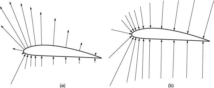
Figure 7.3.3 Airfoil pressure distributions represented graphically as vectors. (a) Arrows proportional to the pressure difference p − p_∞. (b) Arrows proportional to the absolute pressure

The words that accompany an illustration like Figure 7.3.3a are often as misleading as the illustration. The word “suction” is often used to refer to the pressures that are lower than ambient. As a technical usage, there is nothing wrong with this, as long as everyone understands that it just means “lower pressure than ambient.” But for a nontechnical reader, it is potentially confusing because it tends to evoke an image of the air pulling on the surface, like the arrows in Figure 7.3.3a.

Another idea that is often put forward is that the upper surface produces most of the lift, because the negative pressure differences on the upper surface, relative to ambient, are on average larger in magnitude than the positive pressure differences on the lower surface. Of course, if we look at it in terms of the actual physical forces, it is more correct to say that the air pushing against the lower surface is responsible for all of the lift, and then some, and that the air over the upper surface helps out by not pushing down as hard as the lower-surface air pushes up. But the view in terms of differences from ambient also has some merit. After all, the absolute ambient pressure would be there even if the airfoil were at rest, and it is the differences from ambient that result from the dynamics of the flow and are responsible for the lift. And it is true that the negative differences on the upper surface are generally larger than the positive differences on the lower surface.

It is often implied that this is a general characteristic of the production of lift, which is only partly true. According to the linearized theory we'll discuss in Section 7.4.1, lift results from the angle of attack and camber shape only, and airfoil thickness makes no contribution, to first order. For a cambered-plate airfoil (zero thickness) in the linear limit, lift is characterized by equal-and-opposite differences on the upper and lower surfaces. So for a very thin airfoil at a low lift level, the pressure differences associated with the lift are almost equal-and-opposite. But in most practical situations, both thickness and non-linear effects tend to reduce the pressure over most of the chord on both surfaces of the airfoil, so that the negative differences on the upper surface are actually larger than the positive differences on the lower surface.

7.3.1.7 Momentum-Based Explanations and the Coanda Effect

In momentum-based explanations, it is generally argued that the airfoil produces a flowfield in which some of the air is “deflected” downward and thus has downward momentum imparted to it. To acquire downward momentum, the air must have a downward force exerted on it by the airfoil, and thus, by Newton's third law, the airfoil must have an upward force exerted on it by the air. At the highest level, this general approach avoids the flowfield-first fallacy that mars most of the Bernoulli-based explanations. At least the mutuality of the force exchange between the airfoil and the air is explicitly acknowledged. But most explanations of this type fall short of providing a complete explanation of how the airfoil accomplishes the downward deflection of the stream.

Some momentum-based explanations emphasize that it is not just the lower surface of the airfoil that deflects the flow, and that the flow pattern over the upper surface also contributes strongly to the overall downward deflection. This general assertion is correct, but it is often followed by incorrect reasoning as to how the upper-surface flow does what it does. For example, Anderson and Eberhardt (2001) and Craig (1997) invoke the Coanda effect as the reason that the flow is able to follow the curved upper surface. This is problematic on more than one level:

1. Applying the term “Coanda effect” to an airfoil flow is inaccurate and therefore confusing. The Coanda effect usually refers to the tendency of a powered jet flow (in which the jet has higher total pressure than the surrounding fluid) to attach to an adjacent solid surface and to follow the contour of the surface. Although the attached boundary layer on the surface of an airfoil is a shear layer, it is not the same as a powered jet, and is not usually considered an example of the Coanda effect. As we'll see below, there is a limited way in which something like the Coanda effect can be construed as playing a role in airfoil flows, but it is a bit of a stretch.
2. The Coanda effect is erroneously seen as implying that viscosity plays a direct role in the ability of a flow to follow a curved surface. Anderson and Eberhardt assert that viscous forces in the boundary layer tend to make the flow turn toward the surface, specifically, as they put it, that the “differences in speed in adjacent layers cause shear forces, which cause the flow of the fluid to want to bend in the direction of the slower layer.” Actually, there is no basis in the physics for any direct relationship between shear forces and the tendency of the flow to follow a curved path.

First, we'll look at what the term “Coanda effect” properly encompasses, and then we'll consider what “flow attachment” or “boundary-layer attachment” in ordinary aerodynamic flows really involves and how it differs from the Coanda effect.

The phenomenon that Coanda himself investigated, for which others later coined the term “Coanda effect,” was limited to powered jet flows in which the jet is of the same phase (gas or liquid) as the surrounding fluid and has higher total pressure. A relatively thin 2D or annular jet (a jet in the form of a sheet) has a tendency to bend and attach itself to an adjacent solid surface, and to follow the surface even if the surface has strong convex streamwise curvature. This tendency is a result of the jet's entrainment of surrounding fluid and of the requirements imposed on the flow pattern by the continuity equation.

The effect is illustrated in Figure 7.3.4. In (a), we see an isolated 2D jet flowing into otherwise quiescent air. Whether the flow issuing from the nozzle is turbulent or not, at high Reynolds numbers the jet downstream will be turbulent, and the important thing for our purposes is that a turbulent jet strongly entrains fluid from the surroundings as it spreads downstream. Outside of the turbulent jet itself, the fluid flows toward the jet, thus feeding the entrainment. The velocities required to feed the entrainment are not large, but they are important, as we'll see. In (b), we've introduced a solid surface adjacent to the jet, with the leading edge of the surface close to the edge of the jet, but with the rest of the surface curving increasingly away from the jet. Because we've placed the surface in a region that in the case of the isolated jet was nearly quiescent air, we might naively expect it not to have much effect on the high-velocity flow in the jet, and for the jet to continue to flow straight, as it did in (a). But blockage of the flow feeding the entrainment makes it impossible for the flow pattern of (b) to be sustained. The air between the jet and the surface is entrained faster than it is replaced from the surroundings, and the flow quickly switches to the pattern in (c), where the jet bends to flow along the curved surface. The pressure field simultaneously adjusts (Remember circular cause and effect between velocity and pressure!) so that a pressure gradient normal to the local flow direction balances the centrifugal force associated with the curvature of the flow. So we see that even in a jet flow that exhibits the Coanda effect, the curvature of the flow is not a direct result of viscous forces (or their turbulent counterparts), but an indirect one.

In ordinary aerodynamic flows without powered jets, flow attachment has very little in common with the powered-jet effect that Coanda investigated and is really just the absence of boundary-layer separation. In Section 4.1.4, we saw that boundary-layer separation from a smooth surface in a 2D flow generally requires rising pressure (an adverse pressure gradient) to stagnate the low-velocity fluid. Counteracting the effect of an adverse pressure gradient is the favorable viscous force by which the higher velocity fluid farther from the surface drags the low-velocity fluid along. Boundary-layer separation thus involves a tug-of-war between the adverse pressure gradient and an opposing viscous force. At any given station along a surface subjected to an adverse pressure gradient, the pressure gradient will generally be winning the tug-of war locally, slowing the fluid near the wall, and reducing the velocity slope at the wall. How far the boundary layer perseveres into the adverse pressure gradient before it separates depends on the rate at which the pressure gradient wins and the velocity slope at the wall decreases. Until the slope of the velocity profile at the wall is brought to zero, the boundary layer remains attached, just like the corresponding inviscid flow would under the same conditions. Separation occurs only when the adverse pressure gradient has acted over a long enough distance to produce reversal of the velocity profile. Thus the role of viscous forces in maintaining boundary-layer attachment is to reduce the deceleration caused by the pressure gradient and to help the low-velocity fluid at the bottom of the boundary layer keep moving, and the viscous forces are needed only in situations where the pressure gradient is adverse. Viscous forces have nothing direct to do with causing the flow to turn and follow a curved surface.

Figure 7.3.4 Illustration of the Coanda effect. (a) Isolated free jet in otherwise quiescent air. (b) Curved surface added adjacent to the jet, but not altering the flow. (c) Jet attached to the curved surface

There are two things that very likely have contributed to confusion regarding this issue:

1. The boundary layer on the surface of the airfoil is effectively a sheet of vorticity. In Section 3.3.5, we saw that one of the kinematic properties of vorticity is that fluid parcels have a solid-body-rotation component to their motion, with angular velocity ω/2. If we picture an airfoil oriented so that the flow is from left to right, fluid parcels in the upper-surface boundary layer will have a solid-body-rotation component to their motion, in the clockwise direction. It seems intuitively natural that fluid parcels that are rotating will tend to follow curved paths (curved downward in this case). This is a pre-Newtonian sort of intuition, however, that has no basis in the physics (the meaning of “pre-Newtonian” is discussed at the end of Chapter 2). There is no connection between fluid-parcel rotation and curved paths in the flow.
2. There is an indirect association between surface curvature and the need for viscous effects in the maintenance of flow attachment. Convex surface curvature is often, though not always, associated with an adverse pressure gradient, in which case favorable viscous forces are needed to prevent separation. But the viscous forces prevent separation by dragging fluid along in the direction of the local flow, not by directly contributing to the turning of the flow.

If viscous forces make no direct contribution to the turning of the flow when the surface is curved, what actually causes the flow to turn? The answer to this question lies in the interplay between the velocity field and the pressure field, which works in the same way whether the fluid is viscous or not. When a flow turns to follow a curved surface, it is able to do so because the pressure field adjusts so as to provide the force needed to accelerate the fluid toward the center of curvature. Thus the centrifugal force generated when the flow follows a curved path is countered by a pressure gradient perpendicular, or normal, to the local flow direction. The normal pressure gradient and the flow curvature have a reciprocal relationship in which they cause and support each other simultaneously. This is just another aspect of the circular cause-and-effect relationship between the pressure and velocity fields that we discussed in Section 3.5 and that will figure heavily in the physical explanation for lift that we'll develop in Section 7.3.3. Note that the normal pressure gradient is perpendicular to the streamwise pressure gradient that we considered earlier and that it is the streamwise pressure gradient that plays the important role in determining whether the viscous boundary layer separates or remains attached.

So viscous forces play no direct role in ordinary flow attachment, contrary to Anderson and Eberhardt's explanation. A good counterexample to the Anderson and Eberhardt argument is the flow around a rotating circular cylinder with the freestream perpendicular to the cylinder axis. This is an example of a flow in which the tangential motion of the surface, due to rotation, affects the location of separation. In this case, the flow follows the curved surface farther around the side of the cylinder where the surface is moving with the flow, and it separates earlier from the side on which the surface is moving against the flow. But if we apply the Anderson and Eberhardt argument to this flow, it predicts the opposite of what is observed. On the side where the surface is moving with the flow, the viscous stresses are reduced or even reversed, and the ability of the flow to follow the curved surface would be reduced, according to their argument, but in fact it is enhanced. And vice versa for the other side of the cylinder. The observed effects on both sides are consistent with ordinary boundary-layer theory, which correctly accounts for the effects of pressure gradient and surface motion.

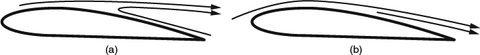
Figure 7.3.5 Candidate flow patterns around an airfoil at a moderate angle of attack. (a) Separation ahead of the trailing edge. (b) Attached flow to the trailing edge

We've looked in some detail at what the Coanda effect actually is, as it is usually understood to apply to a “powered” jet flow, and why it is not needed for ordinary flow attachment. But might there still be a way that it can properly be said to apply to airfoil flows? Perhaps, but it is at most a very limited way. Figure 7.3.5 shows two candidate flow patterns around an airfoil at a moderate angle of attack.

In Figure 7.3.5a, the flow separates ahead of the trailing edge and doesn't reattach to the surface, and in Figure 7.3.5b, the flow remains attached all the way to the trailing edge. At a low enough angle of attack, where the attached-flow pattern of (b) is the correct one, we could argue that what rules out the alternative separated-flow pattern of (a) is the same entrainment mechanism that is responsible for the Coanda effect. The separated shear layer of (a) entrains fluid faster than it can be replaced from downstream of the trailing edge. So for airfoils with attached flow to the trailing edge, we could say that it is something like the Coanda effect that rules out a separated-flow pattern. But this is not the same as saying that the Coanda effect is needed for the attached-flow pattern to be possible. The fact is that we needn't appeal to any viscous-flow mechanism, boundary layer, Coanda, or otherwise, to explain how flows can follow curved surfaces. Even ideal inviscid “flows” represented by solutions to the potential equation have no trouble following curved surfaces. And in real viscous flows, the natural tendency of the boundary layer is to remain attached unless it is provoked to separate by an adverse pressure gradient that is too strong, as we saw in Section 4.1.4.

7.3.1.8 The Water-Faucet Demonstration

In some explanations that refer to the Coanda effect (Anderson and Eberhardt, 2001, for example), a “simple experiment” is cited as a demonstration. If a curved object, like a spoon or a water glass, is held tangent to a small vertical stream of water from a faucet, the stream will deviate from its original vertical path and follow the curved surface, as shown in Figure 7.3.6a. This effect is obviously not a result of the same turbulent-jet entrainment that is responsible for the regular Coanda effect. Instead, it seems to be due to molecular attraction between the liquid and the solid and to the fact that the stream resists being torn apart, because of the surface tension at the water-air interface. These forces should be independent of the speed of the flow. Thus the amount of deflection they can produce should decrease as the speed of the stream increases, and, indeed, this seems to be the case. You can demonstrate to yourself that if the stream is sufficiently slow, the entire stream will follow the curvature of the glass, but if the stream is too fast, it will break up, and much of it will leave the surface of the glass without being deflected much, as shown in Figure 7.3.6b. In any case, such water-stream demonstrations are not relevant to explaining how aerodynamic flows follow convex surfaces.

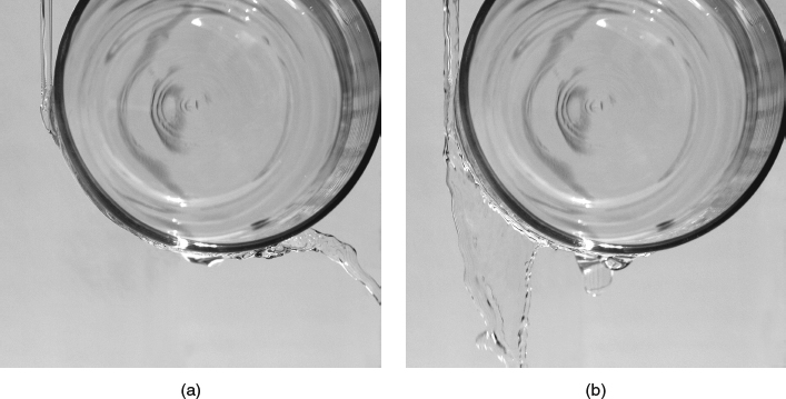
Figure 7.3.6 Water-faucet experiment that is sometimes proposed as a demonstration of the “Coanda effect” but actually demonstrates molecular attraction and surface tension (Photos by the author). (a) The slowest coherent stream that an ordinary garden nozzle can produce enters vertically downward on the left, adheres to the surface of a drinking glass, and is deflected through more than 90°. (b) A somewhat faster stream from same nozzle breaks up and is not deflected nearly as much

7.3.1.9 A Momentum-Based Argument in Which Flow Turning Comes First

A variation on the momentum-based argument is put forward by Weltner and Ingelman-Sundberg (2000) on their web site. It is noteworthy because it explicitly rejects the one-way causation from velocity to pressure that is common in Bernoulli-based explanations, but then implies one-way causation in the other direction. Their argument goes as follows (paraphrased):

This argument claims, in effect, that it is not correct to invoke a longitudinal acceleration (a change in speed) as the sole reason for a pressure change, but in the case of an airfoil flow, it is permissible to invoke the normal acceleration (a change in flow direction). The implied justification is that the primary effect of the airfoil surface is to force the flow to change direction and that it is therefore logical for the normal acceleration to precede the pressure change in the chain of cause and effect.

This idea has considerable intuitive appeal, but it is not entirely correct. The problem is that the interaction of most of the flow with the solid surface is not as direct as this argument implies. Only one vanishingly thin streamtube (the stagnation streamline) actually comes into contact with the airfoil surface, and the normal accelerations of all other streamtubes happen out in the field, just like the longitudinal accelerations do. For most fluid parcels, there is no direct interaction with the airfoil surface, only with adjacent parcels, and in this situation, there is no basis in the physics for making a distinction between the normal and longitudinal components of the acceleration. They are both just accelerations, and neither one has a one-way causal link to the pressure. The original argument correctly states that a change in flow speed requires a pressure difference. We can say the same thing about a change in flow direction: The only thing that can cause a change in the velocity vector is a pressure gradient. Thus for the normal acceleration to happen, the normal pressure gradient must already be there. And then if we incorrectly limit ourselves to one-way causation, we leave unanswered the question of what causes the pressure gradient. A correct explanation must acknowledge circular causation between the pressure and velocity fields.

7.3.1.10 The Bernoulli-versus-Momentum “Controversy”

Despite their flaws, both the Bernoulli approach and the momentum approach manage to get at parts of the truth. As we saw in Section 5.4, it is the pressure that transmits the lift force to any lifting body. And lift is invariably accompanied by low pressure on the upper surface and must therefore also be accompanied by elevated velocity outside the boundary layer, consistent with the Bernoulli explanation. Generating lift also requires deflecting the flow downward and imparting downward momentum, as in the momentum explanation. The Bernoulli and momentum explanations just appeal to different aspects of the same global phenomenon. The Bernoulli explanation is based on the near-surface flow and the surface pressure, while the momentum explanation is based on a manifestation of lift that extends into the far-field. They are not contradictory. However, having two different explanations that both seem “right” has led to some heated arguments, especially on some web sites that offer explanations of lift.

For example, there has been a tendency for advocates of either the Bernoulli approach or the momentum approach to argue that one is correct and the other is wrong, leading to a Bernoulli-versus-momentum (or Bernoulli-versus-Newton) “controversy,” as seen, for example, in much of the discussion accompanying the Wikipedia article on “Aerodynamic lift.” An alternative put forward by some other commentators is that both approaches are correct, but that they represent two separate mechanisms and two separate types of lift. The explanation on the ALSTAR instructional web site (Florida International University) is in this camp. According to this view, a flat plate at an angle of attack produces only “reaction lift,” and an airfoil with camber produces “Bernoulli lift” at zero angle of attack and adds “reaction lift” as angle of attack increases. The Bernoulli-versus-momentum controversy and the Bernoulli-lift/reaction-lift distinction are false, of course. Lift is a phenomenon that always involves a seamless combination of pressure difference and momentum transfer.

Another argument that is often made, as in several successive versions of the Wikipedia article “Aerodynamic Lift,” is that lift can always be explained either in terms of pressure or in terms of momentum and that the two explanations are somehow “equivalent.” This “either/or” approach also misses the mark. It's true that lift can be accounted for quantitatively either by the integrated pressure difference or by the momentum transfer. But such accounting doesn't constitute a satisfying physical explanation for how it all happens. A complete explanation must address all of the necessary aspects of the flowfield, and neither the Bernoulli nor the momentum approach is complete in this sense. As we'll see in Sections 7.3.3 and 7.3.4, a complete explanation must address both the velocity magnitude (Bernoulli) and direction (downward turning) because the flow we're trying to explain is not one-dimensional, but two-dimensional.

7.3.1.11 An Explanation Based on Flow Curvature

Babinsky (2003) begins by explaining the relationship between streamline curvature and the pressure gradient in the cross-stream (normal) direction, and he does so without any incorrect implication that the cause-and-effect relationship is one way. He then presents graphic illustrations of streamline patterns in flows around airfoils, showing that under lifting conditions the streamlines above and below the airfoil are generally curved downward. The pressure gradient (low pressure to high) is thus upward, and given that the pressure far above and below the airfoil must be close to ambient, the pressure on the airfoil upper surface must be low, and the pressure on the lower surface must be high, so that there is lift. Babinsky further shows that if the airfoil is thick, the high pressure on the lower surface may not materialize, but the pressure difference between the upper and lower surfaces can still provide lift. This explanation is correct as far as it goes, but it is incomplete in that it doesn't explain how the pressure gradients in the streamwise direction are sustained.

7.3.1.12 Lanchester's Explanation

An interesting early explanation was put forward by Lanchester (1907) and is paraphrased in the historical sketch by Giacomelli and Pistolesi, in Durand (1967). Lanchester first imagines a horizontal 2D flat plate (finite chord, infinite span) moving vertically downward, in effect a 2D planar parachute. There is, of course, a lift force on the plate, with low pressure above the plate and high pressure below, and air both above and below the plate is dragged downward. Because there can be “no permanent change of density or accumulation of matter in the lower strata of the atmosphere,” the downward current above and below the plate must be accompanied by upward currents around the edges of the plate, driven by the difference in pressure. This is the same general flow pattern that we discussed in Section 5.1 in connection with the “obstacle effect.” Lanchester imagined this motion to be associated with “a field of force established around the plane when the load was first applied: a field of force everywhere defined by the acceleration of the air particles.”

Lanchester then considers adding a horizontal motion to the vertical motion, so that the plate becomes a 2D “glider” descending along a sloped path. He deduces the resulting velocity field not by superposition of velocities, but by arguing that fluid particles passing through the same “field of force” that was there in the case of pure vertical motion

Note that although the velocity field with only vertical motion was symmetrical fore and aft, with upwash off both the leading and trailing edges, the field in the presence of forward motion is asymmetric, with downwash behind the trailing edge rather than upwash. Lanchester deduced from this flowfield picture that a slightly cambered airfoil, with the trailing edge turned down to enhance the downwash and the leading turned down to meet the oncoming upwash, should be superior to an airfoil with zero camber. Lanchester concludes that the vertical velocity of the air particles far ahead of and far behind the airfoil is zero, by the same argument as before, that a nonzero velocity would result in an accumulation of matter. He also concludes that there is no “continual transmission of energy to the air” and that the drag associated with such a 2D lifting motion is zero, ignoring skin friction.

Lanchester's explanation is intriguing for several reasons. The first is that it was developed so early in the history of the field, before the Kutta-Joukowski theorem was known and before potential-flow solutions for flows around airfoils had been derived. Further, and to its credit, Lanchester's explanation acknowledges a mutual relationship, rather than one-way cause and effect, between the velocity and the pressure (the “field of force”), and it provides an essentially correct account of some key features of 2D lifting flow: upwash ahead of the airfoil, and downwash behind, decaying to zero in the farfield. It does not explicitly address how lift varies with angle of attack, but it could easily be extended to do that. One weakness is that the 2D-parachute flowfield is not a very good model for the flow in the presence of forward motion. Of course, a steady parachute-type flow, with a massive separated wake above the plate, would be a terrible model. Lanchester avoided the problem of a separated wake by stipulating that we take the “field of force” to be that which existed at the moment when the load was first applied (the pressure field immediately after an impulsive start). Even so, this leads to a pressure field that is wrong in one important detail: The pressure field for a flat plate in vertical motion alone is symmetrical fore and aft, while the pressure field associated with forward motion at an angle of attack has a marked fore-and-aft asymmetry, as we'll see later. So Lanchester's explanation avoids some of the shortcomings of the other explanations that we've seen, but his flow model is inaccurate in some details.

7.3.1.13 An Unusual Argument for Downward Turning in the Nearfield

Hoffren (2001) argues that the streamline coming off the trailing edge of an airfoil at an angle of attack is directed downward and asymptotically levels off at a level below that of the trailing edge. Then, using essentially the same “no accumulation” argument that Lanchester (1907) used, he argues that the stagnation streamline approaching the leading edge must have started at the same low level. This means that the flow generally rises ahead of the airfoil and descends behind it and must therefore experience downward turning in the neighborhood of the airfoil. This kind of argument establishes that if the flow leaves the airfoil at a downward angle, there is a kinematic necessity for downward turning. But it doesn't establish a physical mechanism for the downward turning.

7.3.1.14 Two Other Recent Explanations

Craig (1997), in Stop Abusing Bernoulli – How Airplanes Really Fly, a book that has been popular in the airplane home-builder community, proposes an interesting wrinkle on the conventional momentum-based explanation, but unfortunately ends up generating more confusion than enlightenment. He draws attention to the upwash ahead of the leading edge of an airfoil and outboard of the wingtips of a finite wing, invoking the same reason for it that Lanchester did, that is, that to avoid an accumulation of matter, the downwash above and below the lifting surface must be accompanied by upwash elsewhere. For this upwash, he coins the term “recirculation,” apparently to reflect the idea that the air involved in the upwash motion was previously part of the downwash. But this idea correctly reflects the actual flowfield only far downstream of a wing of finite span, where the flow actually circulates around each member of a pair of trailing vortices. (We'll discuss the trailing vortex wake of a finite wing in some detail in Section 8.1.2.)

While the air immediately around the airfoil is part of a flow with circulation, as we saw in Section 7.2, none of it remains in the vicinity of the airfoil long enough to “recirculate” in any reasonable sense of the word, so the terminology is confusing at best. Furthering the confusion, Craig's Figure 2.5 shows a perspective view of a wing with arrows indicating that air from below the lower surface circulates forward, then upward in front of the leading edge, and then back, ending up above the upper surface. This picture might be correct if we isolated the circulatory part of the velocity field and regarded the arrows as streamlines of that part of the field, but Craig doesn't stipulate that that is what his Figure 2.5 represents.

If we interpret the arrows as particle paths, the picture is simply wrong. (Ordinarily in steady flows, particle paths and streamlines coincide, but not in this case, because the circulatory streamlines were constructed based on only a part of the velocity field.) In any case, the fact is that the air involved in the upwash ahead of the leading edge (and directly outboard of the tips of a finite wing) has not yet been involved in any of the downwash. Nevertheless, Craig refers to the upwash ahead of the airfoil as “recirculation” and assigns to it a major role in the production of lift. The accompanying discussion of transfers of kinetic energy from downwash to upwash and of lift being a “regenerative” process is confusing, and it is difficult to assess its physical correctness or lack of it.

A very clear description of the flowfield around an airfoil is given in See How It Flies, a web site for pilots, produced by a physicist (Denker, 1996). Many of the details of the flowfield and the pressure field around an airfoil are described and illustrated through excellent diagrams and animations. Cause-and-effect relationships at the local level, such as the relationship between pressure differences and flow curvature, and pressure differences and flow speed are described. At the global level, circulation and the Kutta-Joukowski theorem are discussed. Denker's presentation provides the reader with a wealth of information and physical interpretation, all to a high technical standard. Its only shortcoming, to my mind, is that it doesn't quite manage to show how all the pieces fit together, or to establish a complete web of cause-and-effect relationships at the global level.

7.3.2 Desired Attributes of a More Satisfactory Explanation

Every explanation we've looked at so far has been flawed in one way or another. We would of course like our explanation to avoid such flaws. But beyond that, what other attributes would we like it to have? Remember that we seek a physical explanation that does not require mathematics. In this regard, observing that we can predict lift by solving the NS equations is not a satisfactory explanation. Some, for example, Shevell (1989), have concluded that circulation and the Kutta-Joukowski theorem provide the only satisfactory explanation, but this is really just math as well. Besides, even if we were to accept the Kutta-Joukowski theorem as part of our explanation, it would just shift our problem from that of explaining where the lift comes from to that of explaining where the circulation comes from.

We acknowledge at the outset that it is not possible, without math, to predict the existence of lift, without knowing a priori some things about the flow that produces it. Providing ironclad “proof” that lift must exist is too much to expect, because that would require quantitative precision that is not available without computation or at least a simplified quantitative theory. Our objective is therefore to explain, not to predict or prove. Even though we've thus limited our objective, we still want our explanation to be as complete as possible, consistent with the correct physics. By “complete,” we mean the following:

1. Though it is fair game to assume a priori some knowledge of what the flow does, we should explain in a satisfying way how the flow does it.
2. Our explanation should be based on a logical application of physical principles and leave no gaps.
3. Not only should the logical inferences be correct, but the direct physical cause-and-effect relationships should be made clear.
4. The explanation should make clear not just how lift is produced, but also how the magnitude of the lift can be “controlled,” that is, how it varies with angle of attack and airspeed.

Although we have strong justification for relying on prior knowledge of what the flow does, we still tend to think of it as “cheating” somehow. We therefore have an inclination to try to define the minimum prior knowledge that needs to be assumed, and to try to deduce everything else from first principles. There is a strong appeal to the idea of an explanation that is maximally “self-sufficient” in this sense. But would such self-sufficiency really serve a pedagogical purpose? I think not. It seems to me that it would be better to assume the level of prior knowledge that makes for the clearest explanation, and that there is no disadvantage in assuming more than the minimum, provided it is all explained in the end.

So completeness and clarity are high on our list of objectives. There are also some faults we want to avoid:

1. Misrepresenting the phenomenon as being simpler than it really is. Given the subtlety of the phenomenon we're trying the explain, oversimplification is a great temptation, and it is a key weakness in many of the explanations we discussed in the previous section. Von Karman is reported to have said that in explaining things to a nontechnical audience, a Plausible Falsehood is preferable to the Difficult Truth (see Sears, 1994). I don't share this pessimistic view.
2. One-way causation of the kind we know is inconsistent with the physics, for example, “Lift is due to circulation” or “The pressure difference is caused by a velocity difference.”
3. Assuming something that isn't subsequently explained, for example, “Circulation means there is lift,” but not explaining where the circulation comes from.
4. Dependence on things that we know are not needed, for example, a sharp trailing edge or a curved upper surface.
5. “Naming” as a substitute for explaining, as, for example, in saying that a jet flow follows a curved surface because of the Coanda effect, where “Coanda effect” is just a name for the tendency of jet flows to follow curved surfaces.

An explanation that meets these requirements is not going to seem as tidy as most of the explanations we discussed in the previous section. However, as much as we'd like our explanation to be short and simple, we should resist the temptation to oversimplify and should aim for a level of detail and fidelity that does justice to the physics and meets our “completeness” requirement. A satisfactory explanation must resolve the Bernoulli-versus-momentum “controversy” and show how both pressure differences and momentum transfer are necessary parts of the picture. And it must blend these two seemingly independent aspects of the phenomenon into a coherent whole.

Ease of sharing favors an explanation that can be conveyed in relatively simple words, with no more graphic aid than can easily be sketched on a napkin. A drawback to simple graphics, however, is that the levels of detail and physical fidelity are limited. One way to increase the level of detail and to ensure fidelity is to introduce graphics with real quantitative accuracy. Going further in this direction, digital animation could probably be used to provide a level of “feel” for the physics that would be difficult to get any other way, for example, by illustrating time histories of forces and velocities as fluid parcels move through the field. But either of these high-tech options would reduce “portability.” My choice here is to try to achieve a satisfactory basic explanation without leaving the “talking/ sketching” realm.

Because our intent is to share our basic explanation with a “public” that will not have read the background in this book, and because we'd like our explanation to have some staying power, it behooves us to give some thought to its “fitness for survival” in the marketplace of ideas. Practically everyone we share our explanation with will have heard other explanations before ours and will hear more in the future. Superior correctness on the part of our explanation can help, but is not likely to be sufficient, because the general public receives little real-world feedback regarding the correctness of its understanding of aerodynamics. Dawkins (1976) drew an analogy between the survival of ideas in a human population and the survival of genes in a biological gene pool, and proposed that Darwin's insights on natural selection apply in both universes. He coined the word meme to represent units or groups of ideas that can be passed from brain to brain and whose survival depends on their ability to “reproduce” (spread) and on their resistance to being displaced by other ideas. The survival fitness of our explanation as a meme will be greatly enhanced if, in addition to providing superior correctness, it inoculates its hosts (the audience) against the errors they are likely to encounter in other explanations. To do that, our explanation should discuss some of the most common errors and explicitly call attention to what is needed to avoid them.

The basic explanation that follows is intended to stand alone and therefore repeats in simplified form some of the background in other parts of the book and some of the critiques of other explanations in Section 7.3.1. It comes as close to achieving the desired attributes stated above as I have been able to manage. It is longer than other explanations, but I have not found any way to shorten it significantly without compromising either completeness or correctness.

7.3.3 A Basic Explanation of Lift on an Airfoil, Accessible to a Nontechnical Audience

When a relatively thin, flat lifting surface such as a wing, a sailboat sail, or a shark's fin moves through air or water, it can produce a force perpendicular to its direction of motion. This force is called lift, whether or not it is in an upward direction.

Mathematical theories of lift have been agreed on by the experts since the early twentieth century, but there has been a long history of disagreement on how to explain lift in simple physical terms, without math. Over the last 100 years or so, many different nonmathematical explanations have appeared in books, popular magazines, pilot-training materials, museum exhibits, and so forth. These explanations follow a variety of approaches, but they generally try to make lift simpler than it really is, explaining too little about the flow and leaving important parts of the phenomenon unexplained. We'll consider the common examples below under “How the main popular explanations are incomplete.” And some explanations resort to erroneous arguments to explain features of the flow. These are discussed below under “Popular misconceptions.” Naturally the existence of numerous different explanations has been a source of confusion and controversy.

The following is a nonmathematical explanation of lift that attempts to resolve the controversies and to be scientifically complete and correct. It is necessarily more complicated and longer than earlier popular explanations.

7.3.3.1 Airfoil Shape and Angle of Attack

The cross-sectional shape of a lifting surface, as illustrated in Figure 7.3.7, is called an airfoil. How much lift a lifting surface produces depends on the shape of the airfoil, on the angle of attack at which it approaches the oncoming flow, and on flow speed and density. A positive angle of attack means that the leading edge (front) of the airfoil is positioned higher than the trailing edge (back), relative to the direction of the oncoming flow, as in Figure 7.3.7.

Almost any shape, as long as it is not too thick, will work as an airfoil and produce some lift when the angle of attack is in the right range. The main types of airfoil shapes are shown in Figure 7.3.8. A simple flat plate shape (a) is used on many toy gliders. The Wright brothers used a curved-plate airfoil shape (b) for the wings of their early airplanes because they found that adding curvature, or camber, increased lift. A toy glider will also fly much better with a curved-plate airfoil than with a flat-plate airfoil. Sailboat sails also generally take on the curved-plate form. Finally, larger model airplanes and full-size airplanes use streamlined airfoil shapes that are rounded at the leading edge and sharp at the trailing edge, (c) and (d). Aerobatic airplanes often use the symmetrical type (c), which works equally well right-side-up or inverted, while most other airplanes use streamlined airfoils with camber (d). Streamlined airfoils, especially those with camber, can produce more lift with less drag than other shapes, and they enable an airplane to fly over a wider range of speeds. Birds' wings tend to have a combination of the curved-plate and streamlined shapes (e).

Figure 7.3.7 The cross-sectional shape of a wing is called an airfoil, and the angle at which oncoming air approaches it is called the angle of attack

Figure 7.3.8 Types of airfoil shapes. (a) Flat plate. (b) Curved (cambered) plate. (c) Symmetrical streamlined shape. (d) Cambered streamlined shape. (e) Bird's wing

7.3.3.2 The Airfoil Reference Frame

The phenomenon of lift generation is the same regardless of what reference frame we view it from. We could watch the airfoil move through the air, but everything is easier to understand if we imagine ourselves moving along with the airfoil, so that the airfoil appears to us to be standing still and the fluid appears to flow past. And for simplicity we'll refer to the “upper” and “lower” surfaces of the airfoil assuming that the wing is positioned horizontally and is lifting upward.

7.3.3.3 Lift Involves Action and Reaction (Newton's Third Law)

An intuitive way to imagine that lift is possible is to think of the airfoil shape and angle of attack as working together so that the airfoil pushes downward on the fluid as it flows past. The fluid must then push back with an equal and opposite (upward) force, which is the lift. This is an example of Newton's third law, that every action has an equal and opposite reaction. Thus lift is an interaction in which the airfoil and the fluid exchange equal and opposite forces. The aspects of the interaction that need to be explained further have to do with how the moving fluid actually pushes back.

7.3.3.4 Lift Is Felt as a Pressure Difference on the Airfoil Surfaces

A fluid always exerts pressure, which just means that it always pushes against itself and against any surface that it touches. When the fluid around an airfoil is at rest, the pressure is practically the same everywhere, so that it pushes upward on the lower surface and downward on the upper surface equally, and there is no lift. When the fluid is moving and there is lift, the fluid exerts the lift force directly on the airfoil's surfaces as a difference in pressure: higher pressure on the lower surface than on the upper surface. Under lifting conditions, the average pressure on the lower surface is usually higher than ambient unless the airfoil is very thick, and the average pressure on the upper surface is always lower than ambient.

How large is this pressure difference, typically? In the atmosphere at sea level, the ambient pressure is about 2100 pounds per square foot. Compared with this, it doesn't take much of a pressure difference to provide a practical amount of lift. Even the heaviest airplane requires no more than about 150 pounds of lift per square foot of wing area. So the pressure difference that an airfoil must produce to support any airplane is much less than the “background” atmospheric pressure, and even when a wing is lifting, the pressure on the upper surface pushes down almost as hard, in absolute terms, as the pressure on the lower surface pushes up. The difference is what counts, and even a relatively small pressure difference, spread over a large enough area, can lift a 747.

7.3.3.5 Lift Involves Force and Acceleration (Newton's Second Law)

Explaining how the flow maintains the pressure difference described above requires looking at the forces exerted on the air and the resulting accelerations of the air, not just at the surface of the airfoil, but in an extended region around the airfoil. In the explanation below, we first identify the major features of the flow that are essential to maintaining the pressure difference, and then we consider how the whole combination satisfies Newton's second law.

The outline of the explanation is as follows:

• The fluid flows as if it were a continuous material that deforms to follow the contours of the airfoil.
• The airfoil affects the direction and speed of the flow within a deep swath above and below the airfoil in what is called a velocity field. Flow above and below the airfoil is deflected downward. Flow above the airfoil always speeds up, and flow below usually slows down.
• The airfoil affects the pressure over a wide area in what is called a pressure field. When lift is produced, a diffuse cloud of low pressure always forms above the airfoil, and a diffuse cloud of high pressure usually forms below. Where these clouds touch the airfoil they constitute the pressure difference that exerts the lift on the airfoil.
• The velocity field and the pressure field support each other in a reciprocal cause-and-effect relationship, an interaction in accordance with Newton's second law of motion.

Let's look at each part in more detail.

7.3.3.6 The Fluid Flows as if It were a Continuous Material that Deforms to Follow the Contours of the Airfoil

Fluids such as air and water consist of huge numbers of individual molecules that move randomly in all directions, even when the fluid appears to be at rest. In water, molecules are in constant contact with their neighbors as they move. In air, they are not in constant contact, but they collide frequently and travel only very short distances between collisions. If the molecules didn't have this random motion and never interacted with each other, they would fly directly into the forward-facing parts of the airfoil and not touch the aft-facing parts, as in Figure 7.3.9. Instead, because of the random motion and the frequent contact between molecules, the fluid flows as if it were a continuous material. It deforms and changes course to flow around the airfoil, and it fills all of the space around the airfoil and touches all of its surfaces, as illustrated in Figure 7.3.10.

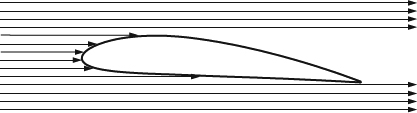
Figure 7.3.9 If molecules had no random motion and never interacted with each other, they would fly directly into the forward-facing parts of the airfoil and not touch the aft-facing parts

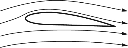
Figure 7.3.10 Because of the random motion and many collisions among its molecules, a fluid actually flows like a continuous material, deforming and changing course to flow around the airfoil, in what is called a flowfield

7.3.3.7 The Airfoil Affects the Direction and Speed of the Flow within a Deep Swath above and below the Airfoil in What Is Called a Velocity Field. Flow above and below the Airfoil Is Deflected Downward. Flow above the Airfoil Always Speeds Up and Flow below Usually Slows Down

Because the fluid deforms continuously as it flows, changes in direction are gradual, and the speed and direction of the flow vary over a wide area around the airfoil. A spread-out pattern of variations like this is often referred to as a flowfield or velocity field.

The airfoil's solid surface forces the flow very close to it to follow the direction of the airfoil contour, with the result that the speed and direction of the flow are affected over a wide area. And the flow is thus affected by both the airfoil shape and angle of attack.

When an airfoil produces lift, it deflects the fluid flow downward, as indicated by the streamlines sloping downward to the right in Figure 7.3.10 and by the downward-turning arrows in Figure 7.3.11. To produce the downward turning, the aft portion of the airfoil surfaces must have a predominantly downward slope. Thus to produce lift, the airfoil must have either camber or a positive angle of attack, or a combination of the two.

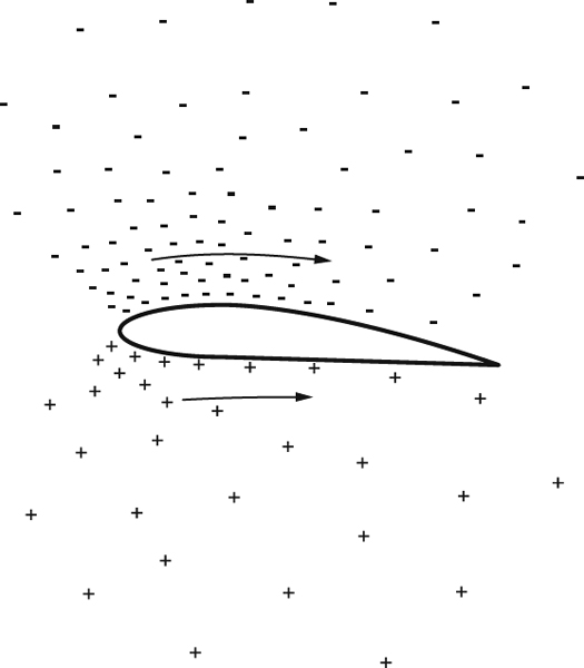
Figure 7.3.11 Illustration of the pressure field and the velocity field around a lifting airfoil. Minus signs indicate pressure lower than ambient, and plus signs indicate pressure higher than ambient. The tighter the spacing of the symbols, the larger the pressure difference

It seems obvious that downward-sloping airfoil contours should force the flow very close to the surface to be deflected downward, but it is important to understand that it is not just the flow close to the surface that is affected, and that the downward turning is spread over a deep swath of flow above and below the airfoil. The amount of downward turning is greatest close to the airfoil and dies away gradually far above and below.

In addition to the downward turning, the flow above the upper surface is always speeded up, as indicated by the longer arrow above the airfoil in Figure 7.3.11, and the flow below the airfoil is usually slowed down, as indicated by the shorter arrow. Like the downward turning described above, this effect is also strongest close to the airfoil surfaces and dies away gradually far above and below.

7.3.3.8 The Airfoil Affects the Pressure over a Wide Area in What Is Called a Pressure Field. When Lift Is Produced, a Diffuse Cloud of Low Pressure Always Forms above the Airfoil, and a Diffuse Cloud of High Pressure Usually Forms below. Where These Clouds Touch the Airfoil They Constitute the Pressure Difference That Exerts the Lift on the Airfoil

Because the fluid moves as if it were a continuous material, the airfoil influences much more fluid than its surfaces touch, producing pressure changes over a wide area. When an airfoil produces lift, there is always a diffuse cloud of low pressure above the airfoil, and there is usually a diffuse cloud of high pressure below, as illustrated by the clouds of minus signs and plus signs in Figure 7.3.11. Note that the minus signs don't mean that the pressure is negative, just that it is lower than ambient. These pressure differences are generally largest at the airfoil surface, where they actually exert the lift force, and away from the airfoil they die away gradually in all directions: above, below, ahead, and behind. A spread-out pattern of pressure differences like this is often called a pressure field.

7.3.3.9 The Velocity Field and the Pressure Field Sustain Each Other in a Reciprocal Cause-and-Effect Relationship, an Interaction in Accordance with Newton's Second Law of Motion

The downward turning of the flow, the changes in flow speed, and the clouds of low and high pressure described above are all necessary for the production of lift. They support each other in a reciprocal cause-and-effect relationship, and none would exist without the others. The pressure differences exert the lift force on the airfoil, while the downward turning of the flow and the changes in flow speed sustain the pressure differences.

Although the clouds of low and high pressure depicted in Figure 7.3.11 don't have sharply defined boundaries, they are still effectively “confined” to a limited area, both vertically and horizontally. “Sustaining” the pressure differences essentially means maintaining this spatial “confinement” in both the vertical and horizontal directions. Neither direction can be said to be more important than the other. Both are essential.

To understand how this “confinement” of the pressure differences works, we start by imagining the flow to be divided into tiny “parcels” of fluid passing through the region around the airfoil. The interaction these parcels are involved in reflects Newton's second law of motion, a general relationship among mass, force, and motion. Every parcel is subject to Newton's second law because the fluid in the parcel has mass, and because the parcel's neighbors can exert a net force on it, through differences in pressure. When the pressure is higher on one side of a parcel than on the other, the forces pushing the parcel in opposite directions are not balanced, and there is a net force pushing the parcel in the direction from higher pressure to lower pressure. Examples of this are illustrated in Figure 7.3.12.

Net forces on fluid parcels can also come from internal friction due to the viscosity of the fluid. However, when the flow around an airfoil follows both surfaces all the way to the trailing edge, as it usually does, viscosity has only a small effect on the overall flow pattern, and for purposes of understanding lift, we need only consider the forces due to pressure differences.

Newton's second law tells us that when a pressure difference imposes a net force on a fluid parcel, it must cause a change in the speed or direction (or both) of the parcel's motion. But in fluid flows, this cause-and-effect relationship not a one-way street. The pressure difference causes a change in the parcel's motion, but the existence of the pressure difference depends on the parcel's motion. The relationship is thus mutual, or reciprocal: A fluid parcel changes speed or direction in response to a pressure difference, and its resistance to changing speed or direction (its inertia, due to its mass) sustains the pressure difference. The pressure difference can exist only if something is there to “push back,” and what pushes back is the inertia of the fluid, which is why the mass of the fluid is so important.

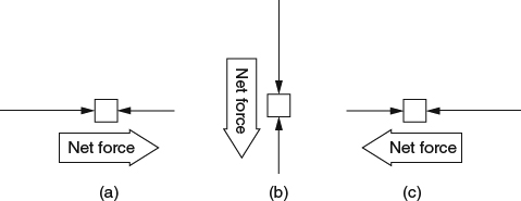
Figure 7.3.12 Examples of how pressure differences exert net forces on fluid parcels. higher on left: Net force to the right. (b) Pressure higher above: Net force downward. higher on right: Net force to the left

To show how this applies in the airfoil flowfield, Figure 7.3.13 illustrates how typical fluid parcels are acted upon by the pressure in different parts of the field. In different parts of the high- and low-pressure clouds, the pressure is increasing or decreasing in different directions, exerting forces on the fluid parcels as shown by the arrows.

Fluid parcels directly above and below the airfoil see higher pressure above them than below and thus see a net force that is mostly downward. The downward force is resisted by the downward acceleration, or downward turning, of the flow. This interaction between pressure and downward turning is reciprocal: The pressure difference acting on a fluid parcel causes the parcel's path to be deflected downward, and the pressure difference is sustained because the fluid parcel has mass and therefore resists having its path deflected from a straight line.

On the upper left, where flow is entering the region of low pressure above the airfoil, the net force on a parcel is from left to right, which is resisted by an acceleration in the direction of the flow, or an increase in flow speed. On the upper right, where flow is leaving the region of low pressure, it sees a pressure difference in the opposite direction and is slowed down. Thus a parcel passing through the cloud of low pressure above the airfoil is speeded up and then slowed back down. On the other hand, a parcel passing through the cloud of high pressure below the airfoil experiences the opposite sequence: It is slowed down and then speeded back up.

These changes in flow speed follow the relationship that is often referred to as Bernoulli's principle, which can be expressed mathematically as Bernoulli's equation. Bernoulli's principle applies to regions of steady flow that have not been affected significantly by viscous friction. There is a small part of the airfoil flowfield in which Bernoulli's principle doesn't apply, and that is in the thin viscous boundary layer next to the airfoil surface and a thin viscous wake downstream, where the flow is strongly affected by viscosity and is usually turbulent. However, the pressure field is largely determined in the larger part of the flowfield in which viscous effects are small, outside of the boundary layer and wake. There, Bernoulli's principle applies, according to which low pressure means high speed, and high pressure means low speed. This relationship is reciprocal: The differences in pressure in the horizontal direction cause the changes in flow speed, and the fluid's resistance to acceleration, because of its mass, sustains the pressure differences.

Figure 7.3.13 Pressure differences exert net forces on fluid parcels in different parts of the flowfield as indicated by the block arrows, and these forces are balanced by accelerations of the fluid parcels in the same directions

To summarize these interactions: The downward turning of the flow provides the vertical “confinement” of the clouds of low and high pressure, and the changes in flow speed provide the horizontal “confinement.”

Thus downward deflection of the flow and different flow speeds above and below the airfoil are both essential parts of the reciprocal cause-and-effect relationship that sustains (or “confines”) the pressure differences. The pressure differences cause the flow to change speed and direction, and the changes in flow speed and direction cause the pressure differences to be sustained. This circular cause-and-effect might seem a bit like “something for nothing” or “perpetual motion,” but it's not. The pressure differences follow naturally from the Newton's second law and from the fact that the flow close to the surface is forced to follow the predominantly downward-sloping contours of the airfoil. And of course the fact that the fluid has mass is crucial to the interaction.

In a way, it is surprising that mass is so important, given that air feels so light to our senses. However, air actually has more mass (and thus weight) than our intuition gives it credit for. In air at sea level, a volume of only about 14 cubic feet (a cube 2.4 ft on a side) weighs a pound. Thus even a modest volume of air contains significant mass, and an object moving through the air can influence a large mass of air in a short time. For example, the wing of a small airplane (a two-seat Cessna) flying at 100 mph causes significant changes in speed and direction in thousands of pounds of air every second.

7.3.3.10 The Roles of Camber, a Sharp Trailing Edge, and a Rounded Leading Edge

The downward-turning action that an airfoil produces is affected by both the airfoil shape and the angle of attack. The airfoil surfaces themselves need not be curved, and even the flat-plate shape of Figure 7.3.8a can produce downward turning when it has an angle of attack. However, adding camber to the airfoil shape, as in Figure 7.3.8b,d, aligns the airfoil surfaces better with the desired curved flow and enhances the downward-turning action. As a result, cambered shapes in which the upper surface is more convex than the lower surface produce more lift at a given angle of attack than shapes without camber.

What happens in the flow near the trailing edge plays an important role in controlling the downward-turning action. Figures 7.3.14 and 7.3.15 illustrate streamline patterns for low-to-medium angles of attack. Note that in both of these cases the flow from both the upper and lower surfaces leaves the airfoil smoothly from the trailing edge. If it didn't do this, the flow from one side would have to go around the trailing edge to the other side, as in Figure 7.1.3a. But viscosity generally prevents flow from going around a sharp edge in this way. So, with some help from viscosity, the trailing edge has the effect of directing the flow as it leaves the airfoil to flow in the direction of the contours of the aft part of the airfoil. This tendency of the trailing edge to direct the flow is a major reason why angle of attack and camber are so effective in influencing lift.

Figure 7.3.14 Streamline pattern at a low angle of attack: flow attaches near leading edge and follows the upper surface

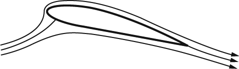
Figure 7.3.15 Streamline pattern at a medium angle of attack: flow attaches below the leading edge, flows around the leading edge, and follows the upper surface

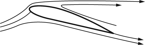
Figure 7.3.16 Flow around an airfoil at a high angle of attack breaks away from the upper surface, and the airfoil is said to be stalled

The situation at the leading edge is very different. Referring again to Figures 7.3.14 and 7.3.15, note that the flow around the leading edge changes dramatically when the angle of attack is increased. At a low angle of attack (Figure 7.3.14) the flow approaches the leading edge almost head on, while at a higher (medium) angle of attack (Figure 7.3.15) it approaches the leading edge from below and flows around the leading edge from the lower surface to the upper surface. In fact, the reason for having a rounded leading edge is to accommodate the different flow patterns at different angles of attack with a minimum of disruption.

7.3.3.11 How Lift is Controlled

Lift depends on the speed of the flow. An increase in speed increases the lift by increasing both the amount of fluid that the airfoil influences in a given time and the downward acceleration imparted to each bit of fluid. These two effects multiply each other, so that lift is approximately proportional to the square of the speed, at a given angle of attack.

Lift can also be increased by an increase in either the camber or the angle of attack, as long as the flow follows both surfaces of the airfoil, as it usually does at low-to-moderate angles of attack, as shown in Figures 7.3.14 and 7.3.15. For a given airfoil shape, this increase in lift continues until an angle of attack is reached above which the effects of viscosity prevent the flow from following the upper surface. The flow then breaks away, as shown in Figure 7.3.16, which is called stalling. As an airfoil passes through the stalling angle of attack, the lift generally decreases dramatically, though it doesn't disappear altogether.

Controlling lift through angle of attack is an essential ingredient in achieving controlled flight over a range of speeds. For steady level flight, the total lift on an airplane must be kept equal to the weight. When an airplane speeds up, it reduces its angle of attack in order to keep the lift from exceeding its weight. When an airplane slows down, it increases its angle of attack in order to keep the lift equal to the weight, but this works only up to the stalling angle of attack. Thus an airplane can slow down only so much, to what is called the stall speed, which is the minimum speed at which an airplane can fly steadily.

Lift also depends on the density of the fluid. A decrease in density decreases lift at a given angle of attack and speed by decreasing the mass of the fluid the airfoil acts on. Thus when an airplane flies at high altitude where air density is lower, it must either fly faster or increase its angle of attack in order to maintain lift equal to the airplane's weight.

Figure 7.3.17 A control surface deflected upward to decrease lift

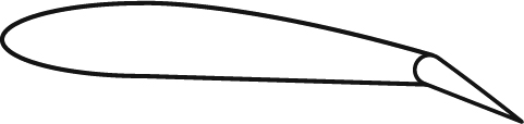
Figure 7.3.18 A control surface deflected downward to increase lift

Figure 7.3.19 A flap deflected downward to increase lift, with a slot to allow air to flow from the lower surface to the upper surface

Lift can also be controlled by what is called a control surface, which is just an aft portion of an airfoil that is hinged so that it can be deflected up and down, as shown in Figures 7.3.17 and 7.3.18. Deflecting a control surface changes both the effective angle of attack and the camber of the airfoil and thereby changes the flow-turning action. Examples of control surfaces are the elevators on the horizontal tail, which can pitch an airplane nose up or nose down, the ailerons near the wing tips, which can roll an airplane to one side or the other, and the rudder on the vertical tail, which can yaw an airplane in one direction or the other.

A flap is similar to a control surface and is deflected downward at the trailing edge of a wing to increase both the lift at a given angle of attack and the maximum lift that can be generated without stalling. Flaps enable an airplane to take off and land at lower speeds than it could without flaps. A flap often has one or more slots that direct air from the lower surface to flow over the aft upper surface, as shown in Figure 7.3.19, which helps to delay stalling.

Leading-edge devices such as leading-edge flaps or slats, as shown in Figure 7.3.20, also help increase maximum lift and allow slower takeoff and landing speeds.

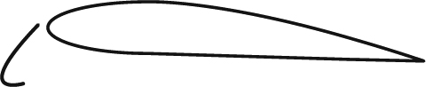
Figure 7.3.20 A leading-edge slat deflected downward to increase maximum lift

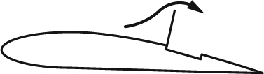
Figure 7.3.21 A spoiler deflected upward to disrupt the upper surface flow, decreasing lift and increasing drag

Spoilers are devices that hinge upward from the upper surface of a wing, as shown in Figure 7.3.21, disrupting the upper-surface flow by deflecting it upward, and causing a large decrease in lift and an increase in drag. When spoilers are used in flight, the purpose is not to decrease lift, but to increase drag and allow the airplane to descend steeply without speeding up. When spoilers are use in this way, the decrease in lift caused by the spoilers is compensated by an increase in angle of attack. When spoilers are used on the ground during the landing roll, the purpose is both to increase drag and to decrease the lift on the wing, putting more of the airplane's weight on the wheels to allow harder braking without skidding.

7.3.3.12 How the Main Popular Explanations Are Incomplete

The two most widely circulated explanations of lift are the momentum based (Newtonian) and the Bernoulli based. Both contain elements of the truth, but neither provides a complete explanation.

The momentum-based explanation generally goes as follows: When an airfoil produces lift, it deflects the flow downward, as indicated by the streamlines sloping downward to the right in Figure 7.3.10. Newton's second law tells us that to deflect the flow downward, the airfoil must push downward on the fluid. Then Newton's third law tells us that for every action there is an equal-and-opposite reaction, and the fluid must therefore push upward on the airfoil, and thus there is lift. This explanation is correct as far as it goes, but is incomplete in several ways. First, it doesn't point out that the force is actually transmitted to the airfoil by the pressure, and it doesn't explain how the airfoil can impart downward turning to a much deeper swath of the flow than it actually touches. Then although it hints at explaining how the pressure differences in the vertical direction are sustained, it doesn't explain at all how the pressure differences in the horizontal direction are sustained. That is, it leaves out the Bernoulli part of the interaction.

A Bernoulli-based explanation starts by arguing that the flow over the upper surface is speeded up, either because the path length over the upper surface is longer, or because of an “obstacle,” “hump,” or “Venturi” effect. Because of the higher speed, the pressure over the upper surface must be lower, according to Bernoulli's principle, and thus there is lift. Explanations of this type are incomplete in that they don't adequately or correctly explain what causes the flow to speed up. The longer-path-length explanation is simply wrong (see below, under “Popular misconceptions”). The “obstacle,” “hump,” or “Venturi” explanations are better, but only a little. They often mention “pinching” or “necking down” of the flow over the upper surface, but they don't provide a convincing physical explanation for the pinching. A common fault in all of these explanations is that they imply that a speed difference can arise from causes other than a pressure difference, and that the speed difference then causes, or at least implies, a pressure difference, according to Bernoulli's principle. This implied one-way causation is a misconception that we'll discuss below. Finally, a Bernoulli-only explanation doesn't really explain how the pressure differences in the vertical direction are sustained. That is, it leaves out the downward-turning part of the interaction.

There have been at least three schools of thought among proponents of the momentum-based and Bernoulli-based explanations. One is that only one or the other can be correct. Another is that both are correct, and that they apply to two different kinds of lift. A third is that both are correct, and either one suffices to explain lift in general. These are all misconceptions that we'll discuss next.

A third major category of explanation involves circulation around the airfoil. An explanation of this type starts with the observation that when an airfoil starts its motion through the fluid, a starting vortex is left behind. The formation of the starting vortex is accompanied by the establishment of a “circulatory flow,” or circulation, around the airfoil, which is responsible for the lift according to an aerodynamic theory known as the Kutta-Joukowski theorem. This is not a proper physical explanation for two reasons. First, it depends on several advanced mathematical and aerodynamic theorems instead of direct physical arguments. Second, although the argument is mathematically and logically correct, its general progression does not reflect physical cause and effect, and is therefore misleading. It implies that lift is somehow caused by the formation of the starting vortex and the resulting circulation. The starting vortex and the circulation are actually more properly seen as byproducts of the lift than as causes.

7.3.3.13 Popular Misconceptions

We've seen that lift generation involves subtle cause-and-effect relationships, so it shouldn't be surprising that many of the attempts to explain it to a popular audience have made errors of one kind or another. To solidify our understanding and make it less likely we'll be taken in by incorrect ideas, let's identify some of the misconceptions and consider where they went wrong.

This implication that the causation runs in only one direction is not consistent with the physics of fluid flows. If you try to explain a speed difference without referring to the pressure difference, you'll inevitably get the reasons for the speed difference wrong. One example of this, an erroneous reason for high velocity over the upper surface of an airfoil, is the next item on our list.

First, this isn't a proper kind of physical explanation. Just saying that something has to arrive somewhere at a particular time doesn't explain why the thing might speed up. To explain why something speeds up, we must identify and explain the force that makes it speed up. And this explanation is wrong on another level. There is no reason why fluid parcels that start together ahead of the airfoil must rejoin at the trailing edge, and in fact, they generally don't. A parcel that traverses the airfoil near the upper surface typically arrives at the trailing edge well ahead of one that traverses near the lower surface. So no difference in path length is required, and there are many situations in which lift is produced without a difference. And on airfoils where there is a difference, it is typically much too small to explain the speed difference that actually occurs when lift is produced.

We've seen that a pressure difference between the upper and lower surfaces and downward turning of the flow are both essential parts of the picture.

There is only one kind of lift, and explaining it requires both a pressure difference and downward turning.

Again, we've seen that a complete explanation must include both the pressure difference and the downward turning of the flow.

This reflects a misunderstanding of the role of viscosity in fluid flows and of what the Coanda effect actually entails. As fluid flows over the surface of an airfoil, there is no direct coupling between viscosity and flow turning, and none is needed. Viscosity plays a significant role in lift generation only in the immediate vicinity of the airfoil trailing edge, by preventing the flow from going around the trailing edge from the lower surface to the upper surface. The real Coanda effect refers to the tendency of a turbulent jet flow with higher energy than the surrounding fluid to attach itself to an adjacent surface and to follow the surface even if it is curved. This is not so much a viscous effect as it is an indirect effect of the jet turbulence. It arises because of the tendency of jet flows to entrain surrounding fluid, and it plays no role in ordinary airfoil flows.

Pressure, especially in gasses such as air, is always a push, never a pull. The pressure on the upper surface of an airfoil pushes downward on the airfoil, but the higher pressure on the lower surface pushes upward harder, and the net effect is lift.

The angle of attack is a key factor that determines how much lift an airfoil produces at a given flow speed and is an essential ingredient in achieving controlled flight.

7.3.3.14 Why There Have Been So Many Misconceptions

Explaining lift in physical terms is more difficult than most people realize, and the difficulty is inherent in the basic nature of fluid mechanics. We are dealing with countless little parcels of fluid that move in coordination with their neighbors and exert forces on their neighbors, all while separately and simultaneously obeying Newton's second law. It simply isn't possible to look at an airfoil and deduce, by mental effort alone, what flow pattern satisfies the physical laws everywhere at once. There are too many simultaneous relationships to keep track of. And the difficulty is compounded by the circular nature of the cause-and-effect relationship between pressure and velocity.

This kind of complexity isn't easy to deal with mathematically, either. Mathematically expressing all the relationships a fluid flow must satisfy results in a set of partial-differential equations called the Navier-Stokes equations. By solving these equations we can predict in detail what the flow around an airfoil does and how much lift is produced. But solving the equations means mathematically determining how the pressure and the flow velocity vary throughout a large volume of space surrounding the airfoil. For any given flow situation it requires lengthy calculations that are practical only on a high-speed computer. Computer programs are available that can make such calculations routinely. However, all they do is provide a simulation of what would happen in a real flow; they don't provide a physical explanation of how it happens.

Simplified theories have also been developed, such as potential-flow theory, which ignores viscosity, and the Kutta-Joukowski theorem, which relates lift to a circulatory component of flow (circulation) around the airfoil, but these don't provide a direct physical explanation for lift either.

So we see that predicting the existence of lift using nothing but the properties of the fluid and the laws of physics would essentially require solving the NS equations or the potential-flow equation for the flow around the airfoil, which is not something we can do in our heads. Explaining what happens, with words and simple diagrams instead of laborious calculations, thus requires some prior knowledge of what the flow does. The explanation above started with knowledge of some basic features of the pressure and velocity fields around an airfoil, and then showed how the pressure field and the velocity field support each other in a manner consistent with the laws of physics, including the proper reciprocal cause-and-effect relationships.

Faulty explanations often assume too little prior knowledge and then try to do more than is logically possible by mental effort alone. As a result, they tend to leave important things unexplained (such as what really causes the high velocity over the upper surface) and to resort to logical fallacies such as one-way causation.

7.3.4 More Physical Details on Lift in 2D, for the Technically Inclined

The above explanation of the interaction between the pressure field and the velocity field explicitly distinguished between vertical and horizontal confinement of the pressure differences. Readers with technical backgrounds will recognize this as one way of explaining to a lay audience an interaction involving a vector equation. In this case, the equation is the Euler momentum equation in 2D. Of course this equation has two components, both of which must be satisfied, and thus the necessity to explain two components of the interaction.

Above, in trying to explain why there have been so many misconceptions, we claimed that predicting lift strictly from first principles can't be done just through mental effort, that it requires laborious computation. To avoid going into too much detail for a lay audience, we deliberately neglected to mention that simplified theories such as conformal mapping or linear theory can greatly reduce the required computational effort. This is a justified omission because the simplified theories are still heavily mathematical, and they provide no aid to physical understanding by a nontechnical audience. But we will make use of the linear theory to further our own understanding of airfoil pressure distributions in Section 7.4.1.

The main thrust of our basic explanation was that lift is transmitted to the airfoil by a pressure difference between the upper and lower surfaces and that it requires at the same time a downward turning of the air stream above and below the airfoil. We ignored the upward turning, both ahead of the airfoil and behind, that accompanies lift in general and can be seen in Figure 7.1.3b. Referring again to Figure 7.3.11, note that the flow approaching the front of the airfoil sees higher pressure below it than above, and thus must receive a net push upward. It therefore turns upward, as indicated by the upward-curving streamlines ahead of the airfoil in Figure 7.1.3b. Then comes the downward turning above and below the airfoil that we've already discussed and connected with the generation of lift. Finally, the air behind the airfoil feels lower pressure above than below, and is turned upward again, as shown by the curving streamlines behind the airfoil, but only enough to cancel the downward direction it acquired as it passed the airfoil.

The flow angle actually approaches zero far from the airfoil, behind the airfoil as well as ahead. Does this mean that the downward turning that we associate with the lift has been canceled by the upward turning? Well, yes, but only in terms of the local flow direction. The net momentum change imparted to the air by the airfoil is still downward and still accounts for the lift.

To explain how this can be, we start with the fact that lift requires circulation, according to the Kutta-Joukowski theorem. An airfoil flow with circulation effectively consists of a uniform flow with disturbances associated with a collection of bound vorticity superimposed on it. In the simplest way of deriving the Kutta-Joukowski theorem, we define a control volume as shown in Figure 7.3.22, with vertical outer boundaries at the front and back, extending to infinity vertically. Conservation of momentum requires that the lift on the airfoil be balanced by the forces and momentum fluxes at these outer boundaries. Because the boundaries are vertical, there is no net vertical force contribution by the pressure, and the lift must be accounted for by the net flux of vertical momentum into the control volume. It can be shown that as long as the two faces of the control volume enclose all of the bound vorticity, the flux of upward momentum into the front face and the flux of downward momentum out of the back face account for half the lift each, regardless of the distances from the airfoil to the faces. And from this, we also arrive at a simple derivation of the Kutta-Joukowski theorem, Equation 7.2.1.

So the flux of vertical momentum through either face of the control volume of Figure 7.3.22 remains the same, regardless of how far away from the airfoil the face is placed. This is true in spite of the fact that the vertical velocity goes to zero at large distances. As either face is moved farther from the airfoil, the maximum vertical velocity decreases, but the distribution becomes more spread out vertically. This is illustrated in Figure 7.3.23 by plots of the downwash velocity -v on vertical cuts at different distances upstream and downstream of the airfoil. Upstream of the airfoil, the curves are to the left of their respective axes, which, given that we are plotting -v, indicates upwash. Downstream of the airfoil, the curves are to the right of their axes, indicating downwash. With increasing distance from the airfoil either upstream or downstream, the vertical velocity in the middle of the distribution decreases, while the vertical velocity in the “tails” of the distribution, above and below the level of the airfoil, increases, and the integrated flux of vertical momentum remains the same.

Figure 7.3.22 In the simplest derivation of the Kutta-Joukowski theorem, the farfield flow around an airfoil is modeled as a potential vortex superimposed on a uniform flow, and a control volume with vertical faces is used to assess the momentum flux due to lift

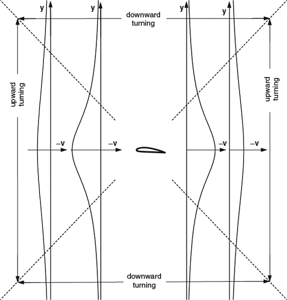
Figure 7.3.23 An illustration of the distributions of vertical velocity on vertical cuts at different distances ahead of an airfoil and behind. The vertical velocity is plotted as -v, so that in the upwash ahead of the airfoil the curves appear to the left of their respective axes, and in the downwash behind the airfoil, the curves appear to the right of their axes. The 45° dashed lines indicate the approximate dividing lines between upward turning and downward turning outside of the nearfield

Now it is clear how it can be that the upward turning of the flow (the reduction in the downwash velocity) aft of the airfoil trailing edge does not reduce the total downward momentum crossing successive vertical planes as we move downstream. It is because the upward turning is always offset by downward turning (the increase in downwash velocity) that is still taking place far above and below the airfoil. Outside of the near field, the boundary between the upward turning aft of the airfoil and the downward turning above and below is approximately along 45° lines, as indicated by the dashed lines in Figure 7.3.23. Thus along any vertical cut, at any distance behind the airfoil, we have both upward turning and downward turning taking place. We can look at the upward turning behind the airfoil as just part of the process by which the downward momentum becomes more spread out vertically.

Likewise, the upward turning ahead of the airfoil does not increase the total upward momentum crossing successive vertical planes because it is offset by downward turning that is already taking place far above and below. Across vertical planes ahead of the airfoil, the same total flux of upward momentum is always there, no matter how far ahead of the airfoil we look.

It seems counterintuitive that the airfoil can cause a fixed total flux of upward momentum at unbounded distances upstream. This finite influence on a flow integral at infinite distance upstream is of course an artificiality resulting from our implicit assumption that the airfoil has been in motion forever in an infinite atmosphere. If we assume instead a finite flight time since the start of the airfoil's motion, there would have to be a net starting vorticity in the field behind the airfoil, with opposite sign to that of the bound vorticity, and it would, in the integral sense, cancel the flux of upward momentum ahead of the airfoil. Or a finite altitude above a ground plane changes things even if the flight time is infinite. In that case, the reflection of the bound vorticity in the ground plane comes into play, canceling the integrated flux at very large distances. The effects of a ground plane and/or starting vortex are similar in the 3D case, as we'll see in Section 8.5.3. So in the real world, we don't have to worry about finite effects at infinite distances. But the dying off of the integrated momentum flux does require interference from a ground plane or a starting vortex, and in most situations these are far away. When the starting vorticity and the ground plane are both far away compared to the airfoil chord, there is a large domain around the airfoil in which the flow is practically indistinguishable from what it would be in an infinite domain and in which the total flux of upward momentum upstream of the airfoil is effectively constant.

So when an airfoil is effectively operating in free air, the increasing upwash in the flow approaching the leading edge does not represent a change in integrated momentum flux, just a redistribution of momentum from above and below. Anderson and Eberhardt (2001) misunderstand this redistribution process and argue that the increasing upwash ahead of the airfoil requires a downward force on the airfoil, which they call the “the additional load caused by the upwash” and which they claim offsets some of the lift. This leads them to an incorrect explanation for the reduction in induced drag of a wing flying close to the ground, which we'll discuss in Section 8.3.9. From the momentum analysis we've just discussed, we can see that there is no loading due to upwash on an airfoil.

Airfoil flow patterns in most practical flight situations are characterized by attached flow, in which the boundary layers on both surfaces are attached all the way to the trailing edge. The boundary layers then tend to have only minor effects on the global flow pattern, and the outer inviscid flow closely follows the predictions of potential-flow theory that we discussed in Section 7.1. The potential flow around a 2D airfoil is reversible, in that a flow that starts as a uniform onset flow from upstream becomes uniform again downstream, and the same flow pattern and pressures arise if the flow is run in the reverse direction. In a viscous flow in the attached-flow regime, the flow outside the boundary layer and wake still follows the reversible pattern quite closely. In addition to the near-reversibility of the general flow pattern, there is also very little permanent vertical displacement of streamlines between upstream and downstream. This is consistent with the view of a 2D airfoil flow as a uniform flow with a vortex superimposed, as in Figure 7.3.22.

There is one feature of 2D lifting flow that might appear at first glance not to be reversible, and that is that fluid parcels that start together ahead of the airfoil and split apart to flow above and below the airfoil experience a permanent longitudinal displacement between them after they have passed the airfoil, as we saw illustrated in Figure 7.3.2. This is, of course, a result of the nonzero circulation. But a little reflection should convince you that the longitudinal displacement needn't introduce anything irreversible. In the inviscid case, the displacement takes place entirely while the parcels are split apart by the airfoil and involves no slipping of adjacent layers of air relative to each other, either ahead of the airfoil or behind. The longitudinal displacement is therefore completely reversible in the 2D inviscid case.

Now let's consider further the issue of how lift varies with angle of attack. In Section 7.1, we noted that Newton's “bullet” theory predicts that lift varies as the square of the angle of attack, but that in continuum subsonic flow it tends to vary nearly linearly. This linear variation generally holds as long as the flow remains attached all the way to the trailing edge on both surfaces, so that the flow-turning action associated with angle of attack remains fully effective. The amount of flow turning varies directly with the angle of attack, but, as I stated in Section 7.1, angle of attack has very little effect on the amount of fluid per unit time that is subjected to the turning or is influenced significantly in any other way by the airfoil. Another way of looking at this is that the angle of attack affects the magnitude of the pressure difference between the upper and lower surfaces, but that the relative rate at which the pressure difference decays away from the surface is related primarily to the airfoil chord and depends very little on angle of attack. Therefore the vertical depth of the stream that passes through the region in which the pressure disturbance is significant in a relative sense (greater than 5% of the maximum, say) is essentially independent of angle of attack.

Let's look at some quantitative “data” (computational results) that illustrate this. Figure 7.3.24 shows isobar patterns in the inviscid flowfield for a thin symmetrical airfoil at angles of attack of 4° and 8°. Note that the lift at 8° is almost exactly twice that at 4°. Far from the airfoil, the pressure disturbance patterns are essentially the same, just with the disturbances for 8° being twice as strong as those at 4°. Thus the strength of the pressure disturbance is proportional to angle of attack, but the spatial “spreading” of the disturbance is not. What we see here is behavior that is nearly linear with angle of attack, something we'll consider further in the next section in connection with the linear theory.

So far we haven't said anything about the drag of an airfoil, nor have we considered in any detail how flow separation limits maximum lift. These effects depend not only on viscosity but on the detailed pressure distribution on the airfoil's surface, and we'll defer their discussion to the next section.

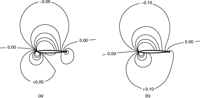
Figure 7.3.24 How the pressure distribution in the field around an airfoil is affected by a change in α, as illustrated by isobar patterns for a thin symmetrical airfoil (NACA 0010) at two angles of attack. Except for some differences due to thickness, doubling the angle of attack roughly doubles the strength of the pressure disturbances but does not much change the degree of “spreading” of the disturbances above and below the airfoil. Solutions calculated by the MSES code (Drela, 1993) in the inviscid mode. (a) α 4°, C_l 0.4761; Cp contour interval 0.05. (b) α 8°, C_l 0.9497; Cp contour interval 0.10

7.4 Airfoils

In the previous section, we defined an airfoil as a cross section of a wing of finite span. In the early years of the development of aerodynamics, this terminology was not yet standardized, and “airfoil” or “aerofoil” often referred to a complete 3D wing. Anderson (1997, pp. 288–289) provides an interesting look at the often-conflicting terminology that was used in the early days. In any case, in the previous section, we spent considerable effort just trying to explain how an airfoil produces lift, which is its primary purpose. Here we'll look into the many other important aspects of airfoils, including how pressure distributions and integrated forces depend on airfoil shape and angle of attack, factors influencing drag, factors influencing maximum lift, and considerations in airfoil design, including some specialized classes of airfoils.

7.4.1 Pressure Distributions and Integrated Forces at Low Mach Numbers

The pressure distribution on an airfoil surface, and the resulting integrated forces, over a wide range of flow conditions, can be predicted with good accuracy by computational fluid dynamics (CFD) calculations based on the NS equations or a coupled inviscid/viscous method. But for airfoils with nicely streamlined shapes at low Mach numbers and in the attached-flow regime, there are some general characteristics of the pressure distribution, the lift curve, and the pitching moment that we can predict without resorting to detailed flow solutions, but relying instead on a simplified linear theory. We'll begin this section by considering what the linear theory can tell us.

The linear inviscid theory was developed by Munk around 1920 (see the historical sketch by Giacomelli and Pistolesi, in Durand, (1967a) and formally applies in the limit of small thickness and angle of attack, but even for airfoils with practical amounts of thickness and camber, it is close enough to reality to provide useful insights. The beauty of the linear theory is that the effects of angle of attack, thickness, and camber can be treated separately and superimposed, which is not only computationally convenient, but provides a powerful way of thinking about how airfoil shape and angle of attack affect the pressure distribution.

In the linear inviscid theory, we assume incompressible potential flow and construct solutions by superposition of a uniform free stream and disturbances “produced” by elementary singularities. Superposition is allowed because the incompressible potential equation is linear to start with. To simplify the problem further we linearize the boundary conditions as well, which involves two things:

1. The flow-tangency boundary conditions that in higher-fidelity theories would be applied on the airfoil upper and lower surfaces as shown in Figure 7.4.1a, are applied instead along the x axis (y = 0), as shown in Figure 7.4.1b and
2. We ignore the longitudinal perturbation velocity u in calculating the velocity slope that is matched to the airfoil surface slope.

In keeping with applying the boundary conditions on the x axis instead of the airfoil surface, the sheet of distributed source strength and vorticity that “produces” the flow disturbance is also placed along the x axis. This sheet of singularity strength “causes” the perturbation velocities u and v to vary along the x axis and to have different values above and below the axis, which are taken to represent airfoil upper-surface and lower-surface values respectively. The equations that are solved for the distributions of source and vorticity strength are just the tangency condition illustrated in Figure 7.4.1b, imposed for both upper and lower surfaces, over the whole chord. The source and vortex singularities play complementary roles in influencing the perturbation velocities u and v. The averages and differences in the perturbations between the upper and lower surfaces are influenced differently, and the influence relationships are most easily illustrated in Table 7.4.1.

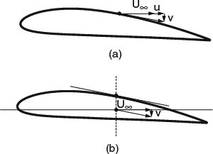
Figure 7.4.1 Flow tangency boundary conditions in airfoil potential flow, illustrated for the upper surface. (a) Full tangency condition applied at airfoil surface. (b) Linearized tangency condition applied on the x axis. Note that perturbation u is ignored

Table 7.4.1 Influence relationships in linear airfoil theory

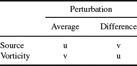
For the analysis problem (solving for the pressures for a given airfoil shape), we can decompose the airfoil surface slope into contributions from the angle of attack, the shape of the mean line, or camber line (halfway between the upper and lower surfaces), and the shape of the thickness distribution (the difference between the upper and lower surfaces), and we can then determine the first-order pressure coefficient C_p = −2u/U_∞ for each part separately, where u is the streamwise perturbation velocity evaluated on the chordline. These components of the geometry and their corresponding contributions to the pressure distribution are shown in Figure 7.4.2a–c for a NACA 4410 airfoil. Adding these pressure contributions together, we get a prediction for the complete pressure distribution of the airfoil, in Figure 7.4.2d. These plots follow the usual convention for plotting pressures in aerodynamics, with C_p plotted on an inverted scale so that when an airfoil is lifting upward, the pressure on the upper surface appears above the pressure on the lower surface.

The angle of attack and the mean-line shape affect only the average of the upper-and lower-surface slopes and thus the average v perturbation, and they therefore affect only the vorticity distribution, according to Table 7.4.1. As we saw in Section 3.3, the local strength of a vortex sheet is equal to the difference (jump) in tangential velocity across the sheet. In this case, the local strength of the vorticity distribution on the chordline is equal to the perturbation u and is therefore also proportional to the pressure difference, or the local lift loading.

The thickness shape affects only the difference in surface slopes and thus the difference in the v perturbations, which is locally equal to the strength of the source distribution. The source strength, and therefore the thickness distribution, affects only the average of the u perturbations, not the difference, according to Table 7.4.1.

So we see that according to linear theory, the chordwise distribution of lift is affected only by angle of attack and camber shape, not by thickness, and that the thickness shape affects only the average velocity over the upper and lower surfaces. This is reflected in the contributions to the pressure distribution shown in Figure 7.4.2. The pressure distributions due to angle of attack in part (a) and camber shape in part (b) are pure lift-carrying pressure differences (equal and opposite on upper and lower surfaces) with zero average perturbation pressures. The pressure distribution due to thickness in part (c) has a nonzero average and zero difference.

Now look in particular at the pressure distribution due to angle of attack, shown in Figure 7.4.2a for an angle of attack of 2°. Note that the shape of this pressure distribution is generic and that only the amplitude changes with angle of attack. The distribution is singular at the leading edge (ΔC_p is infinite), but it is integrable, and the lift and moment at a given α can be calculated by integration. Because the ΔC_p varies linearly with angle of attack, the lift slope dC_l/dα is constant, and its value is 2π per radian. The lift is concentrated well forward, and the centroid, or the point about which the pitching moment is zero, is located at the quarter chord for any nonzero angle of attack. The quarter chord is thus a convenient reference point for pitching moments: Any nonzero pitching moment about the quarter chord can be due only to the camber shape and will not vary with α, according to the linear theory. This holds true with reasonable accuracy for airfoils with practical amounts of thickness and camber, in the absence of nonlinear compressibility effects, and up to angles of attack at which boundary-layer separation begins.

Figure 7.4.2 NACA 4410 airfoil at 2° angle of attack, shown decomposed into a chord line, camber (mean line), and thickness. The linear-theory contribution of each to the pressure distribution is also shown. (a) Angle of attack. (b) Camber line (NACA 44xx). (c) Thickness shape (NACA xx10). (d) All combined for NACA 4410 airfoil at 2° α

The pressure distribution due to a typical camber shape at zero α is shown in Figure 7.4.2b, in particular the NACA 44xx mean line. This mean line produces an incremental C_l of 0.455 with its centroid at 0.488 x/c, for a pitching-moment coefficient C_m of −0.108 about the quarter-chord.

Figure 7.4.2c shows the pressure distribution for the NACA xx10 thickness shape at zero α, which is, of course, the same upper and lower. Combining this with the α and camber contributions, (a) and (b), gives the complete linear-theory pressure distribution for the NACA 4410 airfoil at 2° α, shown in part (d).

Linear theory can also be applied to the “inverse” design problem (solving for the airfoil shape for a given pressure distribution). Here we would decompose the pressure distribution into a lift part (difference between upper and lower pressures, as shown in Figure 7.4.2 by the sum of (a) and (b), and a thickness part (average of upper and lower pressures, as in Figure 7.4.2c). The lift part determines the mean-line shape and the angle of attack, and the thickness part determines the thickness shape. Linearized design is almost never used in practice, because anyone who really wants to design an airfoil will invariably want to use a higher-fidelity theory. We'll discuss airfoil design further in Section 7.4.10.

So to summarize what the linear theory leads us to expect regarding the pressure distribution and forces on an airfoil:

1. The pressure difference between the upper and lower surfaces, and thus the lift, is due primarily to the angle of attack and the shape of the mean line and is much less affected by the thickness distribution.
2. The pressure disturbance averaged between the upper and lower surfaces is due mainly to the thickness distribution and much less affected by angle of attack and camber.
3. The integrated lift is linear with α, and the lift slope dC_l/dα is close to 2π per radian.
4. The pitching-moment coefficient C_m about the quarter-chord is nearly constant with α.

As we'll see, these expectations hold up reasonably well, at least qualitatively, for airfoils of practical thickness at low Mach numbers in the attached-flow regime.

Now let's look at some of the ways “real” airfoil flows differ from the predictions of the linear theory. First, even before we add viscous effects, just moving the inviscid-flow boundary conditions from the x axis to the actual airfoil surface and taking perturbation u into account in the boundary conditions have effects that increase with thickness, camber, and angle of attack. In Figure 7.4.3, pressure distributions from the linear theory are compared with inviscid-flow calculations from the MSES code (Drela, 1993) for two airfoils that differ by a factor of 2 in thickness, camber, and a: NACA 2405 at 1°, and NACA 4410 at 2° (same case as in Figure 7.4.2). In both cases, the linear-theory underpredicts the pressure disturbances compared with the higher fidelity inviscid calculations, but much less so for the thinner airfoil than for the thicker one. The discrepancy seems to grow roughly quadratically with thickness, as one might expect for nonlinear effects. Still, the linear theory captures the general character of the pressure distributions.

Figure 7.4.4 compares the linear theory with inviscid MSES calculations for the NACA 4410 in terms of the change in the chordwise distribution of lift for a change in α from 0° to 2°. Here we see that the linear theory captures the general character of the distribution, except that the real airfoil, with its blunt-nosed thickness distribution, has no singularity at the leading edge.

Viscosity can have significant effects on the pressure distribution, through the boundary-layer displacement effect. In Figure 7.4.5a, the inviscid MSES calculation of Figure 7.4.3b is compared with a corresponding viscous calculation at the same angle of attack for a chord Reynolds number of 10 million, assuming laminar-to-turbulent transition close to the leading edge. The boundary-layer displacement effect, which is at its strongest by far on the upper surface near the trailing edge, reduces the effective angle of attack and aft camber of the airfoil, and changes the circulation, affecting pressures over the whole chord and noticeably reducing the lift. If the viscous solution is run so as to match the inviscid C_l instead of the inviscid α, the differences in the pressure distributions are reduced, as shown in Figure 7.4.5b. Note that due to the reductions in the effective camber and α, the viscous calculation requires a higher α to match the inviscid C_l. The effect of the higher α can be seen in the higher suction level on the forward upper surface.

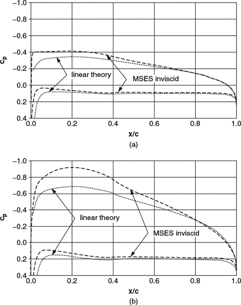
Figure 7.4.3 Comparison between the linear inviscid theory and incompressible inviscid flow with boundary conditions applied at the airfoil surface, calculated by the MSES code (Drela, 1993). Comparisons are made for two airfoil cases that differ by a factor of 2 in camber, thickness, and α, so that linear theory predicts a doubling of the pressure disturbances. (a) NACA 2405 at 1° α. (b) NACA 4410 at 2° α

The most dramatic local changes in pressure brought about by the boundary-layer displacement effect are seen in the neighborhood of the trailing edge. As we saw in Section 3.10, the inviscid flow off of a trailing edge with a nonzero wedge angle has a stagnation point, and the exact inviscid solution should thus have stagnation pressure (C_p = 1.0) at the trailing edge. The numerical solution plotted here doesn't reach stagnation pressure because the pressure change approaching the stagnation is too rapid to be resolved by the numerical grid (note that when a potential flow turns a concave corner of less than 90°, stagnation pressure is approached with infinite slope, as in Figure 3.10.2c). But this issue is irrelevant in the real world with viscous effects. Real pressure distributions look very much like the viscous solutions plotted in Figure 7.4.5, in which the boundary-layer displacement effect has substantially reduced the pressure recovery near the trailing edge and eliminated the stagnation. This alteration of the pressure distribution is a significant contributor to the profile drag, as we'll see later. It is easy to be deceived by appearances, however. Although the pressure changes near the trailing edge are the most dramatic, the pressure contribution to the profile drag is subtle and depends on changes around the entire airfoil contour.

Figure 7.4.4 The effect on the chordwise distribution of lift of a change in α from 0 to 2°. The linear-theory prediction, which is independent of airfoil shape is compared with a calculation for a NACA 4410 airfoil, calculated by the MSES code (Drela, 1993) in the inviscid mode

Now let's look at the effects of nonlinear boundary conditions and boundary-layer displacement on the lift-versus-α curve. Figure 7.4.6 shows the lift curve predicted by linear theory for the 44xx mean line, again showing the C_l shift of 0.455 at zero α and a slope dC_l/dα of 2π per radian. For comparison, MSES predictions are shown for the NACA 4410 and NACA 4420 airfoils, for both inviscid flow and all-turbulent flow at R 10 million. The inviscid MSES calculations show higher lift slopes than linear theory, increasing with increasing thickness ratio. The viscous calculations show significant losses of lift relative to inviscid. The calculation for 10% thickness ratio just happens to agree closely with the linear theory over the linear part of the lift curve, while the calculation for 20% thickness ratio is lower. At higher angles of attack, the displacement thickness of the boundary layer on the aft upper surface grows rapidly with angle of attack, causing the lift curve to become nonlinear and the lift slope to decrease. The maximum lift shown may be close to the maximum lift this airfoil could produce, but the MSES solution scheme based on simultaneous boundary-layer/inviscid-flow coupling did not in this case produce solutions showing maximum lift and beyond.

So far, we've seen two important effects of viscosity on the pressure distributions: The reduction in aft pressure recovery that contributes to profile drag, which we'll discuss in Section 7.4.2, and a reduction in lift slope that increases with increasing thickness. The latter effect explains what Yates (1990) referred to as the “fatness paradox,” in which the lift slope in inviscid flow increases with increasing thickness, while the lift slope in viscous flow decreases.

Figure 7.4.5 Effect of viscosity on the pressure distribution of NACA 4410 at 2° α, R = 10⁷, tripped to turbulent at 5% chord, calculated by the MSES code (Drela, 1993). (a) Inviscid and viscous MSES calculations at 2° α. (b) Inviscid MSES calculation at 2° α; viscous calculation matches inviscid C_l = 0.7385 (α = 2.541°)

In Figure 7.4.4, we saw that a rounded leading edge removes the leading-edge singularity that would generally occur in the inviscid solution for the mean line alone. On an airfoil that has no sharp corner other than the trailing edge, flow attachment occurs at a stagnation point, as we saw in Section 5.2.1. A stagnation point is, of course, a feature that the linear theory cannot model accurately. At moderate angles of attack for most airfoils, the stagnation point occurs near the leading edge. Figure 7.4.7 shows the pressure distribution plotted versus arc length around the leading edge, calculated for the NACA 4410 at an angle of attack of 2° in inviscid flow and at the matching C_l condition for viscous flow (same conditions as in Figure 7.4.5b). There is a slight shift in the location of the stagnation point, but the shape of the pressure distribution in the neighborhood of the stagnation point is affected very little by viscosity. The value of C_p at stagnation is greater than 1 because of numerical issues related to running a compressible code at a very low Mach number.

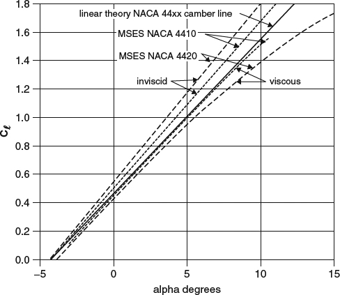
Figure 7.4.6 Lift curves predicted by linear theory and the MSES code (Drela, 1993) with and without viscosity for the NACA 4410 and 4420 airfoils

Figure 7.4.7 Pressure distributions in the neighborhood of the leading-edge stagnation point of a NACA 4410 airfoil. The inviscid MSES calculation is at 2° α, and the viscous calculation matches the inviscid C_l = 0.7385 (α = 2.541°, as in Figure 7.4.5b)

7.4.2 Profile Drag and the Drag Polar

In Chapter 6, we looked in considerable detail at drag in general, and we noted that although it is not possible to rigorously decompose the drag force according to the flow mechanisms that cause it, an approximate decomposition into lift-induced drag, shock drag, and viscous drag is possible with the aid of simplified theoretical models. The problem we face here is simpler: A 2D airfoil in 2D flow has no induced drag, and shock drag appears only at transonic speeds when regions of supersonic flow appear in the field. We'll defer transonic issues to Section 7.4.8 and look now just at the viscous drag in subcritical flow. As we saw in Section 6.1.3, viscous drag has both a shear component and a pressure component. In the context of airfoils and wings, the viscous drag is often called the profile drag.

Of course in an ideal 2D inviscid flow without shocks, the drag of an airfoil must be zero. This is an example of D'Alembert's paradox, which we discussed in Sections 5.4 and 6.1.6. Intuitively speaking, zero drag is even more surprising in the case of a lifting airfoil at an angle of attack than it is in general. Consider the lifting airfoil sketched in Figure 7.4.8a. Because of the general downward slope of the airfoil surfaces, due to the angle of attack, the pressure difference between the upper and lower surfaces produces a net force that over much of the airfoil chord is tilted backward as illustrated by the arrow above the airfoil. If the integrated pressure force over so much of the chord is tilted backward, how can the drag be zero? The answer to this lies with something that is loosely termed leading-edge suction. On a lifting airfoil with a rounded leading edge, as in Figure 7.4.8a, the pressure around the leading edge is predominantly lower than elsewhere, as indicated by the minus signs, just enough to balance the general backward tilt of the lift over the rest of the chord. On an airfoil with zero thickness, as in Figure 7.4.8b, there is only one angle of attack at which the flow attaches smoothly to the leading edge. At any other angle of attack, the potential flow around the leading edge has a singularity with infinite velocity, and produces a singular suction force parallel to the surface tangent at the leading edge, as indicated by the arrow. In 2D inviscid flow, this suction force must exactly cancel any net drag force resulting from the pressure differences over the rest of the chord.

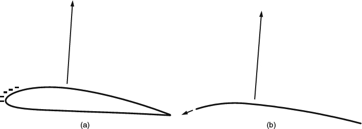
Figure 7.4.8 The concept of leading-edge suction. (a) Low pressure around a rounded leading edge. (b) Singular suction force at the leading edge of an airfoil with zero thickness

In the real world, the viscous drag of a typical streamlined airfoil in attached flow tends to be small, on the order of 10⁻² in terms of the drag coefficient. When we want to predict airplane performance or compare candidate designs, we would like to pin this small drag number down to within a small percentage, so we are looking at trying to predict the profile drag to within something on the order of a drag count (10⁻⁴). Computational predictions at this level are at or beyond the limit of what is currently practical and are therefore problematic. When we are looking at increments on the order of a drag count, we should use only the best methods available, and we should apply them with great care. We'll address the CFD issues further in Chapter 10. Experimental measurements of drag at this level are likewise difficult. Only particular experimental setups and measurement methods are up to the task, and then only marginally so. Experimental uncertainties are often as large as the increments we would like to determine. These difficulties, however, don't keep us from drawing some general conclusions about the nature of viscous profile drag.

In Section 5.4 and in Section 6.1.3, we discussed the decomposition of drag into a surface shear stress, or skin-friction part and a pressure part, and noted that this decomposition involves none of the theoretical idealization that is required in the induced/shock/viscous drag decomposition. In attached flow, typical airfoil profile drag is mostly integrated skin friction, but pressure also makes a significant contribution, as a result of the boundary-layer displacement effect. A viscous-inviscid interaction code can do a reasonable job of predicting the boundary-layer displacement thickness, but an NS code is generally required if one is to calculate the effect on the pressure accurately enough to allow the viscous pressure drag to be calculated by direct pressure integration. In practice, accurate prediction of the pressure drag in an NS code requires a flow solution with an excellent degree of grid convergence. In viscous-inviscid interaction codes, the pressure drag cannot generally be calculated directly with sufficient accuracy, and the total drag must be inferred from less-direct flowfield manifestations. The wake development can be calculated into the farfield and used in the farfield wake-momentum formula, Equation 6.1.7, as is done in the MSES code (Drela, 1993), for example, or trailing-edge boundary-layer quantities can be used in the Squire-Young formula, Equation 6.1.8 for incompressible flow, or the compressible version by Cook (1971).

Now let's look at typical behavior of skin-friction and pressure drag, using MSES calculations for the NACA 4410, the airfoil whose pressure distributions we looked at in Figure 7.4.5. First, a typical distribution of C_f along the chord is shown in Figure 7.4.9, for the same flow condition as in Figure 7.4.5b. Flat-plate C_f from Equations 4.3.4 and 4.3.5 is shown for comparison. The artificially forced transition from laminar to turbulent at 5% chord is clearly seen. It is also clear that pressure gradients and edge velocities different from freestream make C_f on the upper and lower surfaces considerably different from that on a flat plate, and that C_f on the upper surface is higher than that on the lower surface, except near the trailing edge. In Figure 7.4.10 we look at the drag polar behavior, that is, how these things vary with C_l. The skin friction calculated by the code's boundary-layer equations was integrated directly, and the total drag was calculated from the farfield wake momentum. The difference was assumed to be the pressure drag and labeled as such. The total skin-friction drag is only slightly greater than that on a two-sided flat plate and varies little with C_l. Most of the variation of the drag with C_l is seen to come from the pressure drag. The variation is roughly parabolic at lower C_l, but it becomes strongly nonparabolic at higher C_l, as the boundary layer on the aft upper surface approaches separation.

Figure 7.4.9 Skin-friction distribution for NACA 4410 calculated by the MSES code (Drela, 1993). R = 107, C_l = 0.7385 (α = 2.541°). Here C_f is normalized by farfield q, not local edge q. C_f for a flat plate at the same Reynolds number is shown for comparison

In Section 6.2.1, we discussed the concept of a form factor that relates the actual profile drag to the skin-friction drag of a flat plate at the same chord Reynolds number and with laminar-to-turbulent transition at the same chord location. Handbook methods for drag estimation often use the form factor in estimating the profile drag of the airfoils that make up the wing. The flat-plate skin friction is easily calculated by Equation 4.3.2 for all-turbulent flow, and an adjustment can be made if a significant run of laminar flow is expected. The form factor itself poses more of a problem and is thus the weak point of the form-factor approach. To illustrate why, the form factor variation calculated from the MSES predictions of Figure 7.4.10a is plotted in Figure 7.4.10b. Like the pressure drag in Figure 7.4.10a, the form factor has a roughly parabolic variation at lower C_l and becomes strongly nonparabolic at higher C_l. Note that even at the drag minimum the form factor is greater than 1 by more than 20%, reflecting the fact that the viscous drag of an airfoil is typically significantly greater than the skin-friction drag of a flat plate. In handbook methods, only the parabolic part can be correlated reasonably well with the airfoil maximum thickness and maximum camber. The nonparabolic part depends on airfoil design details and is usually ignored. As a result, when it comes to making airplane performance predictions, relying just on the parabolic part of the airfoil polar that fits the low-C_l range is bad practice. Usually, the airfoil C_l that provides the highest airplane lift/drag ratio is determined by the rapid increase in profile drag on the nonparabolic part of the airfoil polar. Using the parabolic polar that fits the low-C_l range will generally lead to a choice of operating C_l that is too high and will also yield a seriously optimistic drag estimate.

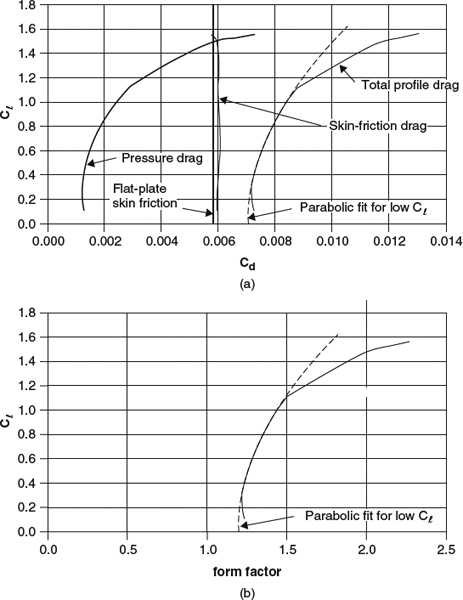
Figure 7.4.10 Drag predicted by the MSES code (Drela, 1993) for the NACA 4410, R = 10⁷, at 5% chord. (a) Drag polar. (b) Form factor

7.4.3 Maximum Lift and Boundary-Layer Separation on Single-Element Airfoils

We now turn our attention to the problem of the maximum lift an airfoil can produce and how it is affected by the airfoil shape and pressure distribution. There are limits to the amount of lift that can be produced even in inviscid flow, as discussed by Smith (1975). Either the circulation becomes so large that the attachment and separation points merge, and it is assumed that larger circulation would be a mathematical artificiality, or the condition on the upper surface approaches vacuum. Smith points out that these limits are moot, however, because viscous effects impose much lower limits. As we noted in our basic explanation of lift in Section 7.3.3, the maximum lift of an airfoil is limited because “there is an angle of attack above which the flow cannot follow the upper surface and breaks away,” as shown in Figure 7.3.16. Now it's time to look in more detail at what that means. The breaking away is of course boundary-layer separation, and it changes the basic topology of the flow, as we discussed in Sections 5.2 and 5.3. As we saw in Section 4.1.4, the immediate cause of any separation from a smooth surface in 2D flow must be an adverse pressure gradient. The angle of attack strongly affects the pressure distribution and is therefore a primary variable affecting separation. Separation also depends on the Reynolds number and the location of laminar-to-turbulent transition.

The progression of separation with angle of attack, and the resulting variation of lift with angle of attack, can follow a variety of scenarios, depending on the details of the airfoil shape and pressure distribution and on whether the boundary layer is laminar or turbulent at the separation point. We'll take a brief look at the interesting complexities that can accompany laminar separation before we take up the simpler case of turbulent separation that dominates at high Reynolds numbers.

If the Reynolds number is relatively low, or if the airfoil is thin enough, separation can often occur while the boundary layer is still laminar, and the progression with angle of attack can be complicated. The shear layer downstream of a laminar separation is generally highly unstable, and transition tends to happen within a short distance, but of course the distance depends on the Reynolds number. Depending on the length of the transition region and the shape of the airfoil, transition may or may not cause reattachment of the boundary layer to the surface. A laminar separation with subsequent turbulent reattachment is called a laminar separation bubble and generally has the structure illustrated in Figure 7.4.11. If the displacement-thickness Reynolds number at the separation point is above 500 (see Thwaites, 1958), transition is very quick and nearly always results in reattachment. The resulting bubble is typically only 1–2% of the chord in length and is called a short bubble. At lower Reynolds numbers, transition is less vigorous, and reattachment may or may not occur. If a bubble results, it is referred to as a long bubble.

Figure 7.4.11 General structure of a laminar separation bubble with turbulent reattachment. From Thwaites, (1958). Used with permission of Dover Publications, Inc.

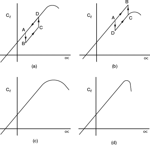
Figure 7.4.12 Lift curves showing different types of stall behavior depending on the progression of upper-surface boundary-layer separation. (a) Counter-clockwise hysteresis loop in the mid-C_l range associated with laminar separation near mid-chord. (b) Clockwise hysteresis loop at the top of the lift curve associated with the bursting of a laminar separation bubble near the leading edge. (c) Gentle turbulent stall: separation moves forward gradually, and lift increases somewhat after the first appearance of separation. (d) Sudden turbulent stall: separation jumps forward suddenly, and lift increases little or not at all after first separation

Most airfoil flows are unique, in that there is only one possible flow pattern for a given airfoil shape, farfield flow condition, and angle of attack. But in some situations when laminar separation bubbles are involved, there can be two possible flow patterns at the same angle of attack, and the lift curve can have a hysteresis loop. Figure 7.4.12a,b shows two possible types of hysteresis loop.

The counterclockwise loop in part (a) is associated with a laminar separation bubble near mid chord that first appears at an angle of attack below point A. As point A on the lift curve is approached from below, the boundary layer ceases to reattach, and the lift jumps down to point B on the lower branch. When the angle of attack is further increased to point C, transition moves ahead of the former separation point, the separation disappears, and the lift jumps up to point D. When the loop is traversed in the other direction, earlier transition continues to prevent the laminar separation, and the lift follows the upper branch back to point A.

A clockwise hysteresis loop like that shown in part (b) of Figure 7.4.12 is more common and is associated with laminar separation near the leading edge. Below point A on the lift curve, there is a laminar short bubble with reattachment. The laminar bubble thickens the boundary layer considerably, however, and reduces the turbulent boundary layer's ability to resist separation downstream. (We'll look at the effect of incoming boundary-layer thickness on turbulent separation in some detail in connection with turbulent stall below.) At point B, separation jumps forward suddenly from the trailing edge to the leading edge, leading to the precipitous drop in lift to the lower branch at point C. This is often described as the “bursting” of the laminar bubble. Now that the lift is reduced, and with it the circulation around the airfoil, the stagnation point is not as far aft on the lower surface as it was when the lift was on the upper branch. The distance around the leading edge from stagnation to separation is shorter, the displacement-thickness Reynolds number at separation is lower, and the ability to reattach is reduced. As angle of attack is reduced, the lift follows the lower branch to point D before the reattachment is reestablished, and the lift jumps back up to point A.

Obviously, flows with laminar separation bubbles can display complex behavior, and it turns out that they are not that easy to predict. Drela's ISES and MSES codes, which are based on viscous/inviscid interaction, and in which the integral-boundary-layer portion of the analysis includes a transition-prediction module, can predict such flows in some cases. At the current state of the art, NS codes based on the RANS equations with turbulence modeling don't routinely predict these effects because they don't typically incorporate any option for transition prediction.

At the high Reynolds numbers typical of large airplanes, laminar separation tends not to arise, and lift is limited by turbulent separation. In a “turbulent stall,” lift can increase substantially or very little after separation first appears, depending on how the separation moves forward as angle of attack increases. As a result, the airfoil's lift curve can vary between the extremes illustrated in Figure 7.4.12c,d. Separation may move gradually forward from the trailing edge, producing a gradual reduction in lift slope and a broad maximum in the lift curve as in part (c), or it may jump forward suddenly, producing a precipitous drop in lift as in part (d). In the gradual scenario, the actual stall, or onset of the decrease in lift, is usually preceded by buffeting caused by flow unsteadiness related to the separation, and the loss of lift post-stall is gradual. In the sudden scenario, the stall comes without warning, and the loss of lift is abrupt, which can cause sudden changes in airplane handling characteristics. Obviously, flight safety favors a gradual stall, and we'll see later what pressure-distribution features can be designed into an airfoil to produce it. Even an airplane with a gradual stall, however, is deliberately flown into the buffeting regime only in special circumstances, typically flight testing and pilot training, and in this sense, the onset of flow separation provides one definition of the maximum usable lift coefficient. For this reason, and because it is easier to predict computationally than the actual maximum lift, we'll take the onset of flow separation as the threshold for purposes of this discussion.

By this criterion, the maximum lift depends on how low the average upper-surface C_p can be made before the upper-surface boundary layer can no longer make it to the trailing edge without separating. The “run” of the upper-surface boundary layer starts at the stagnation point of attachment, which under high-lift conditions is usually on the lower surface, back a short distance from the leading edge, so that the boundary layer must flow around the leading edge before it starts to traverse the upper surface. Then whether the boundary layer separates or not depends on the pressures it is subjected to around the leading edge and along the entire upper surface.

We saw what a typical upper-surface pressure distribution looks like in Figure 7.4.2: There is a decrease in pressure as we move away from the stagnation point of attachment near the leading edge, and a minimum pressure we'll call the suction peak, which can be very close to the leading edge or farther back, depending on the airfoil shape and the angle of attack. The suction peak is followed by an increase in pressure, or pressure recovery from the suction peak to the trailing edge. For an airfoil with nonzero thickness in attached viscous flow, the C_p at the trailing edge typically has a slightly positive value that depends primarily on the average thickness and is not very sensitive to the details of the thickness shape, for reasonable shapes.

The recovery region is where the pressure gradient is adverse, and that's where we'll concentrate our attention. In general, a streamlined body with thickness in attached flow must have a recovery region at the rear. In Figure 7.4.2c, we saw that a typical airfoil thickness distribution by itself contributes a modest amount to the recovery, and in Figure 7.4.2b, we saw that the typical camber distribution also contributes. For determining maximum lift, the contribution from angle of attack (Figure 7.4.2a) is crucial because it increases with angle of attack, making the pressure gradient over the entire recovery region increasingly adverse. Increasing α eventually causes the gradient to exceed what the boundary layer can tolerate, regardless of other details of pressure distribution.

To maximize the lift at the onset of separation, we want to make the average C_p on the upper surface as negative as possible, subject to the constraint imposed by the slightly positive C_p that we must reach at the trailing edge. We can decrease the average C_p either by lowering the minimum pressure or by keeping the pressure low over more of the chord, which delays the start of the recovery, or by a combination of both. Lowering the minimum pressure increases the pressure rise the boundary layer must withstand. Delaying the start of the recovery shortens the distance in which the recovery must take place and thickens the boundary layer at the start of the recovery, both of which tend to bring separation on sooner. The shape of the recovery pressure distribution is also an important factor.

There is no single, simple way to visualize how all of these factors come together to affect maximum lift. A conventional C_p plot normalized by the farfield dynamic pressure q_∞, has the advantages of directly showing the effects of the pressure distribution on C_l and of making it clear that all recovery pressure distributions are essentially “anchored” to a trailing edge C_p that is fixed within a narrow range. But conventional C_p at the suction peak varies widely, making it difficult to visualize how that part of the pressure distribution affects separation. The amount of pressure rise, or velocity drop, that the boundary layer can withstand is much more closely related to the conditions at the suction peak than to those in the farfield. In his classic Wright Brothers lecture on high-lift aerodynamics, Smith (1975) suggested that plotting recovery pressure distributions in what he called canonical form, in terms of a pressure coefficient relative to the suction-peak pressure and normalized by the peak dynamic pressure, reduces the variation in ΔC_p between the suction peak and separation and makes the separation trends easier to see. The canonical pressure coefficient is thus defined and related to conventional C_p by

where the subscript o denotes conditions at the suction peak, which we'll take as the start of the recovery. Note that at the suction peak is zero by definition, and it takes on only positive values in the recovery. Separation of a turbulent boundary layer generally occurs at values between 0.4 and 0.9, a much smaller range than we would see in terms of conventional ΔC_p. Of course, to see how the separation trends affect C_l, we will still have to return to the conventional pressure distribution.

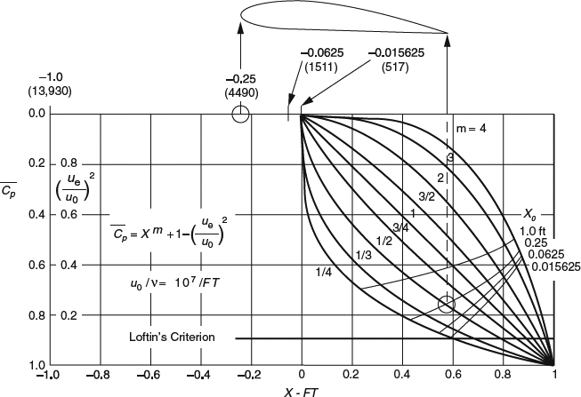
Figure 7.4.13 Separation loci for a family of power-law canonical pressure distributions preceded by different lengths x₀ of boundary-layer run ahead of the recovery. In parentheses are values of R_θ at x = 0. (From Smith, 1975; Figure 20.) The airfoil sketch at the top, and the circles and arrows pointing to it, were added to Smith's original figure to illustrate how these curves would apply to a hypothetical airfoil for the particular case of x_o = 0.25 ft and m = 1/2

Let's look at some separation trends in terms of canonical pressure distributions. Figure 7.4.13, from Smith (1975), shows in a single plot how at separation is affected by the shape of the recovery pressure distribution and the thickness of the boundary layer at the start of the recovery, which in these examples is determined by the length x_o of an ideal constant-pressure boundary-layer run ahead of the start of the recovery. The longer the length x_o, the thicker the boundary layer at the start of the recovery. The results shown are for turbulent boundary layers and are based on numerical solutions to the boundary-layer equations with the algebraic eddy-viscosity model of Cebeci and Smith (1974) and with the given pressure distributions as boundary conditions. Because of the limitations of the simple turbulence model, these calculations are generally optimistic regarding to the amount of pressure recovery that is possible, especially in the cases where the recovery leading to separation is short when measured in terms of initial boundary-layer thicknesses, but the qualitative trends are realistic.

Three important trends are clear in Figure 7.4.13:

1. A concave recovery (a recovery pressure distribution characterized by m < 1, in which the adverse pressure gradient starts out strong and eases downstream) leads to separation in a shorter distance than does a convex recovery (m > 1),
2. In spite of the shorter distance to separation, a concave recovery produces greater pressure recovery than a convex recovery, and
3. A thin boundary layer at the start of the recovery (small x_o) results in greater pressure recovery, and a thick boundary layer results in less.

Smith (1975) showed that these results are not very sensitive to Reynolds number: Reducing the Reynolds number by a factor of 10 reduced the values of at separation generally by less than 0.1. But for a given pressure distribution, separation is strongly affected by wing sweep, as we'll see in Section 8.6.2.

So viewing recovery pressure distributions in canonical form makes it easier to visualize how the initial boundary-layer thickness and the shape of the pressure distribution affect separation. But it isn't clear just from the canonical distributions what these boundary-layer separation trends imply regarding airfoil maximum lift. To visualize the effects on maximum lift, we must convert the canonical distributions back to conventional form and view them as candidate upper-surface pressure distributions of a hypothetical airfoil with a rapid flow acceleration near the leading edge and a region of constant pressure back to the recovery point, followed by the pressure recovery.

The conversion to a conventional pressure distribution goes as follows. We take x_o in the canonical plot to correspond to the leading edge of our airfoil, and if we place the trailing edge at x_sep in the plot, we have separation beginning just at the trailing edge, which corresponds to our criterion for the maximum usable lift. The airfoil sketch at the top of Figure 7.4.13, and the circles and arrows pointing to it, were added to Smith's original figure to illustrate how this would work for a hypothetical airfoil in the particular case of x_o = 0.25 ft and m = 1/2. In this case the leading edge lines up with x = −0.25 ft, and the trailing edge lines up with x_sep for m = 1 /2, x_o = 0.25. For general cases, each of the possible combinations of x_o and x_sep then corresponds to particular locations of the leading and trailing edges on the plot, and a particular chordwise location x/c for the start of the recovery, often referred to as the recovery point. Then we assume that the conventional C_p at the trailing edge always has a slightly positive value, say 0.2, and that this corresponds to at separation for the particular pressure distribution we're considering in the plot. Through Equation 7.4.1, this defines u_∞ for each case we consider, and thus defines the relationship between and C_p. When we do this for any one of the canonical pressure distributions in Figure 7.4.13, and repeat it for various combinations of x_o and x_sep, we get a family of conventional pressure distributions with different recovery points and different C_p levels at the suction peak. Strictly speaking, each of these pressure distributions corresponds to a different chord Reynolds number, because in Figure 7.4.13 it is the “unit” Reynolds number u_o/v of the canonical x scale that is constant. But the Reynolds-number sensitivity is fairly weak, and this discrepancy shouldn't seriously distort the qualitative trends we're looking for.

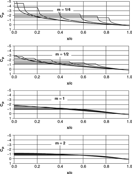
Figure 7.4.14 Families of conventional maximum-lift pressure distributions corresponding to some of the canonical pressure distributions of Figure 7.4.13; for each assumed location of the recovery point, the rooftop level was determined so that separation is reached at the trailing edge. All-turbulent flow was assumed ahead of the recovery

Results of this process are shown in Figure 7.4.14 for four of the canonical pressure distributions ranging from concave to convex. Several important trends are evident in these plots:

1. In the part of the pressure distribution ahead of the pressure recovery (often called the rooftop), higher suction levels (lower pressures) are possible with concave recoveries,
2. For a given shape of the recovery pressure distribution, the allowable suction level increases as the recovery point is moved forward, and
3. For a given suction level, a concave recovery allows a farther-aft recovery point and a longer rooftop.

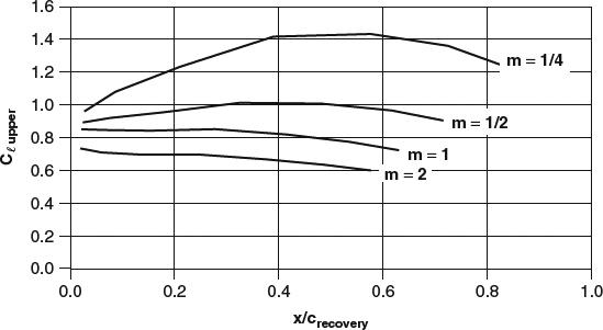
Figure 7.4.15 Upper surface C_l values for the pressure distributions of Figure 7.4.14, plotted versus the recovery-point location

A higher suction level and a longer rooftop both increase lift, so that in view of items (1) and (3) above, concave recoveries should be favorable. This is born out by the plots in Figure 7.4.14, which clearly show that concave recoveries produce higher lift, and by the corresponding upper-surface lift coefficients plotted in Figure 7.4.15.

It is also clear that for any given shape of recovery pressure distribution, high lift involves a compromise between having low pressure at the suction peak and having the low pressure extend over more of the chord. There is therefore an optimum location for the recovery point that yields the highest lift. Figure 7.4.15 shows that the optimum recovery point moves aft, and the maximum lift dramatically increases, as the recovery pressure distribution is made more concave. Remember that chord Reynolds number was not kept constant in these examples, and the trends are only qualitative approximations to what would happen for constant Reynolds number.

So in these examples, the highest maximum lift is achieved by the most concave recovery pressure distribution, or the most “rapid” recovery. Smith (1975) concluded that the highest possible lift that can be achieved without separation is achieved by the most rapid of all possible recoveries, the Stratford recovery (Stratford, 1959a, b), which is shown in canonical form in Figure 7.4.16 (Smith's Figure 21). In a Stratford recovery, an extremely strong pressure gradient at the start brings the boundary layer immediately to near-zero C_f, and the remainder of the pressure distribution is tailored to maintain the boundary layer in a constant state of incipient separation. The boundary-layer velocity profile in a Stratford recovery is nearly self-similar, and it is one of the family of equilibrium turbulent-boundary-layer flows that we discussed in Sections 4.3.2 and 4.4.2.

The potential for high maximum-lift coefficients led Liebeck (1973) to use the Stratford recovery pressure distribution as the basis for several low-speed airfoil designs. A drawback to this approach is that above the “design” angle of attack, separation jumps forward abruptly from the trailing edge, leading to the problem of abrupt stall that we've already discussed. As a result, Stratford-recovery airfoils have not found much application in aeronautical practice. Instead, designers developing airfoils for practical applications purposely back away from the Stratford recovery by varying amounts, that is, they make the recovery less concave, depending on how gentle they want the stall to be and how much of a penalty in maximum lift they are willing to pay for it.

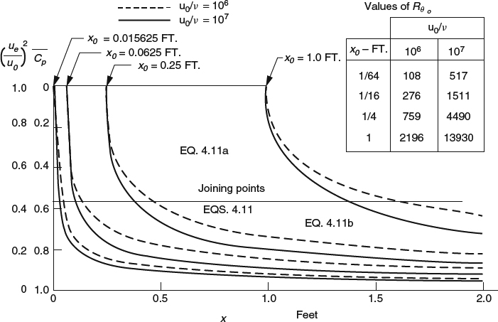
Figure 7.4.16 Canonical pressure distributions for Stratford's recovery at two different values of unit Reynolds number. (From Smith, 1975; Figure 21; including references to his equation 4.11)

So far we've assumed that the boundary-layer development is all-turbulent from near the leading edge, a situation Smith referred to as a turbulent rooftop. Now let's look at the case of a laminar rooftop. A run of laminar flow ahead of the start of the recovery, that is, a laminar rooftop, will result in a thinner boundary layer at the start of the recovery than would be there if the boundary layer were all turbulent. In terms of the canonical pressure distributions in Figure 7.4.13, we saw that a thin boundary layer at the start of the recovery tends to delay separation. In terms of the conventional pressure distribution, as in Figure 7.4.14, the thinner boundary layer would allow either a higher suction level in the rooftop or a longer rooftop, either of which would increase maximum lift. Figure 7.4.17, from Smith (1975), illustrates this effect by comparing conventional maximum-lift pressure distributions with laminar and turbulent rooftops. These examples happen to show Stratford recoveries, but the effects of a laminar rooftop are reasonably generic. For a given recovery-point location, a laminar rooftop allows a higher suction level, and for a given suction level, a laminar rooftop allows a longer rooftop. In view of the potential for very high maximum lift coefficients, Liebeck (1973) assumed a laminar rooftop for several of his airfoil-design examples. For practical applications, a drawback to designing an airfoil for a laminar rooftop at the maximum-lift condition is that if the airfoil surface becomes contaminated, say by rain or insects, and the flow trips early to turbulent, the maximum-lift capability will be greatly reduced.

Figure 7.4.17 Conventional maximum-lift pressure distributions with Stratford recoveries at a chord Reynolds number of 5 million. (From Smith, 1975; Figures 24 and 25.). (a) Laminar rooftop. (b) Turbulent rooftop

To summarize, we've seen that high maximum lift in a single-element airfoil favors concave and even Stratford-recovery pressure distributions, and a laminar rooftop. In airplane applications, however, such features are to be avoided for handling characteristics and safety reasons, and besides, single-element airfoil design is usually dominated by considerations in other parts of the flight envelope. For many airplanes, maximum lift for takeoff and landing is enhanced by high-lift devices with slots, which brings us to our next topic.