
5. Setting Up Your Character
Setting up a digital character involves two main steps: mechanical setup and deformation setup. I'm not talking about modeling or lighting, but about motion setup or rigging, which is the action of making a character controllable or poseable. Mechanical setup involves creating the skeleton that will drive the character and other skeletons that will be used to add motions of different types, as well as creating all the controls that will be used to animate the character. Deformation setup defines the relationship of each vertex of the character to the skeleton.
This chapter deals only with mechanical setup, because deformation setup is very specific to each particular software package and is implemented in the same way for both keyframed and captured motion data. Nevertheless, when using captured motion data, you must keep in mind that deformations are pushed to the limit. Thus, it is very important to take extra care when creating the mechanical setup that will drive them. Usually, the rotational data that a motion capture studio delivers is not enough to drive a typical vertex-weighting deformation scheme. Keyframe animators can distribute transformations across several joints when posing a character; for example, in twisting an arm, rotations can be partially added to the shoulder, elbow, and wrist in such a way that the character's envelope will not be twisted. Captured motion data does not follow this distribution pattern, but rather behaves in an anatomically correct way, assigning most of the twisting to the segment between the elbow and the wrist. This is usually not friendly to most deformation schemes. Setting up the mechanics of a character to follow the properties of the actual raw data is the key to better deformations.
The rotational motion data formats that were discussed in Chapter 4 include a skeleton for the user. In those cases, the mechanical setup has already been done for you. All you need to do is import the file and, voilà, a skeleton is readily available for your character. I question most of these file formats because the creation of a skeleton is not something to take lightly. In some cases, the default skeleton in the motion file will do, but the highest quality jobs will require a very careful mechanical setup that can only be designed by the same person who is responsible for the setup of the deformations.
To maximize your control over captured motion data, it is best to obtain the data in the simplest format possible. All you need is the tracked marker data, so the translational file will do. This file contains only a stream of marker position coordinates over time. By using this file, you can design the skeleton inside your animation environment and not abide by what a motion capture studio delivers. This method is definitely more time consuming, so make sure you also obtain the rotational data, and determine first if it is of adequate quality and if the skeleton is appropriate enough for your project.
Setting up a Character with Rotational Data
When rotational data is used for motion capture, a skeleton is already included or assumed by the data stream. It is possible that all you need to do is import the data into your software and your character will start moving. It is also possible that the data may be incompatible with your software, or that you may have to change your software's settings in order to receive the data.
Depending on the software used, you may have to create a skeleton before importing the data. If you are dealing with data in the Acclaim format, chances are you only need to load the .asf file. When using other formats, you sometimes have to create the skeletal nodes and then load the data to pose them. If you must do that, you need to find out what the initial orientation and position of the bones should be.
If you load a skeleton in its base position and its pose doesn't match that of the character, the ideal solution is to pose the character to match using the modeling software, but in most cases this is impossible. Another solution is to modify the base position to match the pose of the character. Doing so entails recalculating all the motion data to compensate. A third and most frequently used solution is to add an expression that will add an offset to the data equal to the negative of the offset added to the base position. This is almost equivalent to recalculating all the data, but it is done on the fly. This technique has the advantage of being quick and easy, but it is a hack after all, so it isn't the cleanest solution and may even complicate Euler angle problems that had previously been fixed in the data.
When you import rotational data into animation software, you must make sure that the data is prepared to transform your character in the same order as the software does. In some programs, you are able to change this order—sometimes for each segment or for the whole project. Others are not so flexible. Some programs allow you to change the order of rotations only, whereas others allow you to change when translations, rotations, and scaling happen. You need to know what your particular software supports before preparing the rotational data.
Most programs and motion data formats assume translations will happen before rotations, and scaling will happen after rotations. Most problems that arise usually concern the order of rotations specifically. Three-dimensional rotations are noncommutative, which means you cannot interchange their order and obtain the same result.
A program that is used in a lot of pipelines is Autodesk MotionBuilder. This software primarily works with raw data but it will deliver rotational data in a skeleton for use in 3D animation packages such as Maya or video game engines.
Setting up a Character with Translational Data
The files you use to set up a character with translational data contain a set of markers with positional coordinates over time. You use combinations of these markers to create approximations of rigid segments that will define the skeleton of your character.
Creating the Internal Skeleton
The first step in setting up the character is finding the locations of all the local coordinate systems that will represent the new internal skeleton. There is at least one coordinate system associated with each of the rigid segments, and you need to find equations or formulas that will allow you to find these over time. Once you have these formulas, you can use them in your animation or video game software to position and orient joints.
The bones can be calculated using exclusively the markers that define the rigid segments associated with them, or you can use previously found internal points in combination with markers. The latter approach makes the process easier and ensures that the segments are linked to each other, considerable inaccuracy being common because markers are placed on the skin and do not exactly maintain their position relative to the bones.
Center of Gravity
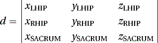
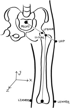
The location of the character's center of gravity must be determined. Assuming the data was captured using the default marker setup defined in Chapter 3, the pelvis segment is defined by the SACRUM, LHIP, and RHIP markers. Figure 5.1 is a visualization of the center of gravity, shown in the figure as point PELVIS(xPELVIS, yPELVIS, zPELVIS).
 |
| Figure 5.1 The center of gravity. |
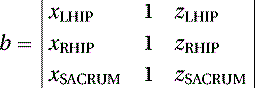
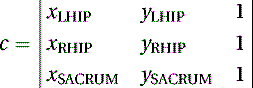
We begin by defining the rigid segment formed by SACRUM, LHIP, and RHIP, using the following linear equation of a plane: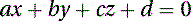
(5.1)
As we know the coordinates of three points in space, LHIP(xLHIP, yLHIP, zLHIP), RHIP(xRHIP, yRHIP, zRHIP), and SACRUM(xSACRUM, ySACRUM, zSACRUM), the constants (a, b, c, and d) of Equation (5.1) can be calculated by the following determinants: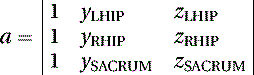
(5.2)
(5.3)
(5.4)
(5.5)
We can expand these equations, obtaining the following:


(5.6)
(5.7)
(5.8)
(5.9)
We then proceed to find the direction cosines (σx, σy, σz) of the normal N of the plane as follows:
(5.10)
(5.11)
(5.12)
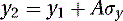
We continue by defining a line segment L between points LHIP and RHIP. We will refer to the midpoint between LHIP and RHIP as P1 and will calculate its coordinates by using the following linear parametric equations:
(5.13)
u is the parametric variable that defines where in the line the point is located. Substituting u = 0, we obtain the coordinates of one of the end points; with u = 1, we obtain the coordinates of the second end point. u = 0.5 will give us the coordinates of P1, the midpoint in the center of the line segment.
As we know the coordinates of the end points LHIP and RHIP, to solve the equations we start by substituting the end point coordinates. For the first end point, we assume u = 0 and we obtain where xLHIP, yLHIP, and zLHIP are the coordinates of marker LHIP. For the second end point, we substitute u = 1 and obtain
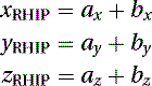
(5.14)
(5.15)
Finally, we substitute Equations (5.14) and (5.16) into Equation (5.13) and obtain the coordinates of P1(x1, y1, z1), where u = 0.5:
(5.17)
Next, we need to calculate the constant length of line segment A; to do so, we will need to assume that the system is in a base pose where L is aligned with the world x-axis and A is aligned with the world y-axis. In this state, we can further assume the following:
(5.18)
We make these assumptions because when the system is in its base state, PELVIS is located at the same height as SACRUM and at the same width and depth as P1. The length of A is then calculated by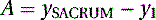
(5.19)
We have a line segment B from P1 to P2 that is parallel to N and of equal length to A. We know that any two parallel lines in space have the same direction cosines, so the direction cosines of B are the same as the direction cosines of N. The direction cosines for B are computed using the following equations:


(5.20)
(5.21)
(5.22)
As the only unknown variables are x2, y2, and z2, we can obtain the frame-by-frame location of P2 as follows:

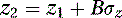
(5.23)
(5.24)
(5.25)
Next, we need to find the value of θ, the angle between the plane normal and the z-axis. We know that so for a base pose, we can calculate θ by
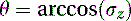
(5.26)
(5.27)
The angle α between A and B is then found by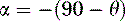
(5.28)
To find the location of PELVIS, we need to rotate P2α degrees about the local x-axis at P1. We perform this operation by first translating P1 to the origin, then performing the rotation in x, and finally reversing the translation. We achieve this by the following set of matrix transformations: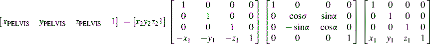
Vertebral Column
The vertebral column's four segments are used to calculate the position of the four main spinal joints in our setup. The lowest point is LUMBAR, followed by THORAX, LONECK, and UPNECK.
Lumbar
Point LUMBAR(xLUMBAR, yLUMBAR, zLUMBAR) is located at the same height as marker L1 and at the same width as point PELVIS. Its depth falls somewhere between L1 and PELVIS, so we will assume its location to be right in between them. We will use a very similar method to calculate LUMBAR as we used to calculate PELVIS, using the elements in Figure 5.2.
 |
| Figure 5.2 Elements used to calculate the position of LUMBAR. |
The location of the midpoint P1(x1, y1, z1) is found by using Equation (5.17) as follows: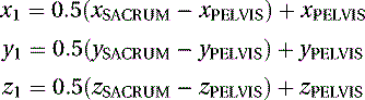
(5.30)
We then use Equation (5.19) to find the length of line segment A. This is done by assuming the system is at its base state:
(5.31)
We know the coordinates of three points in space: L1(xL1, yL1, zL1), PELVIS(xPELVIS, yPELVIS, zPELVIS), and SACRUM(xSACRUM, ySACRUM, zSACRUM). The constants (a, b, c, and d) of Equation (5.1) can be calculated by the determinants in Equations (5.2) through (5.5), which we can expand as follows:


(5.32)
(5.33)
(5.34)
(5.35)
We proceed to find the plane's normal N direction cosines (σx, σy, σz), using Equations (5.10) through (5.12).
We have a line segment B from P1 to P2 that is parallel to N and of equal length to A. We know that any two parallel lines in space have the same direction cosines, so the direction cosines of B are the same as the direction cosines of N. We use Equations (5.20) through (5.22) to obtain the location of P2: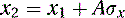
(5.36)
(5.37)
(5.38)
We know the angle α between A and B is 90°, so to obtain LUMBAR's position, we need to rotate B 90° about the local z-axis at P1. We use the following set of matrix transformations:
(5.39)
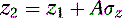
Thorax
Point THORAX is calculated by the same method as LUMBAR, using T7, LUMBAR, and L1 instead of L1, PELVIS, and SACRUM. We don't use P1 at all; instead, we use LUMBAR. The final transformation will yield point P3, which can then be transformed by the depth difference d, which can be calculated from the base position. Figure 5.3 shows the elements used to calculate THORAX.
 |
| Figure 5.3 Elements used to calculate the position of THORAX. |
Loneck
Point LONECK is calculated by the same method as THORAX, using T1, THORAX, and T7 instead of T7, LUMBAR, and L1. Figure 5.4 shows the elements used to calculate LONECK.
 |
| Figure 5.4 Elements used to calculate the position of LONECK. |
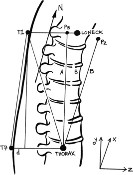
Upneck
For point UPNECK, we use the same method as for THORAX, using C1, LONECK, and T1. Figure 5.5 shows the elements used to calculate point UPNECK.
 |
| Figure 5.5 Elements used to calculate the position of UPNECK. |
Head
Point HEAD is used to help orient the joint that has its root at UPNECK. We assume that it is located between LHEAD and RHEAD. We calculate the location of this point by simply applying (5.13)(5.14)(5.15)(5.16) and (5.17). Figure 5.6 shows the calculation of point HEAD.
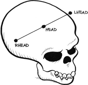 |
| Figure 5.6 The calculation of point HEAD. |
Torso
It is a good idea to separate the front part of the ribcage from the spine, as it is not as flexible, especially in the sternum area. We do this by using markers C7 and STERNUM, combined with point LONECK, as shown in Figure 5.7.
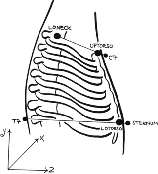 |
| Figure 5.7 Calculating the position of the torso points UPTORSO and LOTORSO. |
Point UPTORSO is simply calculated by obtaining a point in between C7 and LONECK, using (5.13)(5.14)(5.15)(5.16) and (5.17), with an appropriate value for parametric variable u that is just enough to internalize the point. A value of 0.05–0.1 will do in most cases, but it really depends on the width of the performer and the diameter of the marker.
Shoulder and Arm
Most of the motion capture data files that I have seen do not account for the three joints that form the shoulder complex: the glenohumeral joint between the humerus and the scapula, the acromioclavicular joint between the distal clavicle and the acromion, and the sternoclavicular joint between the medial clavicle and the manubrium. None of the common deformation schemes works well with shoulders, but it helps to have a somewhat anatomically correct setup. If we use an internal deformation technique, such as a muscle-based system, the correctness is imperative.
The shoulder complex will be formed by joints that go from point UPTORSO to CLAVICLE, down to SCAPULA, and back up to UPARM (see Figure 5.8).
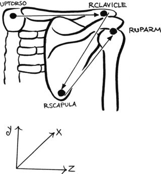 |
| Figure 5.8 The points that define the shoulder joints. |
We first calculate point CLAVICLE, using markers SHOULDER and SCAPULA, and point LONECK. Using (5.13)(5.14)(5.15)(5.16) and (5.17), calculate a point P1 between the SHOULDER marker and point LONECK. The parametric variable u should be defined so as to place P1 almost above the acromioclavicular joint. We then calculate point CLAVICLE, using the same method for a line between P1 and SCAPULA. Although it appears that the constructs of the shoulder complex are not well suited for animation, by using SCAPULA and SHOULDER to calculate the position of CLAVICLE, we are establishing links between the parts. This setup may not be optimal for keyframe animation, but it is well suited for captured motion data.
Marker SCAPULA can be used as is, because it only serves as an orientation point for CLAVICLE, but UPARM must be placed at the pivot point of the glenohumeral or shoulder joint. We do this by calculating a midpoint LOARM between markers IELBOW and EELBOW and using a line between SHOULDER and LOARM to find the location of UPARM (see Figure 5.9).
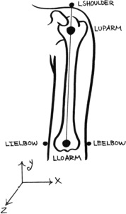 |
| Figure 5.9 The upper arm. |
To replicate as faithfully as possible the rotation of the lower arm, where the radius rotates over the ulna, we will require two bones that we can originate at point LOARM. One will be aligned to point IWRIST and the other to EWRIST. Finally, the hand rotation is obtained by aligning a midpoint P1, between IWRIST and EWRIST, to the HAND marker (see Figure 5.10).
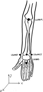 |
| Figure 5.10 The lower arm. |
Leg and Foot
The upper leg pivot point is located at the head of the femur. We trace a line between HIP and PELVIS, and place FEMUR at about 35% of the distance between the two. We then use the same line to create UPLEG, just inside the greater trochanter. Point LOLEG, located at the knee, is positioned by calculating the midpoint between markers IKNEE and EKNEE, as shown in Figure 5.11.
 |
| Figure 5.11 The upper leg. |
Point UPFOOT is obtained via a method similar to that used to calculate LUMBAR, using point LOLEG and markers HEEL and FOOT. We use marker ANKLE later to maintain orientation. LOFOOT is calculated using FOOT, TOE, and UPFOOT.
Orientation of the Bones
You now have a set of points in space where a set of local Cartesian coordinate systems will be located. These represent the roots of joints that will form the mechanical setup. The base position is assumed to be the laboratory frame in time where all these coordinate systems are in their initial state. You can further assume that the longitudinal axis of each segment is the line between the root and the target points, but the rotation about the longitudinal axis has to be locked down to a moving rigid segment, such as the ones defined in the marker setup design section in Chapter 3.
Some high-end animation programs, such as Maya, provide the ability to assign a point in space as a root and another as a target or an effector, using other points as orientation or aim constraints. If this is the case, you can now use these points, in combination with the marker sets that were defined as rigid segments in Chapter 3, to place your joints and constrain their primary orientation. If your software does not allow you to do this, you need to perform these calculations yourself, using the direction cosines described previously to calculate the angular changes in the plane and apply them to the bone. In this case, you might want to consider using a nonhierarchical system, as it would require fewer computations.
Facial Motion Capture
Preparing the Data
Applying motion capture data to a digital model is not very user friendly. Facial data is even more of an undertaking. The main issue is that there aren't many software packages that have the necessary tools as they exist for body data.
To obtain decent facial data, one must apply enough markers to the face. A good layout will have markers placed along the lines of the main facial muscles. Figure 5.12 shows a facial marker setup that follows this concept.
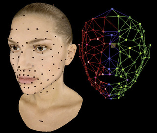 |
| Figure 5.12 Facial marker layout. Photo courtesy of Digital Concepts. |
Facial data is translational and it doesn't matter if the face is captured with the performer sitting still or moving; the data still needs to be stabilized before applying it to a digital character in order to remove any head motion from it. That process can be done by capturing the head motions and globally subtracting them from each of the markers that cover the face. It can be done in animation software or in packages such as Matlab.
An interesting software package that is used to manipulate motion data is Vicon Blade. Digital Concepts Group, a company founded by DJ Hauck and Steven Ilous, has created a toolset for Blade that greatly aids in the preparation of facial data, specifically in the labeling of markers, stabilization, cleanup, and retargeting. Figure 5.13 shows a screenshot of the DCG toolset.
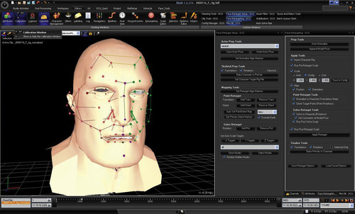 |
| Figure 5.13 The DCG toolset. Photo courtesy of Digital Concepts Group. |
Facial Character Setup
The two most widely used computer facial animation systems are the ones based on premodeled shape interpolation and the ones based on cluster or lattice deformations. Most of the facial systems today are a combination of both.
The state of the art in facial animation software is a muscle system combined with shape interpolation. This kind of system is not widely used because of the lack of available commercial technology as most of the currently existing systems are proprietary.
Once the data has been prepared as described in the previous section, it should be imported into the animation software where the character setup will be created.
Assuming a model with a body rig already exists, that data should be placed globally under the last node that pertains to the head motions. The data also should be offset globally to match as best as possible with the digital model's face. If the data was retargeted properly, it should be an easy match.
The data can then be used to drive a series of joints that will ultimately be used to deform the face. I particularly like to avoid the joints and drive a control mesh by constraining all its vertices directly to the data. I call this “The Mug” (Figure 5.14).
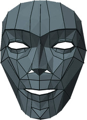 |
| Figure 5.14 The Mug. |
The mug can be used as one of many layers of controls that could be used to animate a face. It would deform the face using a deformer that allows a piece of geometry to ride on another. An example of a deformer such as this would be the Maya muscle.
By designing the rig in layers, an experienced setup artist can add different controls and deformers in modular ways, allowing the face to be animated by many possible methods such as blendshapes, manipulating muscles, and retargeted facial motion data.
Shapes can also be driven by motion data. This is very useful, especially if the character doesn't have facial features that resemble a human. For every blend shape, there would be a corresponding human expression. I call this group of human expressions the “training set.” The final blend of shapes would be calculated frame by frame by an algorithm that would study the expression in the human data and calculate the blend in the training set that would achieve best the frame's expression. That blend could be applied to the nonhuman shapes, obtaining the corresponding final expression.
The facial systems that were used to create Beowulf and Avatar follow this principle. The shapes they use are based on the Facial Action Coding System list of expressions created by Paul Eckman. Obviously, the more shapes are used, the better will be the resulting expression.
The algorithm used to find the shape combination would analyze the options and calculate the final recipe. Mathematically, this would be considered an Inverse Problem, which is loosely defined as a problem where the answer is known but not the question. We know what the final expression looks like but we don't know what combination was used to create it. This kind of inverse problem would be solved by using a geometric fitting algorithm such as least squares or nonlinear regression. These methods are readily available in software packages such as Matlab.
Tips and Tricks
Switching the Order of Rotations
There are cases in which your data will be delivered based on a predefined order of rotations with which your software may not be compatible. If this is the case, you will have to recompute your data to reflect an acceptable order. Most of the common captured motion data files contain rotations specified in Euler angles. We will combine all the rotations into one matrix and then decompose it in a way that will yield the desired order of rotations.
The 3 × 3 rotation matrix of θ about the x-axis is given by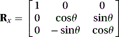
(5.40)
The 3 × 3 rotation matrix of ϕ about the y-axis is given by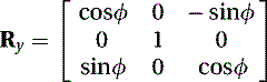
(5.41)
The 3 × 3 rotation matrix of ψ about the z-axis is given by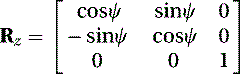
(5.42)
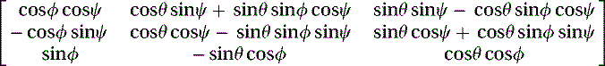
We begin by creating the matrix that will contain all the rotations. If the data file contains rotations in the XYZ order, we would multiply the matrices in the proper order as follows: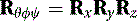 where θ = rotation about the x-axis, ϕ = rotation about the y-axis, and ψ = rotation about the z-axis. We obtain the following matrix:
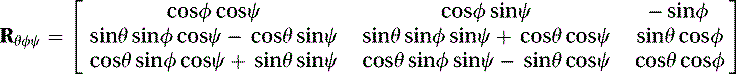
(5.43)
(5.44)
Because we know all the values of θ, ϕ, and ψ, we can solve the equations and represent the matrix as follows: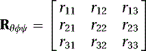
(5.45)
We next build the matrix that we will use to extract the new order of rotations. If we had to convert the order of rotations to ZYX, for example, we would multiply the matrices in (5.40)(5.41) and (5.42) as follows: where after decomposing, θ = rotation about the z-axis, ϕ = rotation about the y-axis, and ψ = rotation about the x-axis. We obtain the following equation:
(5.46)
(5.47)
We simplify the equations by multiplying both sides by  , which is equal to
 obtaining
(5.48)
(5.49)
From Equation (5.49), we can extract
(5.50)
We finally obtain the value of ψ by the following: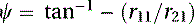
(5.53)
Having ψ, we can calculate the value of θ using Equation (5.49):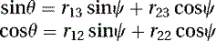 which can be used to compute θ:
(5.54)
(5.55)
Finally, we assign the following values: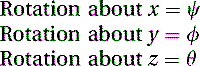
(5.58)
Distribution of Rotations
About the Longitudinal Axis
Some of the most common deformation systems do not yield great results when a joint or a bone rotates about its longitudinal axis. The lower arm is almost always a problem area in this respect.
If your character setup does not provide a mechanical solution for pronation and supination as specified in the character setup section, chances are that the longitudinal rotations of the lower arm are attributed to the wrist. An alternative to redesigning the skeletal structure is to distribute the wrist rotations equally between the wrist and the elbow. Better yet, distribute the total longitudinal rotations of the arm among the wrist, elbow, and shoulder joints. This is a very easy process, provided that the rotation along the longitudinal axis is the last transformation, which should be standard practice in any character setup.
When using captured motion data from a hierarchical rotational file, assuming that the longitudinal axis is y and that the rotation order is ZXY or XZY, you could simply solve the problem with a set of expressions as follows: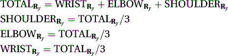
(5.59)
You can distribute the rotations in different ways, perhaps applying less to the shoulder.
With Shifting Pivot Point
Another interesting idea is to distribute rotations between joints in a way similar to the actual rotations of the spine, where a single vertebra has a maximum possible range of rotation. The rotation starts with the lowermost vertebra and continues until its maximum range has been reached. At that point, the rotation and the pivot point carry over to the next vertebra until it meets its maximum, and so on (see Figure 5.15). For example, if a vertebra has a range of rotation of 10° for a given axis, rotating the whole spine 36° would result in the rotation of the lowermost four vertebrae: the first three by 10° and a fourth by 6°. This method does not yield the same result as rotating the lowest vertebra in the spine by 35° along its single pivot point, but it is close to half, or 18°. Of course, this is dependent on the separation between vertebrae, which needs to be uniform.
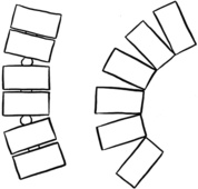 |
| Figure 5.15 Distributed rotations with shifting pivot point. |
The following pseudocode converts a single rotation group into a set of three distributed rotation groups with shifting pivot point. It assumes the rotations are stored in rx, ry, and rz, respectively; that y is the longitudinal axis; and that the rotation order is XYZ.
/* Declare various variables */
int num_joints = 3;/* Number of joints */
float rot_vector[3];/* Incoming rotations*/
float rot_residual[3];/* Carry over rotations */
float rot_joint_vector[num_joints][3];/* Outgoing rotations*/
float rot_joint_limit; /* Maximum rot per joint */
int i; /* Loop variable */
/* Write incoming rotations into array */
/* Double rx and rz to approximate result to single pivot */
rot_vector[0] = rx * 2;
rot_vector[1] = ry;
rot_vector[2] = rz * 2;
/* Set rotation limit per joint */
rot_joint_limit = 15;
/* Initialize residual array */
/* For longitudinal axis divide rotations equally */
rot_residual[0] = rot_vector[0];
rot_residual[1] = rot_vector[1] / num_joints;
rot_residual[2] = rot_vector[2];
/* Start processing rx */
/* If rx is greater than the limit, start distribution */
if (abs(rot_vector[0]) ] rot_joint_limit) {
i = 0;
/* Start the distribution loop */
/* Check if there is carry over and additional joints */
while (abs(rot_residual[0]) ] 0 && i [ num_joints) {
/* If rotations are positive */
if (rot_vector[0] ] 0) {
/* If the rotation left over is less than limit */
/* apply it all to current joint*/
if (abs(rot_residual[0]) [ rot_joint_limit)
rot_joint_vector[i][0] += rot_residual[0];
/* Otherwise, apply limit to current joint*/
else
rot_joint_vector[i][0] += rot_joint_limit;
/* If joint is over limit, save extra in residual */
if (rot_joint_vector[i][0] ] rot_joint_limit) {
rot_residual[0] += rot_joint_vector[i][0] –
rot_joint_limit;
rot_joint_vector[i][0] = rot_joint_limit;
}
/* Subtract current rotation from new residual */
rot_residual[0] -= rot_joint_limit;
/* Make sure residual isn't negative */
if (rot_residual[0] [ 0)
rot_residual[0] = 0;
}
/* Process negative rotations */
else {
/* If the rotation left over is less than limit */
/* apply it all to current joint*/
if (abs(rot_residual[0]) [ rot_joint_limit)
rot_joint_vector[i][0] += rot_residual[0];
/* Otherwise, apply limit to current joint*/
else
rot_joint_vector[i][0] -= rot_joint_limit;
/* If joint is over limit, save extra in residual */
if (abs(rot_joint_vector[i][0]) ] rot_joint_limit) {
rot_residual[0] -= (rot_joint_vector[i][0] –
rot_joint_limit);
rot_joint_vector[i][0] = -rot_joint_limit;
}
/* Subtract current rotation from new residual */
rot_residual[0] += rot_joint_limit;
/* Make sure residual isn't positive */
if (rot_residual[0] ] 0)
rot_residual[0] = 0;
}
i++;
/* End of loop */
}
}
/* If rx is smaller than the limit, apply all to first joint */
else {
rot_residual[0] = 0;
rot_joint_vector[0][0] = rot_vector[0];
}
/* Process ry (longitudinal axis) */
i = 0;
while (i [ num_joints) {
/* Rotate joint */
rot_joint_vector[i][1] = rot_residual[1];
i++;
}
/* Start processing rz */
/* If rz is greater than the limit, start distribution */
if (abs(rot_vector[2]) ] rot_joint_limit) {
i = 0;
/* Start the distribution loop */
/* Check if there is carry over and additional joints */
while (abs(rot_residual[2]) ] 0 && i [ num_joints) {
/* If rotations are positive */
if (rot_vector[2] ] 0) {
/* If the rotation left over is less than limit */
/* apply it all to current joint*/
if (abs(rot_residual[2]) [ rot_joint_limit)
rot_joint_vector[i][2] += rot_residual[2];
/* Otherwise, apply limit to current joint*/
else
rot_joint_vector[i][2] += rot_joint_limit;
/* If joint is over limit, save extra in residual */
if (rot_joint_vector[i][2] ] rot_joint_limit) {
rot_residual[2] += rot_joint_vector[i][2] –
rot_joint_limit;
rot_joint_vector[i][2] = rot_joint_limit;
}
/* Subtract current rotation from new residual */
rot_residual[2] -= rot_joint_limit;
/* Make sure residual isn't negative */
if (rot_residual[2] [ 0)
rot_residual[2] = 0;
}
/* Process negative rotations */
else {
/* If the rotation left over is less than limit */
/* apply it all to current joint*/
if (abs(rot_residual[2]) [ rot_joint_limit)
rot_joint_vector[i][2] += rot_residual[2];
/* Otherwise, apply limit to current joint*/
else
rot_joint_vector[i][2] -= rot_joint_limit;
/* If joint is over limit, save extra in residual */
if (abs(rot_joint_vector[i][2]) ] rot_joint_limit) {
rot_residual[2] -= (rot_joint_vector[i][2] –
rot_joint_limit);
rot_joint_vector[i][2] = -rot_joint_limit;
}
/* Subtract current rotation from new residual */
rot_residual[2] += rot_joint_limit;
/* Make sure residual isn't positive */
if (rot_residual[2] ] 0)
rot_residual[2] = 0;
}
i++;
/* End of loop */
}
}
/* If rz is smaller than the limit, apply all to first joint */
else {
rot_residual[2] = 0;
rot_joint_vector[0][2] = rot_vector[2];
}
/* Apply new values to all joints */
Using Parametric Cubic Curves
Other methods for creating smoother relationships between joints involve the generation of curves, using markers or calculated points as control points. A parametric cubic curve can be generated using two or four points. To produce a parametric cubic curve using two points, use the following three polynomials of the third order: where u is the parametric variable that has an interval from 0 to 1. u = 0 represents the first point, and u = 1 represents the second point. Any value in between can be used to calculate additional points as needed.
(5.60)
The slope of the curve is given by the two tangent vectors located at the ends of the curve. The components of each tangent vector are given by differentiating Equation (5.60) as follows: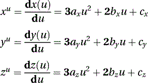
(5.61)
By solving the equations using u = 0 and u = 1 where the two points are known, you can obtain the values of the coefficients (a, b, c, and d) and then proceed to calculate intermediate points.
When linking two point segments, such as in the vertebral column, make sure that the tangent vectors at the ends of the curves are matching, thus resulting in a single smooth curvature.
Interpolation
There are many instances when you will need to interpolate rotations between different captured motion data files. Common cases are the blending or stitching of different motions or creating a looping motion for actions like walking or running.
As I've stated in previous chapters, the success of blending or looping depends a great deal on the compatibility of the motion data. The points where the data files are to be blended need to be similar in their pose and have a similar timing of motion. If this is true, half the work is already done.
Quaternions
Rotations in captured motion data files are usually represented by Euler angles combined with a predefined order of rotations. This is not the best format to use when interpolating between two rotations because in order to reach the final orientation, three ordered rotations about separate axes have to occur. There are 12 combinations by which the final orientation can be reached, resulting in different representations of the 3 × 3 rotation matrix. Furthermore, Euler angles have the problem commonly known as gimbal lock, whereby a degree of freedom is lost due to parametric singularity. This happens when two axes become aligned, resulting in the loss of the ability to rotate about one of them.
Interpolating translations using Cartesian coordinates works mainly because translations are commutative, which means that to arrive at a certain location in space the order of translations is not important; thus, there are no dependencies between the transformations. Rotations represented by Euler angles are noncommutative, which means that their order cannot be changed and still yield the same final orientation. It also means that the transformations depend on each other.
Interpolation between orientations is best done by using quaternions, which, as their name implies (from Latin), are sets of four numbers, one of which represents a scalar part and three that represent a vector part. A quaternion q can be represented by the following equation: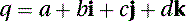 where the coefficients a, b, c, and d are real numbers, and i, j, and k are the axes. As in complex numbers of the form
 where i2 = −1, for quaternions, each of i2, j2, and k2 are also equal to −1. Thus, quaternions are extensions of complex numbers that satisfy the following identities:
(5.62)
(5.63)
(5.64)
The condensed notation for a quaternion is where s is the scalar part and v is the vector part, so that
(5.65)
(5.66)
Quaternion multiplication can be expressed as follows:
(5.67)
Quaternion multiplication is noncommutative, so q1q2 is not the same as q2q1. The magnitude of a quaternion can be determined by the following equation: where
where  is the conjugate of the quaternion, defined as
(5.68)
(5.69)
A unit quaternion has a magnitude of 1, so from Equation (5.68) we can determine that where q is a unit quaternion. Unit quaternions are used to represent rotations and can be portrayed as a sphere of radius equal to one unit. The vector originates at the sphere's center, and all the rotations occur along its surface. Interpolating using quaternions guarantees that all intermediate orientations will also fall along the surface of the sphere. For a unit quaternion, it is given that
(5.70)
(5.71)
The inverse of a quaternion is defined as but for a unit quaternion it can be reduced to
(5.72)
(5.73)
A unit vector p can be represented in quaternion notation as one without a scalar part, also called a pure quaternion:
(5.74)
The rotation of p can be computed by the following equation: where P′ is also a pure quaternion. This rotation can also be achieved by applying the following matrix:
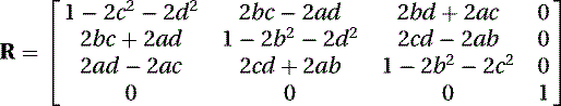
(5.75)
(5.76)
Before we start looking at the interpolation process, we need to establish that a rotation of θ about a unit vector p can be performed by using the following unit quaternion: which means that separate rotations about the x, y, and z axes can be represented as
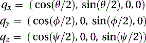 respectively. We can now convert our Euler angles from the captured motion data file into quaternion space by simply multiplying the quaternions in the proper order. For example, a rotation in XYZ order would be given by using Equation (5.67) to perform the following multiplication:
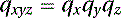
(5.77)
(5.78)
(5.79)
Converting a rotation matrix to a quaternion is a simple process. Let us assume we have a 4 × 4 transformation matrix of the form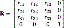
(5.80)
We obtain the trace, which is the sum of its diagonal elements r11, r22, and r33 so that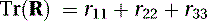
(5.81)
To find the converted quaternion q(W, X, Y, Z), we start by finding the value of the scalar W using Equation (5.81):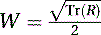
(5.82)
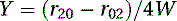
The vector elements are calculated as follows: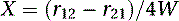

(5.83)
(5.84)
(5.85)
Once we are in quaternion space, we can proceed with the interpolation. The most commonly used interpolation method for quaternions is called spherical linear interpolation, or slerp. Because of its spherical nature, this method guarantees that any intermediate quaternions will also be unit quaternions. Slerp computes the angle θ between both quaternions as vectors in two-dimensional space, using their scalar product. If we have two quaternions q1 and q2, we can find θ as follows: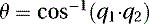
(5.86)
To calculate quaternion q′ in between q1 and q2 using slerp, we use a parametric variable u with interval from 0 to 1 and the following equation:
(5.87)
If θ is equal to 0, the slerp will run into computational problems due to division by zero. If this is the case, instead of using slerp, we just use linear interpolation. Other problems with slerp occur when θ is equal to multiples of π/2. Those problems can be avoided by changing either one of q1 or q2 to an approximation. For example, we can use q2 and q3, an adjacent keyframe, to generate a third quaternion q4 that is as close to q2 as possible without falling in the problem area; then we could proceed with the original interpolation using q1 and q4 instead of q1 and q2.
We now must convert q′ (W, X, Y, Z) back into a rotation matrix R of the form shown in Equation (5.80). We use the matrix in Equation (5.76), which now becomes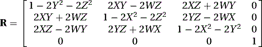
(5.88)
We can finally decompose R into Euler angles if we need to using the method explained in the section “Switching the Order of Rotations.”
Keyframe Reduction
In some situations, you may want to reduce the number of keyframes in your data. This is not the same as downsampling, as you will keep the same sampling rate or frames per second at which the data is supposed to play back. Depending on what the purpose is, you may be able to reduce the number of keyframes automatically, but for the highest quality you may have to do it manually.
Removing every nth keyframe is not a good method because it doesn't take into account the ratio of change from one keyframe to the next. The preferred method is to find areas in your curve that are smooth and don't fluctuate too much, and then delete all keyframes that fall within two predetermined boundary keyframes. This is a long process if you have a character with dozens of joints, but you can accelerate it by using an algorithm that looks for differences in the curves.
There are many commercial software solutions that allow you to perform several types of fitting to your curves. Many load your data into a spreadsheet where you can perform a variety of manual or automatic operations, including smoothing and other noise reduction methods. A good method for curve fitting is the least squares method, which most software packages support. Matlab is probably the most popular software package that can be used to do all kinds of curve analysis and manipulations.
..................Content has been hidden....................
You can't read the all page of ebook, please click here login for view all page.