
We just said it before, and we’ll say it again: you probably won’t ever use the intersection operator, for reasons we’re about to detail. But the operator is available, just the same; and what the operator – signified by the @ sign – does, for what it’s worth, is reduce a dynamic array spilled range to a single-celled output, thus emulating the behavior of formulas in pre-Excel 365 versions.
An example: you’ll recall our Beatles range a couple of hundred pages ago cataloging the names of the erstwhile Fab Four. In Excel 365, entering =Beatles will of course spill the names down the column in which the range name was entered. But in Chapter 2 we pointed out that imitating that action in a pre-365 iteration would, by default, only return the first entry in the range, issuing under the sway of what’s called implicit intersection. As described in that chapter, the only, limited, means for returning all four names would have required the user to select four destination cells at the outset that parallel the projected output of four names, click in the Formula Bar, write =Beatles there, and put the finishing touch on the process by tapping out the storied Ctrl-Shift-Enter sequence, kind of a spreadsheet chord. But since you’d need to select the four cells before you proceed, that technique isn’t quite of the dynamic array variety.

A screenshot of an excel sheet. It has 3 rows and 4 columns. The entries are as follows; Row 1: 1, 4, 4, and equals a 1: a 3 asterisk b 1: b 3, row 2: 2 and 5, and row 3: 3 and 6.
Output shortfall: a pre-dynamic array multi-cell multiplication
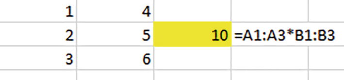
A screenshot of an excel sheet. It has 3 rows and 4 columns. The entries are as follows; Row 1: 1, and 4, row 2: 2, 5, 10, and a 1: a 3 asterisk b 1: b 3 and row 3: 3 and 6.
Same formula, different result
Now if you deem that result something of a curiosity, writing the same formula in C2, one cell down, would yield
Moreover, even if you were to finalize these formulas with none other than the iconic Ctrl-Shift-Enter, they’d still evaluate to a single-celled result.
And for good measure if you were to write the selfsame formula in say, D12, you’d unleash a #VALUE! error message upon the cell.
All these quirky outcomes hinted at the workings of implicit intersection, which, you’ll be happy to know, has been consigned to the past tense. Because pre-365 formulas weren’t directly capable of outputting multiple results to cells, even when they attempted to, they were forced to decide which single result they would be able to return. And in formulas such as the ones you see above that result was lined up – literally – with the row on which the formula sat, explaining in turn why a formula entered in D12 would provoke an error message – because row 12 in the worksheet doesn’t line up with any of the rows 1 through 3, where the data were positioned. That’s implicit intersection – in which the formula is forced to intersect only with the value sharing its row (or column, if the formula were written on the same column as the value).
But again, of course, virtually none of this matters now. Dynamic array formulas routinely release their spill range of values down or across, or down and across, as many cells as they require, and the formulas can be written anywhere in the worksheet besides.
=(@A1:A3*@B1:B3)

A screenshot of an excel sheet. It has 3 rows and 4 columns. The entries are as follows: Row 1: 1, 4, 4, and equals left parenthesis at the rate a 1: a 3 asterisk b 1: b 3 right parenthesis, row 2: 2 and 5, and row 3: 3 and 6.
Holding back; this dynamic array formula yields one result

A screenshot of an excel sheet. It has 3 rows and 3 columns. The entries are as follows: Row 1: 1 and 4, row 2: 2, 5, 10, and equals left parenthesis at the rate a 1: a 3 asterisk b 1: b 3 right parenthesis, and row 3: 3 and 6.
A comedown: once again, the formula only references the value on its row
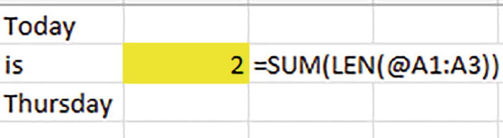
A screenshot of an excel sheet. It has 3 rows and 3 columns. The entries are as follows: Row 1: today, row 2: is, 2, and equals sum left parenthesis l e n left parenthesis at the rate a 1: a 3 right parenthesis, right parenthesis and row 3: thursday.
Going to great length: implicit intersection again forces one result
And those results mimic what you’d see in a pre-365 edition of Excel.
All of which inspires the obvious question: when would I need to use this? The short answer: probably never.
After all, the likelihood you’d actually reach back for a feature that Excel has decided to overrule takes retro nostalgia a step too far. Several web-based discussions of the operator that I’ve seen suggest uses for the function that seem forced and contrived, as if their authors are similarly puzzled by the whole idea.
But in the interests of giving Microsoft the benefit of the doubt, allow me to spin a halfway plausible narrative in which the implicit intersection operator might be of service.
Where You Might Use the Intersect Operator – Maybe
=SUM(LEN(A1:A3))
can be written by all of the students, Excel version notwithstanding – provided of course that the pre-365 users bang out Ctrl-Shift-Enter to complete the formula.
But another contingency looms: what if a pre-365 user writes an array formula and forgets to strike Ctrl-Shift-Enter, pressing Enter instead – a mistake most easily committed?
What happens of course is implicit intersection. Write =SUM(LEN(A1:A3)) in a pre-365 version, tap Enter alone, and you get one value – not the sum of the lengths of the three words introduced in A1:A3, but again, the length of the word on the row in which you’ve composed the formula.
But remember you, the teacher, have Excel 365 under your hood, and so you can’t recreate what’s happening – because Excel 365 has eliminated implicit intersection.
=SUM(LEN(@A1:A3))
Enter that expression and your formula will likewise return but one value. And as a consequence, you’ll be able to confirm – and show – to the pre-365 user what result she’ll see.
Thus, recourse to the implicit intersection operator in Excel 365 could serve a meaningful instructional purpose. But if teaching isn’t your bag, the @ sign isn’t where it’s at.
They’re Here, Probably: The Newest Dynamic Array Functions
But now we’re going to begin to take a concerted look at some other functions that you probably will use – once you determine that they’re there.
They’re the newest batch of dynamic array functions – 14 in toto – that for the most part offer Excel users a number of enhancements to their customary ways of doing their work. Instead of dealing out an assortment of new means for number crunching, the new functions by and large issue a set of novel and important tools for organizing, and reorganizing, your datasets in ways that facilitate the crunching; and if that description is long on abstractions and short on examples, the examples will emerge in the ensuing chapters.
And yes, you should have the new functions now, pursuant to Microsoft’s announcement on September 29, 2022 that “These functions are now fully deployed to Excel for the Web and users of Office 365 on the Current Channel”.

A screenshot of an excel sheet. It has 8 rows and columns. The entry for 1st row and 3rd column is equals c h o. Below it is a summation tool with 3 options f x choose, f x choose columns, and f x choose rows.
Where did THEY come from?: CHOOSECOLS and CHOOSEROWS, two of the new dynamic array functions
TEXT SPLIT
TEXT BEFORE
TEXTAFTER
TOCOL
TOROW
WRAPSOL
WRAPROWS
VSTACK
HSTACK
CHOOSECOLS
CHOOSEROWS
TAKE
DROP
EXPAND
can in fact be understood as a smaller set of groupings, because some address the organization of rows in a dataset, while others perform similar work on columns, and the like. And that means that acquainting yourself with the new set won’t take quite so long as you may first assume – or fear.
Chapter 10 will kick off our review of the new functions by investigating the three that are designed to address – and solve – a batch of classic spreadsheet problems besetting the handling of text – TEXT SPLIT, TEXT BEFORE, and TEXT AFTER.