
Coming to a Hard Drive Near You
The three new dynamic array text functions take collective aim at a class of age-old and related spreadsheet problems – namely, how to separate, or parse, a cell containing a text string into its constituent words.
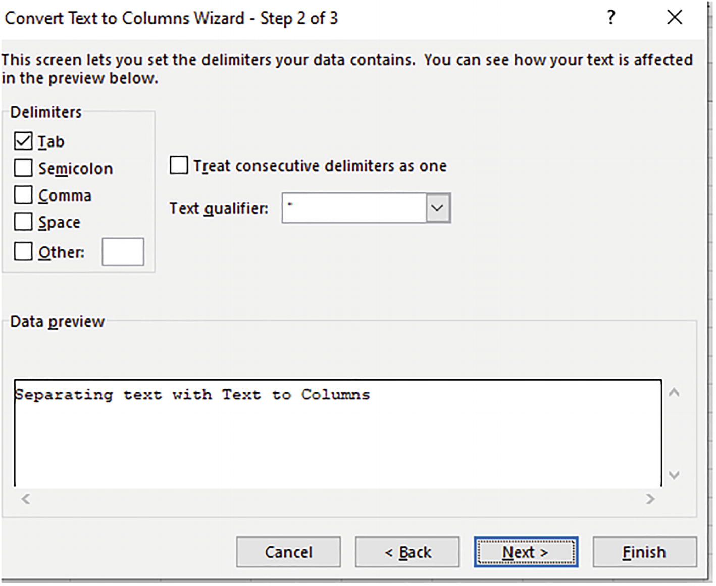
A screenshot of a tab titled convert text to columns wizard - step 2 of 3. Among the checkboxes for tab, semicolons, comma, space, and other the one for tab is ticked. The field entry for data preview reads separating text with text to columns.
Microsoft’s words – assigning each word to a cell via Text to Columns
Text to Columns works principally by enabling the user to define a delimiter, or delimiters, by which the text could be demarcated into a one-word-per-column motif. In the above shot the user would tick the “space” box, the character which would delimit the text into its respective words wherever it happened upon a space in the text entry.

A screenshot of a header row in a spreadsheet. The separated field names are lottery number, project name, P H N, street name, boro, N C slash pres, oversight, and agency.
The great divide: a header row in CSV format before its field names have been separated
Remember that all those budding headers (far more than you’re actually viewing above) are jammed into a single cell, and Text to Columns would seize upon the delimiting commas and carve out a discrete a field name for each and every term hemmed in by those commas, and then proceed to do the same for all the comma-ridden rows beneath the headers as well, converting them all into field data.
Text to Columns has put in years of honorable service, but because it’s click-based, its flexibility is stunted. For example, if I wanted to separate and sort the data – say, comma-separated test scores – Text to Columns would only perform the separation, but not the sort. Or if I needed to disentangle comma-separated values and then stack them vertically, again, you’d need to look elsewhere – in the direction of formulas.
And indeed – a number of formulaic means for parsing, or extracting, words or segments of text have long been made available, and we’ve already viewed some of them, for example, MID, LEFT, and SEARCH. But as this (https://www.linkedin.com/posts/andrewcharlesmoss_extracting-and-splitting-text-activity-6928128981799997440-NGpl/?utm_source=linkedin_share&utm_medium=member_desktop_web) piece notes, those strategies can get rather convoluted, and can stymie the user who’s up against that quintessential text roadblock – separating first, middle, and last names that are all huddled in the same cell.
But help has arrived – in the form of three new, streamlining formulas that go a long way toward smoothing the bumps pockmarking the road to successful text separation – TEXTSPLIT, TEXTBEFORE, AND TEXTAFTER.
TEXTSPLIT: Piecing It Together
=TEXTSPLIT(text,column delimiter,row delimiter,ignore empty,match mode,pad width)
As we’ll see, the first two arguments – the one requiring you to identify the text you want to split and the one that names the delimiter(s) – are essential, while the remaining four offer themselves as options.
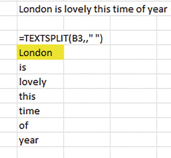
=TEXTSPLIT(B3," ")

A cropped screenshot of a spreadsheet. The words in each cell under the formula text split read, London, is, lovely, this, time, of, and year. The cell with London in it is highlighted.
Spaced out: each word is assigned its own cell
Here TEXTSPLIT searches our phrase for every space, the character we’ve nominated as the column delimiter. Each textual instance preceding a space is allotted its own cell, and as a result every word is properly separated, or split.
=TEXTSPLIT(B3,," ")
A cropped screenshot of a spreadsheet. The words are arranged in a columnar manner under the formula. The texts in the column read: London, is, lovely, this, time, of, and year. The cell with London in it is highlighted.
London’s text is falling down: TEXTSPLIT generates a vertical word split
We’ve seen something like this before, for example, in our survey of the SEQUENCE function. The formula’s additional comma bypasses the column delimiter argument and actuates a row delimiter instead – the space again, but which now acts as a kind of de facto line break, wrapping the split items down a column.
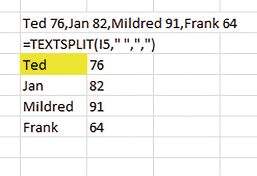
Ted 76,Jan 82,Mildred 91,Frank 64
=TEXTSPLIT(I5," ",",")

A cropped screenshot of a spreadsheet. The given text is split into 2 columns under the formula text split. The row entries are Ted, 76; Jan, 82; Mildred, 91; and Frank, 64. The cell with Ted in it is highlighted.
Every which way; the text is split both across and down a column
The space delimiter spills each student name/score downwards, while at the same time the comma neatly pairs each name and its corresponding score horizontally. Just remember to line up all those quotation marks properly.
The test scores returned above by TEXTSPLIT nevertheless have the status of text (note their left alignment). There are ways of treating these as numeric values, though, for example, through the VALUE function.
=SORT(TEXTSPLIT(I5," ",","),2,-1)
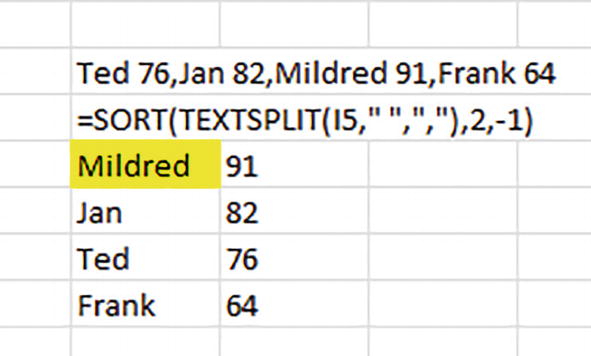
A cropped screenshot of a spreadsheet. The text is divided into 2 columns under the sort formula. The row entries are Mildred, 91; Jan, 82; Ted, 76; and Frank, 64. The cell with Mildred in it is highlighted.
Sorting the scoring in a single cell
(Note again that Excel allows the sort to proceed, even though the scores are officially text-formatted.)
There’ll be more to be said about TEXTSPLIT’s coupling of column and row delimiters a bit later.
Choose Your Delimiters
But who insisted that the space character serve as TEXTSPLIT’s only delimiter? No one, in fact. The reality is that you can invest any character – or characters – with delimiter status.
For example, observe this phrase:
We wanted to go out, but it was raining. What was Plan B?

A screenshot of a row of a spreadsheet. The words in each cell read as follows. We, wanted, to, go, out, but, it, was, raining, what, was, plan, and B?
Spreadsheet grammar – unwanted punctuation
But we want to authorize all the above characters – period, comma, question mark, and space – to delimit words, rather than loiter idly among them, as they do in the screen shot. How do we do that?
=TEXTSPLIT(E8,{" ",",",".","?"},,1)
Got that? Still squinting, or have you given up? If so, sit back and consider this explanation: first, all the designated delimiters are bounded by a familiar pair of user-typed array-formula brackets. And inside, each delimiter is in turn enclosed by quotes and detached from the next delimiter by a comma – remembering at the same time that one of the delimiters itself is a comma, and is thus sandwiched between two of the quotes.
Is all that syntax hard to read and user-friendly? Yes and no. Of course, it works, once you coordinate all those quotes and commas; but there’s a more lucid equivalent out there about which you want to know.

A cropped screenshot of a spreadsheet column with a dropdown button. The third, fourth, and fifth-row entries are a period mark, a comma, and a question mark, respectively.
Delimiters, quote-free. The invisible space delimiter occupies the first table cell.
=TEXTSPLIT(E8,Table1,,1)
The Table1 reference serves as a proxy for the bracketed, quote-thickened delimiters, and performs in precisely the same way. Moreover, if it turns out that you need more delimiters or remember ones you’d omitted, simply enter them down the table column, and they too will automatically split any words. It’s a rather cool, far neater substitute for the official, by-the-book, bracketed delimiter argument.
You Won’t Always Ignore “Ignore Empty”
But if you travel the table route mapped above, you’ll need to make sure that TEXTSPLIT’s fourth, optional “ignore empty” argument finds a place in the formula, as we see it represented above by the 1. “Ignore empty” instructs the function to disregard a delimiter that’s unaccompanied by any text to be split – and if you overlook it, the formula we’ve detailed will inflict unnecessary spaces upon the results. For example, without “ignore empty,” the space following the word “out,” will populate a cell all its own – because the comma alongside “out” will have already delimited that word, and the space will then be treated as an empty delimiter.

A partial screenshot of a spreadsheet. The given text is split into two columns under the text split formula except for Ted. Ted and his score of 76 have a blank cell in between them. The cell with Ted in it is highlighted.
Outer space – Ted is separated from his test score by two spaces
We see that by default, superfluous delimiters are not ignored, and as such the result above makes room for both of Ted’s spaces – the first delimiting nothing, the second, the 76. And because that surplus space – which is, after all, a column delimiter – pushes Ted’s score into a new, extra, third column; that column is now imposed upon the other names, too, forcing them to emit a #N/A error message. You can’t earmark a new column for only one row, after all; it’s an all-or-nothing proposition. Ted’s row can’t receive three columns even as the other names hold to the original two.
=TEXTSPLIT(I5," ",",",1)
where the “1” issues an “ignore empty cells” order, the results return to a two-columned, error-free outcome.
Wrapping the TRIM function around formulas will eliminate superfluous spaces from a text string.
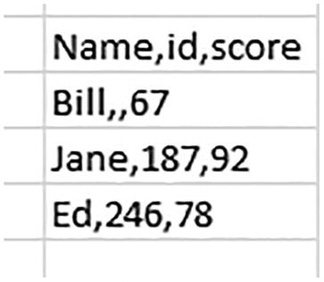
A screenshot of a spreadsheet column. The first row reads name, id, and score. The following rows list 3 names and scores, but I ds only for two, namely, Jane and Ed. The I d for Bill is not entered.
Where’s your ID, Bill?

A screenshot of 3 spreadsheet columns. The headers are name, I d, and score. The name and score columns are filled for 3 rows. The row entry for Bill's I d is blank.
These fields are lined up
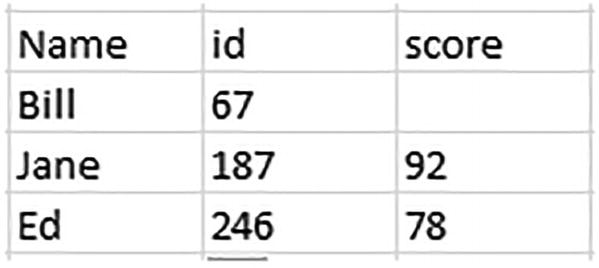
A screenshot of 3 spreadsheet columns. The headers are name, I d, and score. The name and I d columns are filled for 3 rows. The row entry for Bill's score is blank.
These fields aren’t
We see that if you do ignore the empty delimiter via the 1 argument, TEXTSPLIT will throw Bill’s next-available bit of data – 67, a test score – into the next available column, id; and as you see, that decision misaligns the data from their appropriate columns. Thus, we see that the first of Bill’s two consecutive commas supplies a placeholder for a field – id – for which information is missing. (We’ll have more to say about this example, too.)
TodayXisXThursday
=TEXTSPLIT(G12,"x")
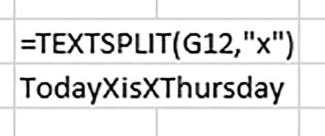
A screenshot of 2 spreadsheet rows. The formula in the first row reads text split left parenthesis G 12, double quotation x double quotation right parenthesis. The text in the next row reads today X is X Thursday.
Curious case: no change
=TEXTSPLIT(G12,"x",,,1)
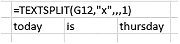
A cropped screenshot of spreadsheet cells. The formula in the first row reads text split left parenthesis G 12, double quotation x double quotation, triple comma, 1 right parenthesis. The texts in the 3 cells below it are today, is, and Thursday.
x marks the split: the text is split by TEXTSPLIT
Launching “Pad With”: A New Kind of Argument

A cropped screenshot of a spreadsheet. The given numbers and texts are split into 2 columns below the formula except for Ted. Ted and the corresponding number 76 have a blank cell in between them. The cell with Ted in it is highlighted.
Scouring pad: the “pad with” option cleans up error messages.
One could ask why Excel felt the need to coin the term “pad width,” one that doesn’t appear in any of the pre-dynamic array functions. After all, other functions, for example, XLOOKUP and FILTER, offer “if not found” or “if empty” arguments that also allow the user to post a replacement caption for formulas that would otherwise succumb to error messages. But isn’t that what “pad with” does, too? And if so, why did the folks at Microsoft’s usability team need to mint a new term for this feature that seems to do much the same as its predecessors?
The answer is that Excel could have fallen back on an existing term such as “if not found” here, but “pad with” makes a statement about the different kind of work that some of the new dynamic array functions perform. When a user performs a query with FILTER, for example, the number of results churned out by the formula will vary, depending on the filter criteria the user employs; but functions such as TEXTSPLIT and, as we’ll see, WRAPCOLS and EXPAND, ask the user to frame a spill range of fixed size at the outset, for example, three rows by four columns; and because some of those cells may, for whatever reason, be blank, the user is granted the option to fill out – or pad – the bare cells with a caption.
TEXTSPLIT and the One-Celled Dataset
A cropped screenshot of a spreadsheet. The given text and numbers are split into 2 columns below the formula. The row entries are Ted, 76; Jan, 82; Mildred, 91; and Frank, 64. The cell with Ted in it is highlighted.
Look familiar? TEXTSPLIT test splits
But now let’s flip the matter on its head. We’ve seen that TEXTSPLIT can unpack a collection of data concentrated in one cell, and distribute, or split, them into multiple, usable cells. With that skill in tow, why can’t we take existing data, repack them into a single cell via the TEXTJOIN function, and then call them back into conventional cell-based entries when we want to? In other words, why not compress and store records into one cell – even a few thousand records – and empty the cell into distinct records again whenever we need them with TEXTSPLIT?
=TEXTJOIN("*",,Student&","&Score)
TEXTJOIN is a surprisingly handy and muscular function that can combine, or concatenate, multiple cells’ worth of text via a delimiter. Here, TEXTJOIN merges every student name and test score in a pairwise-lifted tandem, punctuated by a comma that’s interposed between each name-score pair. That is, each name is joined to its score, for example, Smith, 78. But it’s the asterisk that’s serving as a delimiter, for reasons that’ll become much clearer in a moment. (The two consecutive commas in the formula point to TEXTJOIN’s “ignore empty” option which isn’t pertinent here; our data contain no empty cells.)
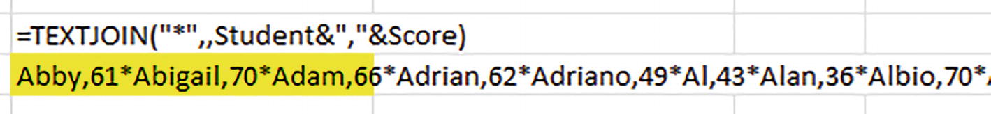
A screenshot of 2 spreadsheet rows. The formula for text join is entered in the top row. The highlighted text and number in the bottom row reads Abby, 61 asterisk Abigail, 70 asterisk Adam, 66.
Big class: 100 students and their scores, all joined in D4
(Now you can run a Copy > Paste Values atop D4.)
Note what the data currently look like. Each student name is followed by the test score on the other side of the comma. But each name/score is in turn separated from the next name/score by that asterisk – the delimiter we selected for TEXTJOIN. And now what?
=TEXTSPLIT(D4,",","*")

A cropped screenshot of a spreadsheet. Student names and their respective scores are split into 2 columns below the formula for text split.
The dataset, returned in full: names and test scores unlocked from D4 and reassigned to separate cells
Again, TEXTSPLIT splits the data in two directions: it seizes upon the comma column delimiter – grabbed from TEXTJOIN’s concatenation comma – to segregate the student names from their scores, and also applies TEXTJOIN’s own, official delimiter, the asterisk, to swing each record down to the next row by citing the asterisk in its “row delimiter” argument.
The larger point: TEXTSPLIT can skillfully break comma-separated values into functional data, but you can point that process in the other direction – retroactively define standard, separated data as a cohort of comma-separated values saved to one cell, and then recreate the dataset on an as needed-basis via TEXTSPLIT. That is, have TEXTJOIN round up hundreds or perhaps even thousands of records into one cell (remember an Excel cell can hold 32,767 characters) and retrieve them with TEXTSPLIT when you want to.
TEXTSPLIT Can’t Do Everything – but with Good Reason
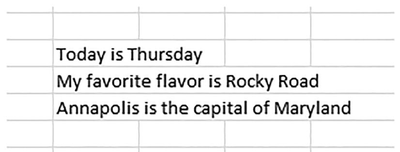
A partial screenshot of spreadsheet cells with 3 sentences written in 3 rows. The sentences from the top are, today is Thursday, my favorite flavor is rocky road, and Annapolis is the capital of Maryland.
Three cells to be split
=TEXTSPLIT(C7:C9, “ “)
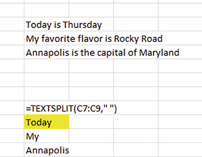
A cropped screenshot of a spreadsheet. The top has 3 sentences and bottom has a text-split formula and the words today, my, and Annapolis are entered in cells one below the other with today highlighted.
You can’t get there from here: TEXTSPLIT can’t split all the text from the three cells referenced by one formula.

A cropped screenshot of a spreadsheet. The cells on the extreme left column have sentences entered in them. The words in the sentences are split into the cells of the center columns. The formulas are entered in the extreme right column cells.
Splitting text, one line and one formula at a time

A screenshot of a spreadsheet column. The headers in the first cell are name, I d, and score. The scores for the names Bill, Jane, and Ed are entered. The I d for Bill in the second cell is missing.
No teacher’s pets: every student receives a TEXTSPLIT formula
Split the text via three TEXTSPLIT formulas, one each per row.
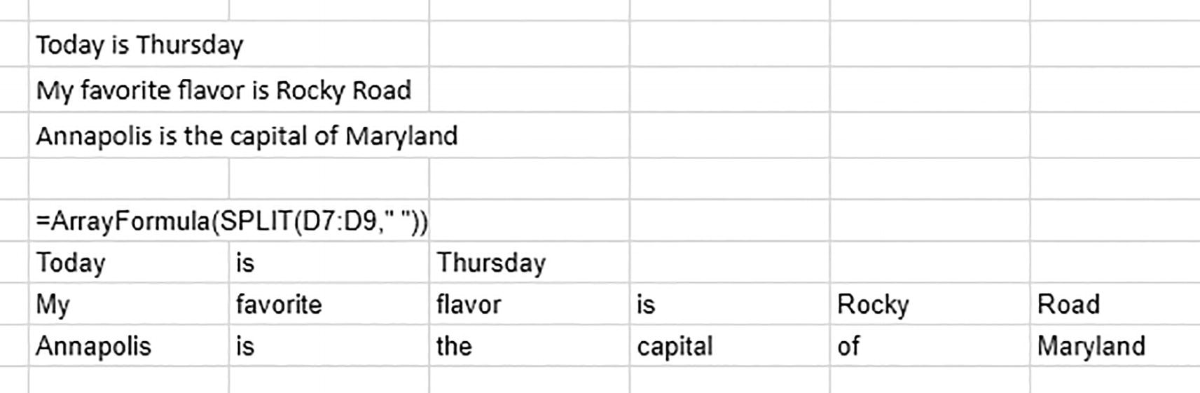
A screenshot of a spreadsheet. The formula entered in the center reads array formula left parenthesis split left parenthesis D 7 colon D 9, 2 double quotations right parenthesis right parenthesis. The words in the sentences above the formulae are split into cells below it.
Message from the competition: Google Sheets’ SPLIT function can split text in multiple cells with one formula
Why, then, can’t TEXSPLIT do the same?
=TEXTSPLIT(C7:C9, " ")
We see now that if the text in C7 were subjected to a row delimiter and hence spilled its words down the C column, its output would bump against and be obstructed by the text in C8, the next row down, and TEXTSPLIT can’t resolve that logjam. On the other hand, Google Sheet’s SPLIT function won’t be bothered by that complication – because it has no row delimiter to begin with.
There Is a Plan B
=TEXTSPLIT(TEXTJOIN("*",,C7:C9)," ","*",,,"")
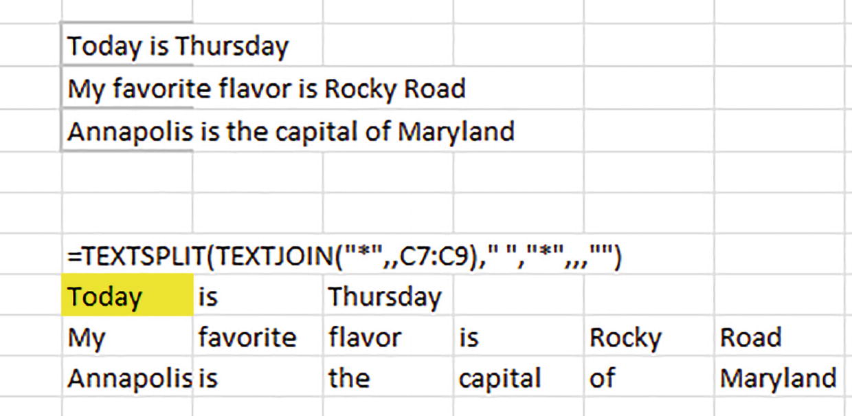
A screenshot of a spreadsheet. The top has 3 sentences. The formula for text split text join is entered below them. The words of the given sentences are split into individual cells below the formula. The cell with today in it is highlighted.
Breaking up isn’t that hard to do: the three text strings are knit together in one cell by TEXTJOIN, and then split into words with TEXTSPLIT
The linchpin to the formula is TEXTJOIN’s ability to stitch the three strings into a single cell, thus forging in effect one large text string. And that’s precisely the kind of object TEXTSPLIT is designed to handle – one text string in one cell. Thus, if we isolate the TEXTJOIN portion of the formula, we’ll see
Today is Thursday*My favorite flavor is Rocky Road*Annapolis is the capital of Maryland
And as with the earlier one-celled dataset example, TEXTJOIN registers the asterisk as its delimiter, which TEXTSPLIT in turn borrows for its own row delimiter, thus splitting the string back to its original three rows of text. TEXTSPLIT’s column delimiter – here the space – then divides each string into discrete words.
The formula’s final pair of quotes, the ones shunted to the far-right end of the formula, expresses the “pad with” argument. They’re needed here because the first text string – Today is Thursday – comprises just three words extending across three columns, while the other two strings and their six words naturally span six. And as explained earlier in the chapter, since “Today is Thursday” must also be afforded six columns – because every row in the spill range must exhibit the same number of columns – its three empty cells default to an #N/A message that can be overwritten with a “pad with” caption.
TEXTBEFORE and TEXTAFTER: Usefully Limiting the Delimiters
Cousins to the broader, more generic TEXTSPLIT, the new TEXTBEFORE and TEXTAFTER dynamic array functions offer a slightly narrower approach to the work of isolating specific text from cells, but presumably with a famed – or notorious – task specifically in mind, one to which we’ve already alluded.
That task: Taking full names crowded into a single cell and splitting them into first, middle, and last names – and TEXTBEFORE and TEXTAFTER stand ready to offer their able assistance. TEXTBEFORE returns text that appears before a specified instance of a delimiter, while TEXTAFTER travels in the opposite direction – it carries off text that follows a specified delimiter instance.
How They’re Written – and How They Work
=TEXTBEFORE(text,delimiter(s),instance number,match mode,match end,if not found)
{" ","*"}
And again, you can refer the delimiters to a table instead and supply the table name as a global delimiter name(s) in the formula.
The third argument, instance number, is central to the process. The number refers to the sequence position of a particular delimiter among all the delimiters in the cell. Simple example: the space delimiter preceding Sartre in the name John Paul Sartre is the second space in the cell proceeding from left to right, and as such would be designated 2 in TEXTBEFORE.
However, you can also note the instance number with a negative value, an option that initiates the delimiter count from the right end of the text and proceeds left, thus requiring a bit of a think-through. Working this way, that second space before Sartre would be coded -1 – meaning in this case that the space is the first delimiter in the cell pointing right to left. -2 in the same formula, then, would denote the second delimiter per the right-to-left orientation – and here, that would point to the space separating Jean and Paul. It sounds a bit obtuse, but as we’ll see, that reverse numbering scheme can serve you well.
And if you omit instance number altogether, TEXTBEFORE will work with the delimiter’s first instance by default.
TodayXisXThursday
=TEXTBEFORE(L14,"x")
(The other omitted arguments are optional.)
=TEXTBEFORE(L14,"x",,1)
Now apart from sounding like the conclusion of a sporting event, the fifth argument, “match end,” is trickier but can be put to productive use once you appreciate exactly what it does – something that took me a while. Inactive by default and denoted by the value 1 when it’s used, Microsoft says that “match end” “Treats the end of text as a delimiter,” a description that for me, at least, didn’t little to advance my understanding.
Today is Thursday[space]
And now that Excel has outfitted the string with the delimiter, TEXTBEFORE and TEXTAFTER can find it, and act upon it.
=TEXTBEFORE(A3," ")
=TEXTBEFORE(A4," ",,,1)
will station its virtual delimiter after the second “a” in Madonna. In effect, now, the formula will read Madonna as Madonna[space], and return all the text preceding that insurgent space – that is, Madonna.

A screenshot of spreadsheet cells. A sentence that reads today is Thursday is typed in the top left cell. Missing is entered in the bottom left cell. The formula for text before is entered in its right cell.
Attendance report: X is marked absent
TEXTAFTER: The Flip Side of TEXTBEFORE
TEXTAFTER, in effect a mirror image of TEXTBEFORE, sports the same syntax – with the essential distinction that the delimiter argument here seeks text that follows the appearance of the delimiter. Thus, for the space-delimited name John Doe, TEXTBEFORE will extract John – the name preceding the space, while TEXTAFTER will scrape the Doe, the text positioned after the space.
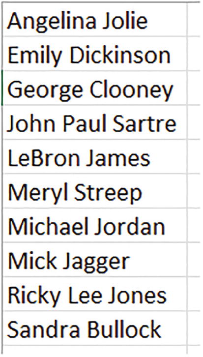
A screenshot of a spreadsheet column. The names entered in the column are Angelina Jolie, Emily Dickinson, George Clooney, John Paul Sartre, Le Bron James, Meryl Streep, Michael Jordan, Mick Jagger, Ricky Lee Jones, and Sandra Bullock.
The A-list
Our assignment here, a common one: to separate first from last names, while at the same time deciding where to position those thorny middle names that have been known to bedevil rosters and invitation lists.
Now in fact formula-based strategies for lifting first names from multi-name entries have long been in circulation, tying themselves to the LEFT and FIND functions. But TEXTS BEFORE and TEXTAFTER have some more lucid and elegant tricks up their sleeve, as we’ll see.
=TEXT BEFORE(A1:A10," ")
But wait. Didn’t we just learn just a few pages ago that a TEXTSPLIT formula was incapable of splitting text from multiple cells’ worth of data? We sure did. But TEXTS BEFORE and TEXTAFTER don’t suffer from that limitation. The absence of a row delimiter in TEXT BEFORE and TEXTAFTER means that they’ll never spill down and encroach upon the text in the cell beneath it – unlike TEXSPLIT.
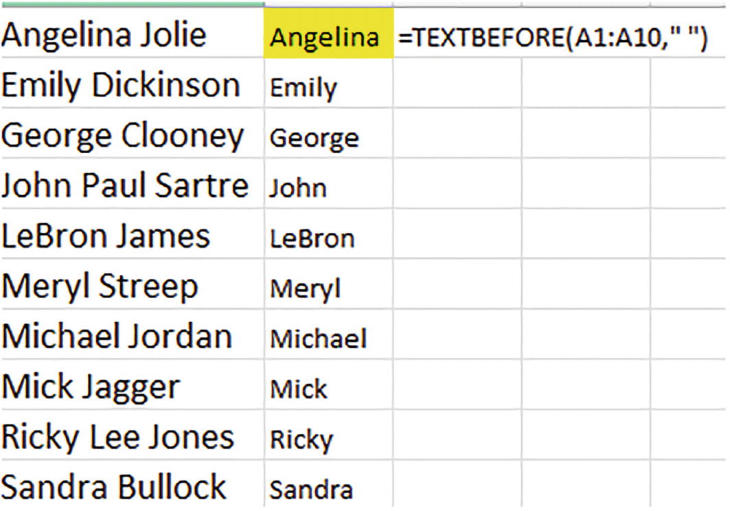
A cropped screenshot of a spreadsheet. The left column has a list of 10 names. The center column lists only the first names. The cell with Angelina in it is highlighted. The text before formula is entered in the right column.
Celebrities, on a first-name basis
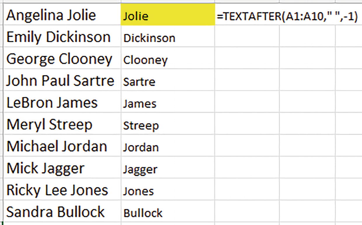
=TEXTAFTER(A1:A10," ")

A cropped screenshot of a spreadsheet. The first column has a list of 10 names. The second column lists only the first names. The third column lists only the last names. The text after formula is entered in the fourth column.
Big Sur: surnames via TEXT AFTER
Here by default TEXT AFTER sights the first space in each respective name, and fills each cell with all the text to the space’s right.
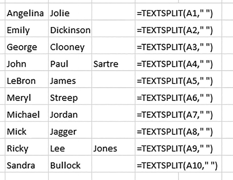
A cropped screenshot of a spreadsheet. The first column lists the first names. The second column lists the last names. The third column has 2 extra last names for John and Ricky. The fourth column has the formulae for text split for the corresponding cells.
Having second thoughts about second names? Splitting names with TEXTSPLIT
Probably not what you had in mind – because while TEXTSPLIT manages to split each and every name, the two middle names share column B with most of the surnames.
Front and Center: Extracting Middle Names

A cropped screenshot of a spreadsheet. The first column lists full names. The second column lists the first names. The third column lists the middle names. The fourth column lists the last names.
Caught in the middle: middle names captured as well
That ambition is a little grander, because the TEXT BEFORE/AFTER functions spirit away all of the text on either side of a delimiter. But here we want to glean text wedged between two delimiters, surrounded by unwanted text on either side.
=TEXTAFTER(TEXT BEFORE(A1:A10," ",-1)," ",,,1)

A screenshot of 2 spreadsheet columns. The left column lists some first names. The top-left cell with Angelina in it is highlighted. The formula for text before is entered in the top right cell.
The right stuff: text returned from left of the rightmost space in each name
Of course these are mid-way results, forming a temporary, virtual dataset that supplies names – each of which now features, or will feature, but one space – upon which the TEXT AFTER half of the formula is about to act.
And when we wrap TEXT AFTER around TEXTBEFORE, the formula now examines the names pictured above and simply yanks the text following the one and only space remaining within each name. In the case of John Paul, then, the name Paul is returned; in the case of the cells bearing only one name, again the “match end” delimiter latches its faux space to the end of the name – and TEXTAFTER discovers nothing after it, leaving the cell blank.
Sorting Last Names: Sort of Tricky
=SORTBY(A1:A10,TEXTAFTER(A1:A10," ",-1))
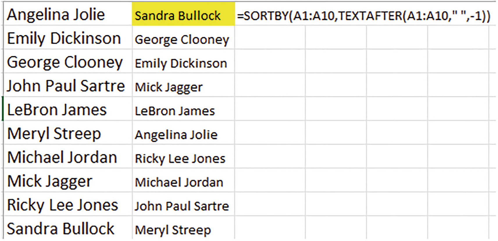
A cropped screenshot of a spreadsheet. Two columns list some names. The names are arranged in alphabetical order with respect to the first names in column 1 and last names in column 2. The sort by formula is entered in column 3.
Internal alphabetical order: sorting by last names
A cropped screenshot of a spreadsheet. The left column lists some names. The center column lists only the last names. The cell with Jolie in it is highlighted. The formula for text after is entered in the right cell.
Behind the scenes: this part of the formula sorts last names only
It then proceeds in effect to sort the two columns – that is, the actual data in A and the virtual column of last names returned inside the formula – by the latter, which brings the first-column names, the ones we actually view in the worksheet along for the ride.
Some Concluding Words
Number crunching may be Excel’s stock in trade, but as we’ve seen there’s plenty of work it can do with words, too; and the new text functions strive to make that work simpler and more productive.
The next pair of new dynamic array functions, TOCOL and TOROW, flattens multi-column or multi-row ranges into a single column or row. And you’ll see why you’ll want to add these new terms to your spreadsheet vocabulary.