
To reiterate an introductory point we made a short while ago: Excel’s new, second-generation dynamic array functions don’t open many new windows on number crunching; rather, they’re primarily about revamping and streamlining the way in which data can be organized. And that’s a point that surely calls for some explanation, beginning with a description of the TOROW and TOCOL functions.
How They’re Written – and What They’re About
TOCOL and TOROW were crafted to allow users simpler means for analyzing data that’s currently committed to a rectangular form. So what does that mean?

A matrix with 4 columns and 12 rows filled with integers from 1 to 10. The row entries are as follows. Row 1. 1, 3, 9, and 7. Row 2. 2, 5, 6, and 3. Row 3. 3, 4, 8, and 7. Row 4. 9, 2, 3, and 4. So on.
The matrix: the sequel
We want to count the frequency with which each value appears in the range, but the dispersion of those values across five columns makes the exercise something of a pause giver – because before we can count each value with the standard COUNTIF function we need to list each value uniquely as criteria, so that COUNTIF knows what it’s counting; and assembling a unique list of values across columns is no straightforward thing.
Enter TOCOL, which is happy to throw itself at multi-column data and distill them all into a single column, after which all kinds of data-analytic tasks become much easier. After all, once you’ve somehow squeezed all the above values into one column – even temporarily – the UNIQUE function can fearlessly spring into action.
=TOCOL(range/array,ignore,scan by column)
The first argument, range, or what Excel again terms “array,” simply requests the coordinates of the data with which TOCOL is to work – that is, which data will be reshaped into a single column.
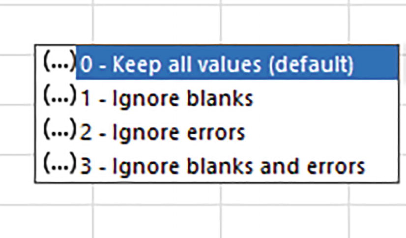
A set of 4 options. 0, keep all values default. 1, ignore blanks. 2, ignore errors. 3, ignore blanks and errors. 0, keep all values default is selected.
TOCOL ignore options; don’t ignore them
The first as conveyed by the 0, Keep all values, serves as the default option and can be omitted; it simply preserves all existing values in the range/array and will return them all to the single column TOCOL will construct. Ignore blanks does just that, that is, it forsakes any empty cells in the source range/array and bars them from the TOCOL result, and ignore errors does the same for error-message-bearing cells. The fourth option, ignore blanks and errors, combines the operations of options 2 and 3.
=TOCOL(G6:J27)
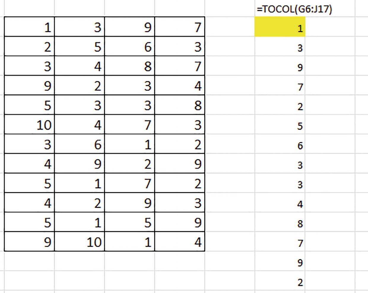
A matrix of 4 columns and 12 rows is highlighted in an excel sheet. A list of numbers is under an excel formula. The formula reads, equals T O C O L left parenthesis G 6 colon J 17 right parenthesis.
All four one – the matrix narrowed to a single column
=TOCOL(G6:J17,,1)
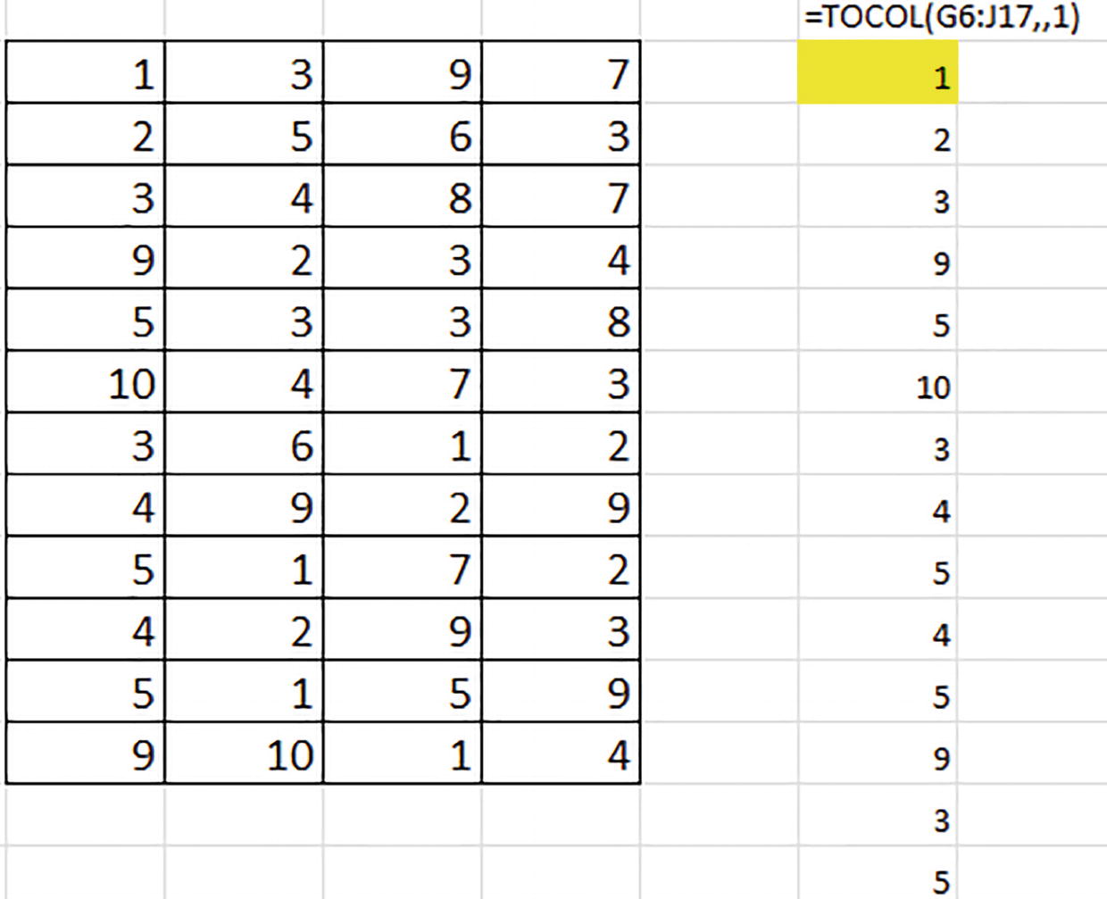
A table of 4 columns and 12 rows and a list of numbers with an Excel formula. The formula reads equals T O C O L left parenthesis G 6 colon J 17 comma comma 1 right parenthesis. 1 in the first cell under the formula is highlighted.
Heading in a different direction: the results dive down the columns for their results
Here, the first four TOCOL results capture the 1, 2, 3, and 9 from the matrix’ first column, because the values are searched downwards.

A table of 4 columns and 12 rows and a list of numbers with an Excel formula. The formula reads equals SORT left parenthesis unique left parenthesis T O C O L left parenthesis G 6 colon J 17 comma comma 1 close all the parentheses.
Each matrix value – once each, in numerical order
=COUNTIF(G6:J17,L6#)
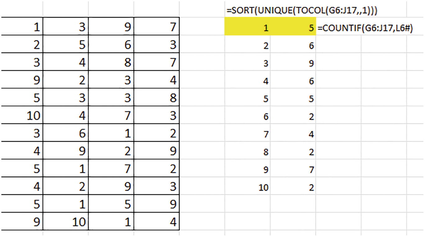
A table of 4 columns and 12 rows and two lists of numbers with two Excel formulas. One of the formulas read equals SORT left parenthesis unique left parenthesis T O C O L left parenthesis G 6 colon J 17,,1 close all parentheses.
Matrix values, ac-counted for
Mission accomplished. We’ve brought the TOCOL function to bear on multi-column data, thus enabling us to easily collect unique instances of each value.
Now what if we wanted to sort the matrix values – within the multi-columned matrix? That’s also something we can do, but that assignment awaits the next chapter, in which we debut the WRAPCOLS and WRAPROWS functions and partner them with TOCOL
Drawing a Bead on the Blanks

A table of 5 columns and 11 rows. The column headers are Monday, Tuesday, Wednesday, Thursday, and Friday. Columns are recorded with names.
Classifying daily attendance data
=SORT(UNIQUE(TOCOL(A2:E11)))

A list of names with an Excel formula. The formula reads equals SORT left parenthesis unique left parenthesis T O C O L left parenthesis A 2 colon E 11 close all parentheses. Bennie's name was highlighted.
Ten students, eleven outcomes

A list of names with an Excel formula. The formula reads equals SORT left parenthesis unique left parenthesis T O C O L left parenthesis A 2 colon E 11, 1 close all right parentheses. Bennie was highlighted.
All present and accounted for – except the blanks
evicts any blanks from the spill range, a happy consequence of the 1 we’ve added to the formula (the “ignore blanks” argument), and that looks much better.
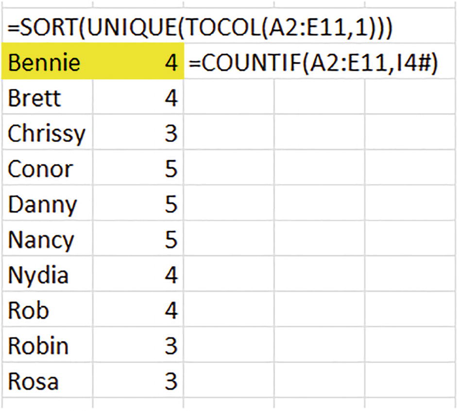
A list of names and a list of numbers with formulas equal SORT left parenthesis unique left parenthesis T O C O L left parenthesis A 2 colon E 11, 14 hash right parenthesis. Bennie and number 4 are highlighted.
Gold stars for Conor, Danny, and Nancy

A table of 5 columns and 11 rows. The column headers are Monday, Tuesday, Wednesday, Thursday, and Friday. A list of names and numbers with formulas is mentioned with Bennie and 4 highlighted.
Zelda is new, reported, and sorted
TOROW Is Slightly Different
And as you’ve probably inferred, TOROW realigns multi-column data into a single row’s worth of output, relying on the same arguments as TOCOL but nevertheless sometimes requiring a few more user decisions.

A row of names with an Excel formula. Names are Bennie, Brett, Chrissy, Conor, Danny, Nancy, Nydia, Rob, Robin, and Rosa. The formula reads equals SORT left parenthesis UNIQUE left parenthesis and so on.
Sideways student sort
What’s different here is that the UNIQUE function must be told to spill the unique names across columns, evidenced by the 1 in its final argument (the one preceding the three commas); and SORT too must be asked to order the data horizontally – stipulated by the last 1 in the entire formula.
By default, both TOCOL and TOROW scan the ranges which they work by column; that is, they scan the data horizontally, realigning them into a single column or row one column at a time.
Lining Up the Conclusions

A table of 2 columns and 3 rows. The row entries are as follows. Row 1. Ted, 56. Row 2. Jane, 67. Row 3. Mary, 87.
Don’t try this at home: jamming two fields into one column

A table of 1 column and 6 rows. The column entry is as follows. Ted, 56, Jane, 67, Mary, and 87.
Apples and oranges: Alphas and numerics don’t mix
Try that and you’ll be reaching for the undo command pronto.
Coming Attractions
The next chapter will introduce a pair of new functions that can be made to usefully partner with TOCOL and TOROW, WRAPCOLS and WRAPROWS, both of which take the analysis in the opposite direction – by spreading one column’s or row’s worth of data into multiple columns or rows.