7
Solution Procedure: Integral Transform Methods
7.1 INTRODUCTION
Integral transforms are considered to be operational methods or operational calculus methods that are developed for the efficient solution of differential and integral equations. In these methods, the operations of differentiation and integration are symbolized by algebraic operators. Oliver Heaviside (1850–1925) was the first person to develop and use the operational methods for the solution of the telegraph equation and the second‐order hyperbolic partial differential equations with constant coefficients in 1892 [1]. However, his operational methods were based mostly on intuition and lacked mathematical rigor. Although subsequently, the operational methods have developed into one of most useful mathematical methods, contemporary mathematicians hardly recognized Heaviside's work on operational methods, due to its lack of mathematical rigor.
Subsequently, many mathematicians have tried to interpret and justify Heaviside's work. For example, Bromwich and Wagner tried to justify Heaviside's work on the basis of contour integration [2,3]. Carson attempted to derive the operational method using an infinite integral of the Laplace type [4]. Van der Pol and other mathematicians tried to derive the operational method by employing complex variable theory [5]. All these attempts proved successful in establishing the mathematical validity of the operational method in the early part of the twentieth century. As such, the modern concept of the operational method has a rigorous mathematical foundation and is based on the functional transformation provided by Laplace and Fourier integrals.
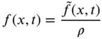
In general, if a function ![]() , defined in terms of the independent variable t, is governed by a differential equation with certain initial or boundary conditions, the integral transforms convert
, defined in terms of the independent variable t, is governed by a differential equation with certain initial or boundary conditions, the integral transforms convert ![]() into
into ![]() defined by
defined by
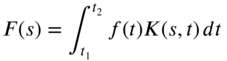
where s is a parameter, ![]() is called the kernel of the transformation, and
is called the kernel of the transformation, and ![]() and
and ![]() are the limits of integration. The transform is said to be finite if
are the limits of integration. The transform is said to be finite if ![]() and
and ![]() are finite. Equation (7.1) is called the integral transformation of
are finite. Equation (7.1) is called the integral transformation of ![]() . It converts a differential equation into an algebraic equation in terms of the new, transformed function
. It converts a differential equation into an algebraic equation in terms of the new, transformed function ![]() . The initial or boundary conditions will be accounted for automatically in the process of conversion to an algebraic equation. The resulting algebraic equation can be solved for
. The initial or boundary conditions will be accounted for automatically in the process of conversion to an algebraic equation. The resulting algebraic equation can be solved for ![]() without much difficulty. Once
without much difficulty. Once ![]() is known, the original function
is known, the original function ![]() can be found by using the inverse integral transformation.
can be found by using the inverse integral transformation.
If a function f, defined in terms of two independent variables, is governed by a partial differential equation, the integral transformation reduces the number of independent variables by one. Thus, instead of a partial differential equation, we need to solve only an ordinary differential equation, which is much simpler. A major task when using the integral transform method involves carrying out the inverse transformation. The transform and its inverse are called the transform pair. The most commonly used integral transforms are the Fourier and Laplace transforms. The application of both these transforms for the solution of vibration problems is considered in this chapter.
7.2 FOURIER TRANSFORMS
7.2.1 Fourier Series
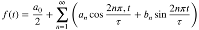
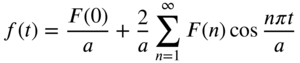
In Section 1.10 we saw that the Fourier series expansion of a function ![]() that is periodic with period
that is periodic with period ![]() and contains only a finite number of discontinuities is given by
and contains only a finite number of discontinuities is given by
where the coefficients ![]() and
and ![]() are given by
are given by

Using the identities

Eq. (7.2) can be expressed as

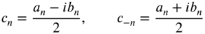
where ![]() . By defining the complex Fourier coefficients
. By defining the complex Fourier coefficients ![]() and
and ![]() as
as
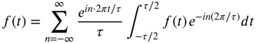
Eq. (7.5) can be expressed as

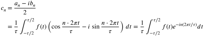
where the Fourier coefficients ![]() can be determined using Eqs. (7.3) as
can be determined using Eqs. (7.3) as
7.2.2 Fourier Transforms
When the period of the periodic function ![]() in Eq. (7.9) is extended to infinity, the expansion will be applicable to nonperiodic functions as well. For this, let
in Eq. (7.9) is extended to infinity, the expansion will be applicable to nonperiodic functions as well. For this, let ![]() and
and ![]() . As
. As ![]() and the subscript n need not be used since the discrete value of
and the subscript n need not be used since the discrete value of ![]() becomes continuous. By using the relations
becomes continuous. By using the relations ![]() and
and ![]() as
as ![]() , Eq. (7.9) becomes
, Eq. (7.9) becomes

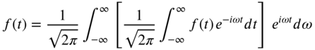
Equation (7.10), called the Fourier integral, is often expressed in the form of the following Fourier transform pair:


where ![]() is called the Fourier transform of
is called the Fourier transform of ![]() and
and ![]() is called the inverse Fourier transform of
is called the inverse Fourier transform of ![]() . In Eq. (7.12),
. In Eq. (7.12), ![]() can be considered as the harmonic contribution of the function
can be considered as the harmonic contribution of the function ![]() in the frequency range
in the frequency range ![]() to
to ![]() . This also denotes the limiting value of
. This also denotes the limiting value of ![]() as
as ![]() , as indicated by Eq. (7.8). Thus, Eq. (7.12) denotes an infinite sum of harmonic oscillations in which all frequencies from
, as indicated by Eq. (7.8). Thus, Eq. (7.12) denotes an infinite sum of harmonic oscillations in which all frequencies from ![]() to
to ![]() are represented.
are represented.
Notes
- By rewriting Eq. (7.10) as
(7.13)
the Fourier transform pair can be defined in a symmetric form as
(7.15)
It is also possible to define the Fourier transform pair as
(7.16)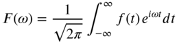 (7.17)
- The Fourier transform pair corresponding to an even function
 can be defined as follows:
(7.18)
can be defined as follows:
(7.18)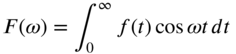 (7.19)
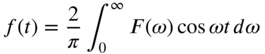
The Fourier sine transform pair corresponding to an odd function
 can be defined as(7.20)
 (7.21)
- The Fourier transform pair is applicable only to functions
 that satisfy Dirichlet's conditions in the range
  . A function
  is said to satisfy Dirichlet's conditions in the interval
  if (a)
  has only a finite number of maxima and minima in
  and
and  has only a finite number of finite discontinuities with no infinite discontinuity in
  . As an example, the function
  satisfies Dirichlet's conditions in the interval
  , whereas the function
  does not satisfy Dirichlet's conditions in any interval containing the point
  because
  has an infinite discontinuity at
  .
.

7.2.3 Fourier Transform of Derivatives of Functions
Let the Fourier transform of the jth derivative of the function ![]() be denoted as
be denoted as ![]() . Then, by using the definition of Eq. (7.11),
. Then, by using the definition of Eq. (7.11),
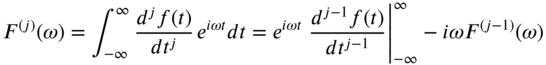
Assuming that the ![]() derivative of
derivative of ![]() is zero as
is zero as ![]() , Eq. (7.22) reduces to
, Eq. (7.22) reduces to
Again assuming that all derivatives of order ![]() are zero as
are zero as ![]() , Eq. (7.23) yields
, Eq. (7.23) yields
where ![]() is the complex Fourier transform of
is the complex Fourier transform of ![]() given by Eq. (7.11).
given by Eq. (7.11).
7.2.4 Finite Sine and Cosine Fourier Transforms
The Fourier series expansion of a function ![]() in the interval
in the interval ![]() is given by [using Eq. (1.32)]
is given by [using Eq. (1.32)]
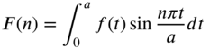
where

Using Eqs. (7.25) and (7.26), the finite cosine Fourier transform pair is defined as


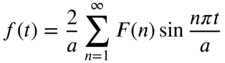
A similar procedure can be used to define the finite sine Fourier transforms. Starting with the Fourier sine series expansion of a function ![]() defined in the interval
defined in the interval ![]() (using Eq. [(7.32)]), we obtain
(using Eq. [(7.32)]), we obtain

where
the finite sine Fourier transform pair is defined as


When the independent variable t is defined in the range ![]() instead of
instead of ![]() , the finite cosine transform is defined as
, the finite cosine transform is defined as
where ![]() is yet unspecified. Defining a new variable y as
is yet unspecified. Defining a new variable y as ![]() so that
so that ![]() , Eq. (7.33) can be rewritten as
, Eq. (7.33) can be rewritten as

where
If ![]() or
or ![]() , then
, then
Returning to the original variable t, we define the finite cosine transform pair as

Similarly, the finite sine Fourier transform pair is defined as
7.3 FREE VIBRATION OF A FINITE STRING
Consider a string of length l under tension P and fixed at the two endpoints ![]() and
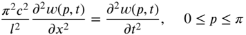
and ![]() . The equation of motion governing the transverse vibration of the string is given by
. The equation of motion governing the transverse vibration of the string is given by

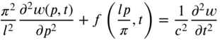
By redefining the spatial coordinate x in terms of p as
Eq. (7.41) can be rewritten as
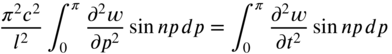
We now take finite sine transform of Eq. (7.43). According to Eq. (7.31), we multiply Eq. (7.43) by sin np and integrate with respect to p from 0 to ![]() :
:
where

Since the string is fixed at ![]() and
and ![]() , the first term on the right‐hand side of Eq. (7.45) vanishes, so that
, the first term on the right‐hand side of Eq. (7.45) vanishes, so that
Thus, Eq. (7.44) becomes

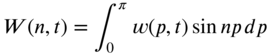
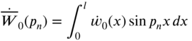
Defining the finite Fourier sine transform of ![]() as (see Eq. [7.31])
as (see Eq. [7.31])

Eq. (7.47) can be expressed as an ordinary differential equation as

The solution of Eq. (7.49) is given by
or
where the constants ![]() and
and ![]() or
or ![]() and
and ![]() can be determined from the known initial conditions of the string.
can be determined from the known initial conditions of the string.
Let the initial conditions of the string be given by
In terms of the finite Fourier sine transform ![]() defined by Eq. (7.48), Eqs. (7.51) and (7.52) can be expressed as
defined by Eq. (7.48), Eqs. (7.51) and (7.52) can be expressed as
where

or


or
Equations (7.53), (7.54), and (7.50) lead to
Thus, the solution, Eq. (7.50), becomes
The inverse finite Fourier sine transform of ![]() is given by (see Eq. [7.32])
is given by (see Eq. [7.32])

Substituting Eq. (7.61) into (7.62), we obtain

Using Eqs. (7.56) and (7.58), Eq. (7.63) can be expressed in terms of x and t as
7.4 FORCED VIBRATION OF A FINITE STRING
Consider a string of length l under tension P, fixed at the two endpoints ![]() and
and ![]() , and subjected to a distributed transverse force
, and subjected to a distributed transverse force ![]() . The equation of motion of the string is given by (see Eq. [8.7])
. The equation of motion of the string is given by (see Eq. [8.7])

or

where
As in Section (7.3), we change the spatial variable x to p as
so that Eq. (7.66) can be written as
By proceeding as in the case of free vibration (Section (7.3)), Eq. (7.69) can be expressed as an ordinary differential equation:

where
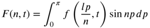
Assuming the initial conditions of the string to be zero, the steady‐state solution of Eq. (7.70) can be expressed as
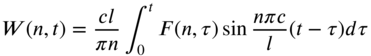
The inverse finite Fourier sine transform of ![]() is given by (see Eq. [7.32])
is given by (see Eq. [7.32])

or

7.5 FREE VIBRATION OF A BEAM
Consider a uniform beam of length l simply supported at ![]() and
and ![]() . The equation of motion governing the transverse vibration of the beam is given by (see Eq. [3.19])
. The equation of motion governing the transverse vibration of the beam is given by (see Eq. [3.19])

where

The boundary conditions can be expressed as

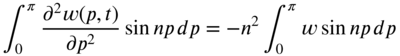
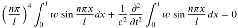
We take the finite Fourier sine transform of Eq. (7.76). For this, we multiply Eq. (7.76) by ![]() and integrate with respect to x from 0 to l:
and integrate with respect to x from 0 to l:
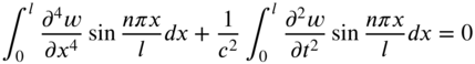
Here
In view of the boundary conditions of Eq. (7.79), Eq. (7.81) reduces to

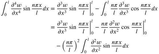
Again, using integration by parts, the integral on the right‐hand side of Eq. (7.82) can be expressed as
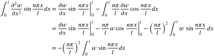
in view of the boundary conditions of Eq. (7.78). Thus, Eq. (7.80) can be expressed as
Defining the finite Fourier sine transform of ![]() as (see Eq. [7.39])
as (see Eq. [7.39])

Eq (7.84) reduces to the ordinary differential equation
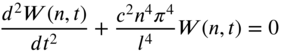
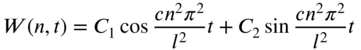
The solution of Eq. (7.86) can be expressed as
or
Assuming the initial conditions of the beam as
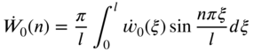
the finite Fourier sine transforms of Eqs. (7.89) and (7.90) yield
where


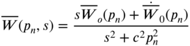
Using the initial conditions of Eqs. (7.93) and (7.94), Eq. (7.88) can be expressed as

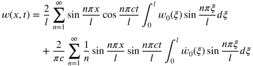
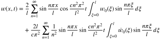
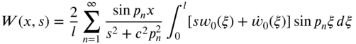
Finally, the transverse displacement of the beam, ![]() , can be determined by using the finite inverse Fourier sine transform of Eq. (7.95) as
, can be determined by using the finite inverse Fourier sine transform of Eq. (7.95) as

which can be rewritten, using Eqs. (7.93) and (7.94), as
7.6 LAPLACE TRANSFORMS
The Laplace transform technique is an operational method that can be used conveniently to solve linear ordinary differential equations with constant coefficients. The method can also be used for the solution of linear partial differential equations that govern the response of continuous systems. Its advantage lies in the fact that differentiation of the time function corresponds to multiplication of the transform by a complex variable s. This reduces a differential equation in time t to an algebraic equation in s. Thus, the solution of the differential equation can be obtained by using either a Laplace transform table or the partial fraction expansion method. An added advantage of the Laplace transform method is that during the solution process, the initial conditions of the differential equation are taken care of automatically, so that both the homogeneous (complementary) solution and the particular solution can be obtained simultaneously.
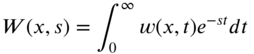
The Laplace transformation of a time‐dependent function, ![]() , denoted as
, denoted as ![]() , is defined as
, is defined as
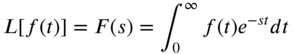
where L is an operational symbol denoting that the quantity upon which it operates is to be transformed by the Laplace integral

The inverse or reverse process of finding the function ![]() from the Laplace transform
from the Laplace transform ![]() , known as the inverse Laplace transform, is donated as
, known as the inverse Laplace transform, is donated as

Certain conditions are to be satisfied for the existence of the Laplace transform of the function ![]() . One condition is that the absolute value of
. One condition is that the absolute value of ![]() must be bounded as
must be bounded as
for some constants C and ![]() . This means that if the values of the constants C and
. This means that if the values of the constants C and ![]() can be found such that
can be found such that
then

Another condition is that the function ![]() must be piecewise continuous. This means that in a given interval, the function
must be piecewise continuous. This means that in a given interval, the function ![]() has a finite number of finite discontinuities and no infinite discontinuity.
has a finite number of finite discontinuities and no infinite discontinuity.
7.6.1 Properties of Laplace Transforms
Some of the important properties of Laplace transforms are indicated below.
- Linearity property. If
 and
and  are any constant and
  and
and  are functions of t with Laplace transforms
  and
and  , respectively, then
The validity of Eq. (7.104) can be seen from the definition of the Laplace transform. Because of this property, the operator L can be seen to be a linear operator.
- First translation or shifting property. If
 for
for  , then
where
 and a may be a real or complex number. To see the validity of Eq. (7.105), we use the definition of the Laplace transform(7.106)
Equation (7.105) shows that the effect of multiplying
 by
by  in the real domain is to shift the transform of
  by an amount a in the s‐domain.
 - Second translation or shifting property. If
then
 (7.107)
- Laplace transformation of derivatives. If
 , then
To see the validity of Eq. (7.108), we use the definition of Laplace transform as
Integrating the right‐hand side of Eq. (7.109) by parts, we obtain
(7.110)
The property of Eq. (7.108) can be extended to the nth derivative of
 to obtain(7.111)
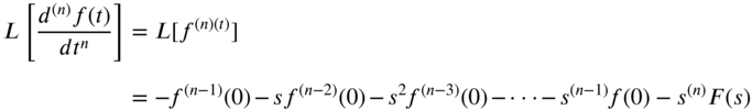
where
(7.112)
- Convolution theorem. Let the Laplace transforms of the functions
 and
and  be given by
  and
and  , respectively. Then
where
 is called the convolution or the faltung of F and G. Equation (7.113) can be expressed equivalently as(7.114)
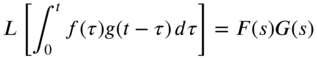
or conversely,
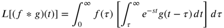
To prove the validity of Eqs. (7.113)–(7.115), consider the definition of the Laplace transform and the convolution operation as
From the region of integration shown in Fig. 7.1, the integral in Eq. (7.116) can be rewritten, by interchanging the order of integration, as
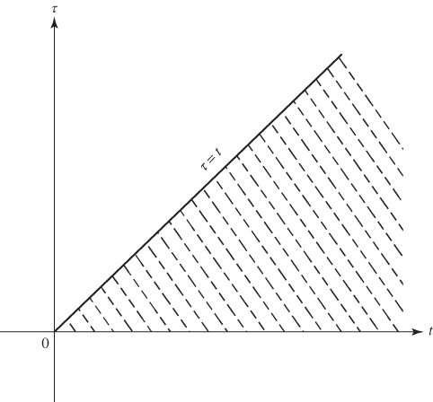
Figure 7.1 Region of integration in Eq. (7.116).
By using the second property, the inner integral can be written as
 , so that Eq. (7.117) can be expressed as(7.118)
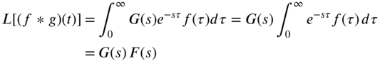
The converse result can be stated as
(7.119)


7.6.2 Partial Fraction Method
In the Laplace transform method, sometimes we need to find the inverse transformation of the function
where ![]() and
and ![]() are polynomials in s with the degree of
are polynomials in s with the degree of ![]() less than that of
less than that of ![]() . Let the polynomial
. Let the polynomial ![]() be of order n with roots
be of order n with roots ![]() , so that
, so that
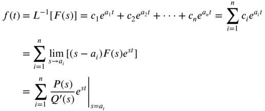
First, let us consider the case in which all the n roots ![]() are distinct, so that Eq. (7.120) can be expressed as
are distinct, so that Eq. (7.120) can be expressed as

where ![]() are coefficients. The points
are coefficients. The points ![]() are called simple poles of
are called simple poles of ![]() .
.
The poles denote points at which the function ![]() becomes infinite. The coefficients
becomes infinite. The coefficients ![]() in Eq. (7.122) can be found as
in Eq. (7.122) can be found as
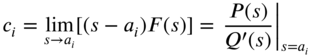
where ![]() is the derivative of
is the derivative of ![]() with respect to s. Using the result
with respect to s. Using the result
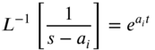
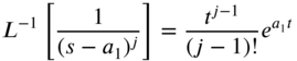
the inverse transform of Eq. (7.122) can be found as
Next, let us consider the case in which ![]() has a multiple root of order k, so that
has a multiple root of order k, so that
In this case, Eq. (7.120) can be expressed as

Note that the coefficients ![]() can be determined as
can be determined as
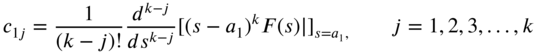
while the coefficients ![]() ,
, ![]() , can be found as in Eq. (7.125). Since
, can be found as in Eq. (7.125). Since
the inverse of Eq. (7.127) can be expressed as

7.6.3 Inverse Transformation
The inverse Laplace transformation, denoted as ![]() , is also defined by the complex integration formula
, is also defined by the complex integration formula

where ![]() is a suitable real constant, in Eq. (7.131), the path of the integration is a line parallel to the imaginary axis that crosses the real axis at Re
is a suitable real constant, in Eq. (7.131), the path of the integration is a line parallel to the imaginary axis that crosses the real axis at Re ![]() and extends from
and extends from ![]() to
to ![]() . We assume that
. We assume that ![]() is an analytic function of the complex variable s in the right half‐plane Re
is an analytic function of the complex variable s in the right half‐plane Re ![]() and all the poles lie to the left of the line
and all the poles lie to the left of the line ![]() . This condition is usually satisfied for all physical problems possessing stability since the poles to the right of the imaginary axis denote instability. The details of evaluation of Eq. (7.131) depend on the nature of the singularities of
. This condition is usually satisfied for all physical problems possessing stability since the poles to the right of the imaginary axis denote instability. The details of evaluation of Eq. (7.131) depend on the nature of the singularities of ![]() .
.
The path of the integration is the straight line ![]() , as shown in Fig. 7.2, in the complex s plane, with equation
, as shown in Fig. 7.2, in the complex s plane, with equation ![]() and Re
and Re ![]() is chosen so that all the singularities of the integrand of Eq. (7.131) lie to the left of the line
is chosen so that all the singularities of the integrand of Eq. (7.131) lie to the left of the line ![]() . The Cauchy‐residue theorem is used to evaluate the contour integral as
. The Cauchy‐residue theorem is used to evaluate the contour integral as
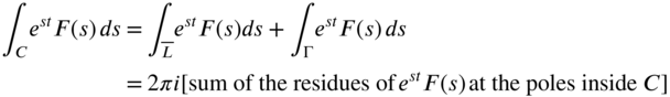
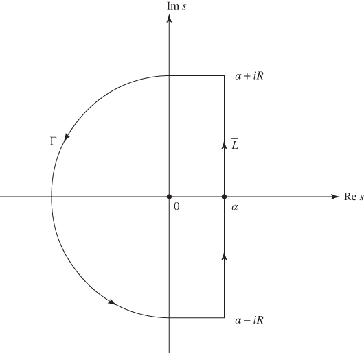
Figure 7.2 Contour of integration.
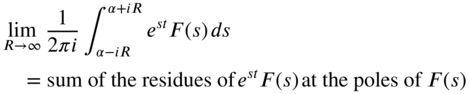
where ![]() and the integral over
and the integral over ![]() tends to zero in most cases. Thus, Eq. (7.131) reduces to the form
tends to zero in most cases. Thus, Eq. (7.131) reduces to the form
Example 7.5 illustrates the procedure of contour integration.
7.7 FREE VIBRATION OF A STRING OF FINITE LENGTH
In this case, the equation of motion is
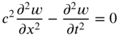
If the string is fixed at ![]() and
and ![]() , the boundary conditions are
, the boundary conditions are
Let the initial conditions of the string be given by
Applying Laplace transforms to Eq. (7.134), we obtain
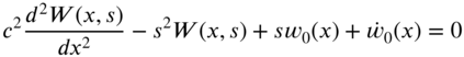
where
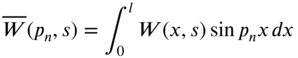
Taking finite Fourier sine transform of Eq. (7.139), we obtain
where

with
Eq. (7.141) gives
Performing the inverse finite Fourier sine transform of Eq. (7.146) yields
Finally, by taking the inverse Laplace transform of ![]() in Eq. (7.147), we obtain
in Eq. (7.147), we obtain

7.8 FREE VIBRATION OF A BEAM OF FINITE LENGTH
The equation of motion for the transverse vibration of a beam is given by

where

For free vibration, ![]() is assumed to be harmonic with frequency
is assumed to be harmonic with frequency ![]() :
:
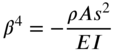
so that Eq. (7.149) reduces to an ordinary differential equation:
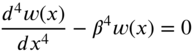
where

By taking Laplace transforms of Eq. (7.152), we obtain
or
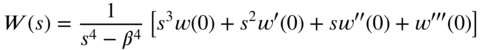
where ![]() , and
, and ![]() denote the deflection and its first, second, and third derivative, respectively, at
denote the deflection and its first, second, and third derivative, respectively, at ![]() . By noting that
. By noting that
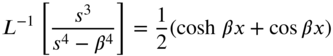


the inverse Laplace transform of Eq. (7.155) gives

7.9 FORCED VIBRATION OF A BEAM OF FINITE LENGTH
The governing equation is given by

where ![]() denotes the time‐varying distributed force. Let the initial deflection and velocity be given by
denotes the time‐varying distributed force. Let the initial deflection and velocity be given by ![]() and
and ![]() , respectively. The Laplace transform of Eq. (7.161), with respect to t with s as the subsidiary variable, yields
, respectively. The Laplace transform of Eq. (7.161), with respect to t with s as the subsidiary variable, yields

or
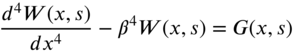
where
Again, by taking the Laplace transform of Eq. (7.163) with respect to x with p as the subsidiary variable, we obtain

or

where ![]() ,
, ![]() ,
, ![]() , and
, and ![]() denote the Laplace transforms with respect to t of
denote the Laplace transforms with respect to t of ![]() and
and ![]() respectively, at
respectively, at ![]() . Next, we perform the inverse Laplace transform of Eq. (7.166) with respect to x. For this, we use Eqs. (7.156) –(7.159) and express the inverse transform of Eq. (7.166) as
. Next, we perform the inverse Laplace transform of Eq. (7.166) with respect to x. For this, we use Eqs. (7.156) –(7.159) and express the inverse transform of Eq. (7.166) as
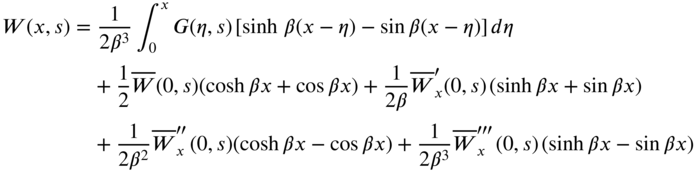
Finally, we perform the inverse Laplace transform of Eq. (7.167) with respect to t to find the desired solution, ![]() . The procedure is illustrated in Example 7.7.
. The procedure is illustrated in Example 7.7.
7.10 RECENT CONTRIBUTIONS
Fast Fourier transforms: The fast Fourier transform algorithm and the associated programming considerations in the calculation of sine, cosine, and Laplace transforms were presented by Cooley et al. [13]. The problem of establishing the correspondence between discrete and continuous functions is described.
Beams: Cobble and Fang [14] considered the finite transform solution of the damped cantilever beam equation with distributed load, elastic support, and the wall edge elastically restrained against rotation. The solution is based on the properties of a Hermitian operator and its orthogonal basis vectors.
Membranes: The general solution of the vibrating annular membrane with arbitrary loading, initial conditions, and time‐dependent boundary conditions was given by Sharp [15].
Hankel transform: The solution of the scalar wave equation of an annular membrane, in which the motion is symmetrical about the origin, for arbitrary initial and boundary conditions was given in Ref. [16]. The solution is obtained by using a finite Hankel transform. An example is given to illustrate the procedure and the solution is compared to the one given by the method of separation of variables.
Plates: A method of determining a finite integral transform that will remove the presence of one of the independent variables in a fourth‐order partial differential equation is applied to the equation of motion of classical plate theory for complete and annular circular plates subjected to various boundary conditions by Anderson [17]. The method is expected to be particularly useful for the solution of plate vibration problems with time‐dependent boundary conditions. Forced torsional vibration of thin, elastic, spherical, and hemispherical shells subjected to either a free or a restrained edge was considered by Anderson in Ref. [18].
z‐transform: Application of the z‐transform method to the solution of the wave equation was presented by Tsai et al. [19]. In the conventional method of solution using the Laplace transformation, the conversion, directly from the s domain to the t domain to find the time function, sometimes proves to be very difficult and yields a solution in the form of an infinite series. However, if the s domain solution is first transformed to the z domain and then converted to the time domain, the process of inverse transformation is simplified and a closed‐form solution may be obtained.
REFERENCES
- 1 O. Heaviside, Electromagnetic Theory, 1899; reprint by Dover, New York, 1950.
- 2 T. Bromwich, Normal coordinates in dynamical systems, Proceedings of the London Mathematical Society, Ser. 2, Vol. 15, pp. 401–448, 1916.
- 3 K.W. Wagner, Über eine Formel von Heaviside zur Berechnung von Einschaltvorgangen, Archiv für Elektrotechnik, Vol. 4, pp. 159–193, 1916.
- 4 J.R. Carson, On a general expansion theorem for the transient oscillations of a connected system, Physics Review, Ser. 2, Vol. 10, pp. 217–225, 1917.
- 5 B. Van der Pol, A simple proof and extension of Heaviside's operational calculus for invariable systems, Philosophical Magazine, Ser. 7, pp. 1153–1162, 1929.
- 6 L. Debnath, Integral Transforms and Their Applications, CRC Press, Boca Raton, FL, 1995.
- 7 I.N. Sneddon, Fourier Transforms, McGraw‐Hill, New York, 1951.
- 8 M.R. Spiegel, Theory and Problems of Laplace Transforms, Schaum, New York, 1965.
- 9 W.T. Thomson, Laplace Transformation, 2nd ed., Prentice‐Hall, Englewood Cliffs, NJ, 1960.
- 10 C.J. Tranter, Integral Transforms in Mathematical Physics, Methuen, London, 1959.
- 11 E.C. Titchmarsh, Introduction to the Theory of Fourier Integrals, Oxford University Press, New York, 1948.
- 12 W. Nowacki, Dynamics of Elastic Systems, translated by H. Zorski, Wiley, New York, 1963.
- 13 J.W. Cooley, P.A.W. Lewis, and P.D. Welch, The fast Fourier transform algorithm: programming considerations in the calculation of sine, cosine and Laplace transforms, Journal of Sound and Vibration, Vol. 12, No. 3, pp. 315–337, 1970.
- 14 M.H. Cobble and P.C. Fang, Finite transform solution of the damped cantilever beam equation having distributed load, elastic support, and the wall edge elastically restrained against rotation, Journal of Sound and Vibration, Vol. 6, No. 2, pp. 187–198, 1967.
- 15 G.R. Sharp, Finite transform solution of the vibrating annular membrane, Journal of Sound and Vibration, Vol. 6, No. 1, pp. 117–128, 1967.
- 16 G.R. Sharp, Finite transform solution of the symmetrically vibrating annular membrane, Journal of Sound and Vibration, Vol. 5, No. 1, pp. 1–8, 1967.
- 17 G.L. Anderson, On the determination of finite integral transforms for forced vibrations of circular plates, Journal of Sound and Vibration, Vol. 9, No. 1, pp. 126–144, 1969.
- 18 G.L. Anderson, On Gegenbauer transforms and forced torsional vibrations of thin spherical shells, Journal of Sound and Vibration, Vol. 12, No. 3, pp. 265–275, 1970.
- 19 S.C. Tsai, E.C. Ong, B.P. Tan, and P.H. Wong, Application of the z‐transform method to the solution of the wave equation, Journal of Sound and Vibration, Vol. 19, No. 1, pp. 17–20, 1971.
PROBLEMS
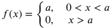
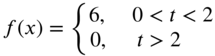
- 7.1 Find the Fourier transforms of the following functions:
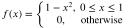
- 7.2 Find the Fourier cosine transforms of the following functions:
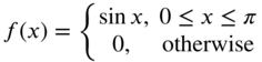
- 7.3 Find the Fourier sine transforms of the following functions:
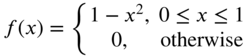
- 7.4 Find the Fourier cosine transforms of the following functions:
- 7.5 Find the Fourier sine transforms of the following functions:
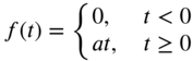
- 7.6 Find the Laplace transforms of the following functions:
- 7.7 Find the Laplace transforms of the following functions:
- 7.8 Find the Laplace transforms of the following functions:

- Heaviside's unit step function:

- 7.9 A single‐degree‐of‐freedom spring–mass–damper system is subjected to a displacement
 and velocity
  at time
  . Determine the resulting motion of the mass (m) using Laplace transforms. Assume the spring and damping forces to be kx and
  , where k is the spring constant and
  is the velocity of the mass, and the values of m, c and k as 1, 20 and 500, respectively.
 - 7.10 Derive an expression for the response of a uniform beam of length l fixed at both ends when subjected to a concentrated force
 at
at  . Assume the initial conditions of the beam to be zero. Use Fourier transforms.
 - 7.11 Find the response of a uniform beam of length l fixed at both the ends when subjected to an impulse
 at
at  . Assume that the beam is in equilibrium before the impulse is applied. Use Fourier transforms.
 - 7.12 A semi‐infinitely long string, along the x‐axis, is initially at rest. The string is subjected to a transverse displacement of
 at the end
  for
for  . Find the transverse displacement response of the string using Laplace transforms.
 - 7.13 Consider a finite string of length l fixed at
 and
and  , subjected to tension P. Find the transverse displacement of a string that is initially at rest and subjected to an impulse
  at point
  using the Fourier transform method.
 - 7.14 Find the steady‐state transverse vibration response of a string of length l fixed at both ends, subjected to the force

using the Fourier transform method.
- 7.15 Find the Laplace transforms of the following functions:
- 7.16 Find the solution of the following differential equation using Laplace transforms:
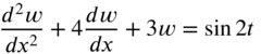
with
 and
and  .
. - 7.17 The longitudinal vibration of a uniform bar of length l is governed by the equation
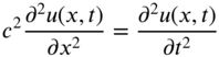
where
 with E and
  denoting Young's modulus and the mass density of the bar respectively. The bar is fixed at
  and free at
  . Find the free vibration response of the bar subject to the initial conditions
using Laplace transforms.
- 7.18 Find the longitudinal vibration response of a uniform bar fixed at
 and subjected to an axial force
  at
at  , using Laplace transforms. The equation of motion is given in Problem 7.17.
 - 7.19 A uniform bar fixed at
 , is subjected to a sudden displacement of magnitude
  at
at  . Find the ensuing axial motion of the bar using Laplace transforms. The governing equation of the bar is given in Problem 7.17.
 - 7.20 A taut string of length 1, fixed at
 and
and  is subjected to tension P. If the string is given an initial displacement
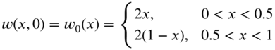
and released with zero velocity, determine the ensuing motion of the string.