
13
Vibration of Membranes
13.1 INTRODUCTION
A membrane is a perfectly flexible thin plate or lamina that is subjected to tension. It has negligible resistance to shear or bending forces, and the restoring forces arise exclusively from the in‐plane stretching or tensile forces. The drumhead and diaphragms of condenser microphones are examples of membranes.
13.2 EQUATION OF MOTION
13.2.1 Equilibrium Approach
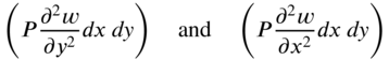
Consider a homogeneous and perfectly flexible membrane bounded by a plane curve C in the xy plane in the undeformed state. It is subjected to a pressure loading of intensity f(x, y, t) per unit area in the transverse or z direction and tension of magnitude P per unit length along the edge as in the case of a drumhead. Each point of the membrane is assumed to move only in the z direction, and the displacement, w(x, y, t), is assumed to be very small compared to the dimensions of the membrane. Consider an elemental area of the membrane, dx dy, with tensile forces of magnitude P dx and P dy acting on the sides parallel to the x and y axes, respectively, as shown in Fig. 13.1. After deformation, the net forces acting on the element of the membrane along the z direction due to the forces P dx and P dy will be (see Fig. 13.1(d))
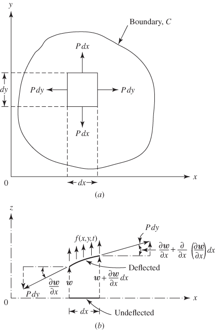

Figure 13.1 (a) Undeformed membrane in the xy plane; (b) deformed membrane as seen in the xz plane; (c) deformed membrane as seen in the yz plane; (d) forces acting on an element of the membrane.
The pressure force acting on the element of the membrane in the z direction is f(x, y) dx dy. The inertia force on the element is given by

where ![]() is the mass per unit area. The application of Newton's second law of motion yields the equation of motion for the forced transverse vibration of the membrane as
is the mass per unit area. The application of Newton's second law of motion yields the equation of motion for the forced transverse vibration of the membrane as

When the external force ![]() , the free vibration equation can be expressed as
, the free vibration equation can be expressed as

where
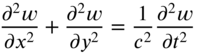
Equation (13.2) is also known as the two‐dimensional wave equation, with c denoting the wave velocity.
Initial and Boundary Conditions
Since the equation of motion, Eq. (13.1) or (13.2), involves second‐order partial derivatives with respect to each of t, x, and y, we need to specify two initial conditions and four boundary conditions to find a unique solution of the problem. Usually, the displacement and velocity of the membrane at ![]() are specified as
are specified as ![]() and
and ![]() , respectively. Thus, the initial conditions are given by
, respectively. Thus, the initial conditions are given by
The boundary conditions of the membrane can be stated as follows:
- If the membrane is fixed at any point
 on the boundary, the deflection must be zero, and hence
(13.6)
on the boundary, the deflection must be zero, and hence
(13.6)
- If the membrane is free to deflect transversely (in the z direction) at any point
 of the boundary, there cannot be any force at the point in the z direction. Thus,
(13.7)where
of the boundary, there cannot be any force at the point in the z direction. Thus,
(13.7)where
 indicates the derivative of w with respect to a direction n normal to the boundary at the point
  .
.
13.2.2 Variational Approach
To derive the equation of motion of a membrane using the extended Hamilton's principle, the expressions for the strain and kinetic energies as well as the work done by external forces are needed. The strain and kinetic energies of a membrane can be expressed as

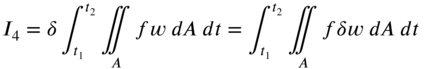
The work done by the distributed pressure loading f(x, y, t) is given by

The application of Hamilton's principle gives

or

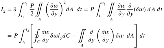
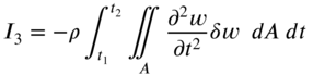
The variations in Eq. (13.12) can be evaluated using integration by parts as follows:

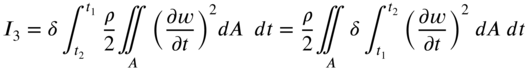
By using integration by parts with respect to time, the integral ![]() can be written as
can be written as

Since ![]() vanishes at
vanishes at ![]() and
and ![]() , Eq. (13.16) reduces to
, Eq. (13.16) reduces to
Using Eqs. (13.13), (13.14), (13.17), and (13.18), Eq. (13.12) can be expressed as

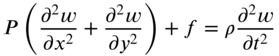
By setting each of the expressions under the brackets in Eq. (13.19) equal to zero, we obtain the differential equation of motion for the transverse vibration of the membrane as
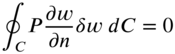
and the boundary condition as

Note that Eq. (13.21) will be satisfied for any combination of boundary conditions for a rectangular membrane. For a fixed edge:
For a free edge with ![]() or
or ![]() and
and ![]() :
:
With ![]() or
or ![]() ,
, ![]() and
and ![]() :
:

For arbitrary geometries of the membrane, Eq. (13.21) can be expressed as
which will be satisfied when either the edge is fixed with
or the edge is free with
13.3 WAVE SOLUTION
The functions
can be verified as the solutions of the two‐dimensional wave equation, Eq. (13.2). For example, consider the function ![]() given by Eq. (13.30). The partial derivatives of
given by Eq. (13.30). The partial derivatives of ![]() with respect to x, y, and t are given by
with respect to x, y, and t are given by


where a prime denotes a derivative with respect to the argument of the function. When ![]() is substituted for w using the relations (13.32), (13.34), and (13.36), Eq. (13.2) can be seen to be satisfied. The solutions given by Eqs. (13.28) and (13.29) are the same as those of a string. Equation (13.28) denotes a wave moving in the positive x direction at velocity c with its crests parallel to the y axis. The shape of the wave is independent of y and the membrane behaves as if it were made up of an infinite number of strips, all parallel to the x axis. Similarly, Eq. (13.29) denotes a wave moving in the negative x direction with crests parallel to the x axis and the shape independent of x. Equation (13.30) denotes a parallel wave moving in a direction at an angle
is substituted for w using the relations (13.32), (13.34), and (13.36), Eq. (13.2) can be seen to be satisfied. The solutions given by Eqs. (13.28) and (13.29) are the same as those of a string. Equation (13.28) denotes a wave moving in the positive x direction at velocity c with its crests parallel to the y axis. The shape of the wave is independent of y and the membrane behaves as if it were made up of an infinite number of strips, all parallel to the x axis. Similarly, Eq. (13.29) denotes a wave moving in the negative x direction with crests parallel to the x axis and the shape independent of x. Equation (13.30) denotes a parallel wave moving in a direction at an angle ![]() to the x axis with a velocity c.
to the x axis with a velocity c.
13.4 FREE VIBRATION OF RECTANGULAR MEMBRANES
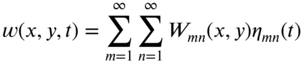
The free vibration of a rectangular membrane of sides a and b (Fig. 13.2) can be determined using the method of separation of variables. Thus, the displacement w(x, y, t) is expressed as a product of three functions as
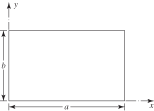
Figure 13.2 Rectangular membrane.
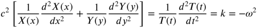
where W is a function of x and y, and X, Y, and T are functions of x, y, and t, respectively. Substituting Eq. (13.37) into the free vibration equation, Eq. (13.2), and dividing the resulting expression through by X(x)Y(y)T(t), we obtain

Since the left‐hand side of Eq. (13.38) is a function of x and y only, and the right‐hand side is a function of t only, each side must be equal to a constant, say, ![]() :
:
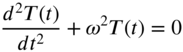
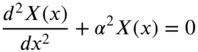
Equation (13.39) can be rewritten as two separate equations:

It can be noted, again, that the left‐hand side of Eq. (13.40) is a function of x only and the right‐hand side is a function of y only. Hence, Eq. (13.40) can be rewritten as two separate equations:

where ![]() and
and ![]() are new constants related to
are new constants related to ![]() as
as
Thus, the problem of solving a partial differential equation involving three variables, Eq. (13.2), has been reduced to the problem of solving three second‐order ordinary differential equations, Eqs. (13.41)–(13.43). The solutions of Eqs. (13.41)– (13.43) can be expressed as2
where the constants A and B can be determined from the initial conditions and the constants ![]() to
to ![]() can be found from the boundary conditions of the membrane.
can be found from the boundary conditions of the membrane.
13.4.1 Membrane with Clamped Boundaries
If a rectangular membrane is clamped or fixed on all the edges, the boundary conditions can be stated as
(13.50)
(13.51)

In view of Eq. (13.37), the boundary conditions of Eqs. (13.48)–(13.51) can be restated as
The conditions ![]() and
and ![]() (Eqs. [13.52] and [13.54]) require that
(Eqs. [13.52] and [13.54]) require that ![]() in Eq. (13.46) and
in Eq. (13.46) and ![]() in Eq. (13.47). Thus, the functions X(x) and Y(y) become
in Eq. (13.47). Thus, the functions X(x) and Y(y) become
For nontrivial solutions of X(x) and Y(y), the conditions ![]() and
and ![]() (Eqs. [13.53] and [13.55]) require that
(Eqs. [13.53] and [13.55]) require that
Equations (13.58) and (13.59) together define the eigenvalues of the membrane through Eq. (13.44). The roots of Eqs. (13.58) and (13.59) are given by
(13.61)
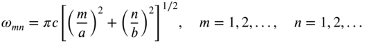
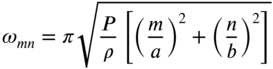
The natural frequencies of the membrane, ![]() , can be determined using Eq. (13.44) as
, can be determined using Eq. (13.44) as
or
The following observations can be made from Eq. (13.62):
- For any given mode of vibration, the natural frequency will decrease if either side of the rectangle is increased.
- The fundamental natural frequency,
 , is most influenced by changes in the shorter side of the rectangle.
 - For an elongated rectangular membrane (with
 ), the fundamental natural frequency,
  , is negligibly influenced by variations in the longer side.
The eigenfunction or mode shape, ![]() , of the membrane corresponding to the natural frequency
, of the membrane corresponding to the natural frequency ![]() is given by
is given by
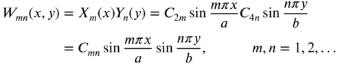
where ![]() is a constant. Thus, the natural mode of vibration corresponding to
is a constant. Thus, the natural mode of vibration corresponding to ![]() can be expressed as
can be expressed as
where ![]() and
and ![]() are new constants. The general solution of Eq. (13.64) is given by the sum of all the natural modes as
are new constants. The general solution of Eq. (13.64) is given by the sum of all the natural modes as

The constants ![]() and
and ![]() in Eq. (13.65) can be determined using the initial conditions stated in Eqs. (13.4) and (13.5). Substituting Eq. (13.65) into Eqs. (13.4) and (13.5), we obtain
in Eq. (13.65) can be determined using the initial conditions stated in Eqs. (13.4) and (13.5). Substituting Eq. (13.65) into Eqs. (13.4) and (13.5), we obtain

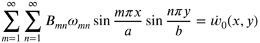
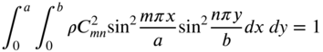
Equations (13.66) and (13.67) denote the double Fourier sine series expansions of the functions ![]() and
and ![]() , respectively. Multiplying Eqs. (13.66) and (13.67) by sin(mπx/a) sin(nπy/b) and integrating over the area of the membrane leads to the relations
, respectively. Multiplying Eqs. (13.66) and (13.67) by sin(mπx/a) sin(nπy/b) and integrating over the area of the membrane leads to the relations


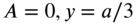
13.4.2 Mode Shapes
Equation (13.64) describes a possible displacement variation of a membrane clamped at the boundary. Each point of the membrane moves harmonically with circular frequency ![]() and amplitude given by the eigenfunction
and amplitude given by the eigenfunction ![]() of Eq. (13.63). The following observations can be made regarding the characteristics of mode shapes [8].
of Eq. (13.63). The following observations can be made regarding the characteristics of mode shapes [8].
- The fundamental or lowest mode shape of the membrane corresponds to
 . In this modal pattern, the deflected surface of the membrane will consist of one half of a sine wave in each of the x and y directions. The higher values of m and n correspond to mode shapes with m and n half sine waves along the x and y directions, respectively. Thus, for values of m and n greater than 1, the deflection (mode) shapes will consist of lines within the membrane along which the deflection is zero. The lines along which the deflection is zero during vibration are called nodal lines. For specificity, the nodal lines corresponding to
  are shown in Fig. 13.4. For example, for
  and
and  , the nodal line will be parallel to the y axis at
  , as shown in Fig. 13.5(a). Note that a specific natural frequency is associated with each combination of m and n values.
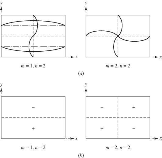
Figure 13.4 (a) modal patterns and nodal lines; (b) schematic illustration of mode shapes (+, positive deflection; −, negative deflection).

Figure 13.5 Modal patterns with
 and
and  .
. - Equation (13.62) indicates that some of the higher natural frequencies
 are integral multiples of the fundamental natural frequency
 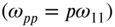 , where p is an integer, whereas some higher frequencies are not integral multiples of
  . For example,
  , and
, and  are not integral multiples of
  .
. - It can be seen that when
 and
and  are incommensurable, no two pairs of values of m and n can result in the same natural frequency. However, when
  and
and  are commensurable, two or more values of
  may have the same magnitude. If the ratio of sides
  is a rational number, the eigenvalues
  and
and  will have the same magnitude if
For example,
 , etc. when
  , and
, and  , etc. when
  .
. - If the membrane is square,
 and Eq. (13.70) reduces to
(13.71)and the magnitudes of
and Eq. (13.70) reduces to
(13.71)and the magnitudes of
 and
and  will be the same. This means that two different eigenfunctions
  and
and  correspond to the same frequency
  ; thus, there will be fewer frequencies than modes. Such cases are called degenerate cases. If the natural frequencies are repeated with
  , any linear combination of the corresponding natural modes
  and
and  can also be shown to be a natural mode of the membrane. Thus, for these cases, a large variety of nodal patterns occur.
 - To find the modal patterns and nodal lines of a square membrane corresponding to repeated frequencies, consider, as an example, the case of
 with
with  and
and  . For this case,
  and the corresponding distinct mode shapes can be expressed as (with
  )
)
Since the frequencies are the same, it will be of interest to consider a linear combination of the maximum deflection patterns given by Eqs. (13.72) and (13.73) as
where A and B are constants. The deflection shapes given by Eq. (13.74) for specific combinations of values of A and B are shown in Fig. 13.6. Figures 13.6(a)– 13.6(d) correspond to values of
 , and
, and  , respectively. When
  , the deflection shape given by Eq. (13.74) consists of one half sine wave along the x direction and two half sine waves along the y direction with a nodal line at
  . Similarly, when
  , the nodal line will be at
  . When
  , Eq. (13.74) becomes
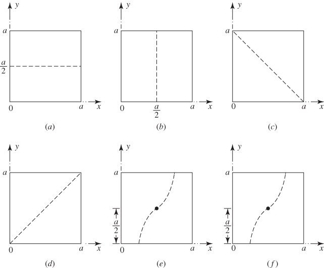
Figure 13.6 Deflection shapes given by Eq. (13.74): (a)
 ; (b)
; (b)  ; (c)
; (c)  ; (d)
; (d)  ; (e)
; (e)  ; (f)
; (f)  .
.It can be seen that
 in Eq. (13.75) when
or
The cases in Eq. (13.76) correspond to
 along the edges of the membrane, while the case in Eq. (13.77) gives
  at which
Equation (13.78) indicates that the nodal line is a diagonal of the square as shown in Fig. 13.6(c). Similarly, the case
 gives the nodal line along the other diagonal of the square as indicated in Fig. 13.6(d). For arbitrary values of A and B, Eq. (13.74) can be written as
where
 is a constant. Different nodal lines can be obtained based on the value of R. For example, the nodal line (along which
  in Eq. [13.79]) corresponding to
  is shown in Figs. 13.6(e) and (f).
The following observations can be made from the discussion above:
- A large variety of nodal patterns can exist for any repeated frequency in a square or rectangular membrane. Thus, it is not possible to associate a mode shape uniquely with a frequency in a membrane problem.
- The nodal lines need not be straight lines. It can be shown that all the nodal lines of a square membrane pass through the center,
 , which is called a pole.
- For a square membrane, the modal pattern corresponding to
 consists of one half of a sine wave along each of the x and y directions. For
  , no other pair of integers i and j give the same natural frequency,
  . In this case the maximum modal deflection can be expressed as
(13.80)
. In this case the maximum modal deflection can be expressed as
(13.80)
The nodal lines corresponding to this mode are determined by the equation
Equation (13.81) gives the nodal lines as (in addition to the edges)
(13.82)
which are shown in Fig. 13.7.

Figure 13.7 Nodal lines corresponding to
 of a square membrane.
 - Next, consider the case of
 and
and  for a square membrane. In this case,
  and the corresponding distinct mode shapes can be expressed as
Since the frequencies are the same, a linear combination of the maximum deflection patterns given by Eqs. (13.83) and (13.84) can be represented as
where A and B are constants. The nodal lines corresponding to Eq. (13.85) are defined by
 , which can be rewritten as
Neglecting the factor
 , which corresponds to nodal lines along the edges, Eq. (13.86) can be expressed as
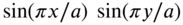
It can be seen from Eq. (13.87) that:
- When
 and 2a/3 denote the nodal lines.
 - When
 and 2a/3 denote the nodal lines.
 - When
 , Eq. (13.87) reduces to
(13.88)or
, Eq. (13.87) reduces to
(13.88)or (13.89)denote the nodal lines.
- When
 , Eq. (13.87) reduces to
(13.90)which represents a circle. The nodal lines in each of these cases are shown in Fig. 13.8.
, Eq. (13.87) reduces to
(13.90)which represents a circle. The nodal lines in each of these cases are shown in Fig. 13.8.
Figure 13.8 Nodal lines of a square membrane corresponding to
 : (a)
: (a)  ; (b)
; (b)  ; (c)
; (c)  ; (d)
; (d)  .
.
- When
- Whenever, in a vibrating system, including a membrane, certain parts or points remain at rest, they can be assumed to be absolutely fixed and the result may be applicable to another system. For example, at a particular natural frequency
 , if the modal pattern of a square membrane consists of a diagonal line as a nodal line, the solution will also be applicable for a membrane whose boundary is an isosceles right triangle. In addition, it can be observed that each possible mode of vibration of the isosceles triangle corresponds to some natural mode of the square. Accordingly, the fundamental natural frequency of vibration of an isosceles right triangle will be equal to the natural frequency of a square with
  and
and  :
:
The second natural frequency of the isosceles right triangle will be equal to the natural frequency of a square plate with
 and
and  :
:The mode shapes corresponding to the natural frequencies of Eqs. (13.91) and (13.92) are shown in Fig. 13.9.
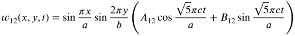


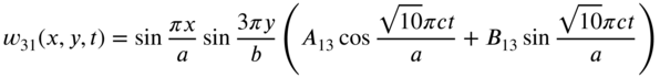

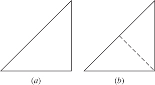
Figure 13.9 (a)  ; (b)
; (b)  .
.
13.5 FORCED VIBRATION OF RECTANGULAR MEMBRANES
13.5.1 Modal Analysis Approach
The equation of motion governing the forced vibration of a rectangular membrane is given by Eq. (13.1):

We can find the solution of Eq. (13.93) using the modal analysis procedure. Accordingly, we assume the solution of Eq. (13.93) as
where ![]() are the natural modes of vibration and
are the natural modes of vibration and ![]() are the corresponding generalized coordinates. For specificity, we consider a membrane with clamped edges. For this, the eigenfunctions are given by Eq. (13.63):
are the corresponding generalized coordinates. For specificity, we consider a membrane with clamped edges. For this, the eigenfunctions are given by Eq. (13.63):
The eigenfunctions (or normal modes) can be normalized as

or
The simplification of Eq. (13.97) yields

Thus, the normal modes take the form

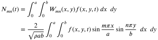
Substituting Eq. (13.94) into Eq. (13.93), multiplying the resulting equation throughout by ![]() , and integrating over the area of the membrane leads to the equation
, and integrating over the area of the membrane leads to the equation
where
The solution of Eq. (13.100) can be written as (see Eq. [2.109])

The solution of Eq. (13.93) becomes, in view of Eqs. (13.94) and (13.103),
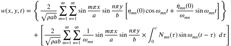
It can be seen that the quantity inside the braces represents the free vibration response (due to the initial conditions) and the quantity in the second set of brackets denotes the forced vibrations of the membrane.
13.5.2 Fourier Transform Approach
The governing equation can be expressed as (see Eqs. [13.1]–[13.3])

where w(x, y, t) is the transverse displacement. Let the membrane be fixed along all the edges, ![]() , and
, and ![]() . Multiplying Eq. (13.105) by
. Multiplying Eq. (13.105) by ![]() and integrating the resulting equation over the area of the membrane yields
and integrating the resulting equation over the area of the membrane yields

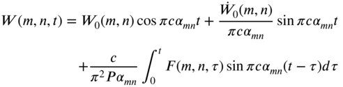
where W(m, n, t) and F(m, n, t) denote the double finite Fourier sine transforms of w(x, y, t) and f(x, y, t), respectively:


The solution of Eq. (13.106) can be expressed as
where ![]() and
and ![]() are the double finite Fourier sine transforms of the initial values of w and
are the double finite Fourier sine transforms of the initial values of w and ![]() :
:


where

The displacement of the membrane can be found by taking the double inverse finite sine transform of Eq. (13.109). The procedure is illustrated for a simple case in Example 13.3.
13.6 FREE VIBRATION OF CIRCULAR MEMBRANES
13.6.1 Equation of Motion
Noting that the Laplacian operator in rectangular coordinates is defined by

the equation of motion of a rectangular membrane, Eq. (13.1), can be expressed for free vibration as

For a circular membrane, the governing equation of motion can be derived using an equilibrium approach by considering a differential element in the polar coordinates r and ![]() (see Problem 13.1). Alternatively, a coordinate transformation using the relations
(see Problem 13.1). Alternatively, a coordinate transformation using the relations
can be used to express the Laplacian operator in polar coordinates as (see Problem 13.2)

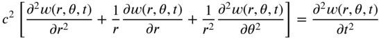
Thus, the equation of motion for the free vibration of a circular membrane can be expressed as

which can be rewritten as
where ![]() as given by Eq. (13.3). As the displacement, w, is now a function of r,
as given by Eq. (13.3). As the displacement, w, is now a function of r, ![]() , and t, we use the method of separation of variables and express the solution as
, and t, we use the method of separation of variables and express the solution as
where R, ![]() , and T are functions of only r,
, and T are functions of only r, ![]() , and t, respectively. By substituting Eq. (13.121) into Eq. (13.120), we obtain
, and t, respectively. By substituting Eq. (13.121) into Eq. (13.120), we obtain
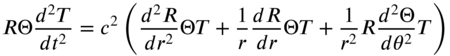
which, upon division by ![]() , becomes
, becomes

Noting that each side of Eq. (13.123) must be a constant with a negative value (see Problem 13.3), the constant is taken as ![]() , where
, where ![]() is any number, and Eq. (13.123) is rewritten as
is any number, and Eq. (13.123) is rewritten as
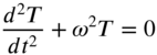

Again, we note that each side of Eq. (13.125) must be a positive constant. Using ![]() as the constant, Eq. (13.125) is rewritten as
as the constant, Eq. (13.125) is rewritten as


Since the constant ![]() must yield the displacement w as a periodic function of
must yield the displacement w as a periodic function of ![]() with a period
with a period ![]() (i.e.
(i.e. ![]() ),
), ![]() must be an integer:
must be an integer:
The solutions of Eqs. (13.124) and (13.127) can be expressed as
By defining ![]() , Eq. (13.126) can be rewritten as
, Eq. (13.126) can be rewritten as
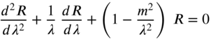
which can be identified as Bessel's differential equation of order m whose solution can be expressed as [9]
where ![]() and
and ![]() are constants to be determined from the boundary conditions, and
are constants to be determined from the boundary conditions, and ![]() and
and ![]() are called Bessel functions of order m and of the first and second kind, respectively. The Bessel functions are in the form of infinite series and are studied extensively and tabulated in the literature [2], [3] because of their importance in the study of problems involving circular geometry. For a circular membrane,
are called Bessel functions of order m and of the first and second kind, respectively. The Bessel functions are in the form of infinite series and are studied extensively and tabulated in the literature [2], [3] because of their importance in the study of problems involving circular geometry. For a circular membrane, ![]() must be finite (bounded) everywhere. However,
must be finite (bounded) everywhere. However, ![]() approaches infinity at the origin
approaches infinity at the origin ![]() . Hence, the constant
. Hence, the constant ![]() must be zero in Eq. (13.132). Thus, Eq. (13.132) reduces to
must be zero in Eq. (13.132). Thus, Eq. (13.132) reduces to
Thus, the complete solution can be expressed as
where
with ![]() and
and ![]() denoting some new constants.
denoting some new constants.
13.6.2 Membrane with a Clamped Boundary
If the membrane is clamped or fixed at the boundary ![]() , the boundary conditions can be stated as
, the boundary conditions can be stated as
Using Eq. (13.136), Eq. (13.135) can be expressed as
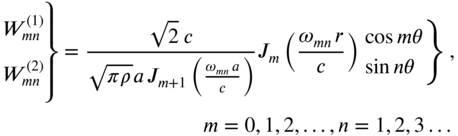
The Bessel function of the first kind, ![]() , is given by [2], [3]
, is given by [2], [3]

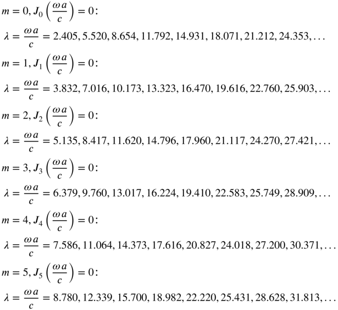
Equation (13.137) has to be satisfied for all values of θ. It can be satisfied only if
This is the frequency equation, which has an infinite number of discrete solutions, ![]() for each value of m. Although
for each value of m. Although ![]() is a root of Eq. (13.139) for
is a root of Eq. (13.139) for ![]() , this leads to the trivial solutions
, this leads to the trivial solutions ![]() , and hence we need to consider roots with
, and hence we need to consider roots with ![]() . Some of the roots of Eq. (13.139) are given below [2], [3]. For
. Some of the roots of Eq. (13.139) are given below [2], [3]. For ![]() ,
, ![]() :
:
It can be seen from Eqs. (13.134) and (13.135) that the general solution of ![]() becomes complicated in view of the various combinations of
becomes complicated in view of the various combinations of ![]() , and
, and ![]() involved for each value of
involved for each value of ![]() Hence, the solution is usually expressed in terms of two characteristic functions
Hence, the solution is usually expressed in terms of two characteristic functions ![]() and
and ![]() as indicated below. If
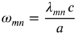
as indicated below. If ![]() denotes the nth solution or root of
denotes the nth solution or root of ![]() , the natural frequencies can be expressed as
, the natural frequencies can be expressed as
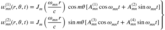
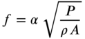
Two characteristic functions ![]() and
and ![]() can be defined for any
can be defined for any ![]() as
as

It can be seen that for any given values of m and ![]() the two characteristic functions will have the same shape; they differ from one another only by an angular rotation of 90°. Thus, the two natural modes of vibration corresponding to
the two characteristic functions will have the same shape; they differ from one another only by an angular rotation of 90°. Thus, the two natural modes of vibration corresponding to ![]() are given by
are given by
The general solution of Eq. (13.120) can be expressed as
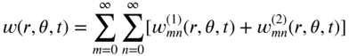
where the constants ![]() can be determined from the initial conditions.
can be determined from the initial conditions.
13.6.3 Mode Shapes
It can be seen from Eq. (13.141) that the characteristic functions or normal modes will have the same shape for any given values of m and n, and differ from one another only by an angular rotation of 90°. In the mode shapes given by Eq. (13.141), the value of m determines the number of nodal diameters. The value of n, indicating the order of the root or the zero of the Bessel function, denotes the number of nodal circles in the mode shapes. The nodal diameters and nodal circles corresponding to ![]() , and 2 are shown in Fig. 13.11. When
, and 2 are shown in Fig. 13.11. When ![]() , there will be no diametrical nodal lines but there will be n circular nodal lines, including the boundary of the membrane. When
, there will be no diametrical nodal lines but there will be n circular nodal lines, including the boundary of the membrane. When ![]() , there will be one diametrical node and n circular nodes, including the boundary. In general, the mode shape
, there will be one diametrical node and n circular nodes, including the boundary. In general, the mode shape ![]() has m equally spaced diametrical nodes and n circular nodes (including the boundary) of radius
has m equally spaced diametrical nodes and n circular nodes (including the boundary) of radius ![]() . The mode shapes corresponding to a few combinations of m and n are shown in Fig. 13.11.
. The mode shapes corresponding to a few combinations of m and n are shown in Fig. 13.11.
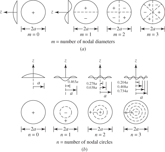
Figure 13.11 Mode shapes of a clamped circular membrane.
13.7 FORCED VIBRATION OF CIRCULAR MEMBRANES
The equation of motion governing the forced vibration of a circular membrane is given by Eq. (13.119):

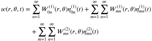
Using modal analysis, the solution of Eq. (13.144) is assumed in the form

where ![]() are the natural modes of vibration and
are the natural modes of vibration and ![]() are the corresponding generalized coordinates. For specificity, we consider a circular membrane clamped at the edge,
are the corresponding generalized coordinates. For specificity, we consider a circular membrane clamped at the edge, ![]() . For this, the eigenfunctions are given by Eq. (13.141), since two eigenfunctions are used for any
. For this, the eigenfunctions are given by Eq. (13.141), since two eigenfunctions are used for any ![]() , the modes will be degenerate except when
, the modes will be degenerate except when ![]() , and we rewrite Eq. (13.145) as
, and we rewrite Eq. (13.145) as
where the normal modes ![]() ,
, ![]() and
and ![]() are given by Eq. (13.141). The normal modes can be normalized as
are given by Eq. (13.141). The normal modes can be normalized as
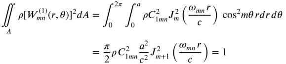
where A is the area of the circular membrane. Equation (147) yields


or
Thus, the normalized normal modes can be expressed as
When Eq. (13.145) is used, Eq. (13.144) yields the equations
where ![]() denotes the generalized force given by
denotes the generalized force given by

Neglecting the contribution due to initial conditions, the generalized coordinates can be expressed as (see Eq. [2.109])


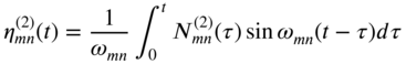
where the natural frequencies ![]() are given by Eq. (13.140), and the generalized forces by Eq. (13.153).
are given by Eq. (13.140), and the generalized forces by Eq. (13.153).
13.8 MEMBRANES WITH IRREGULAR SHAPES
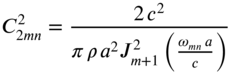
The known natural frequencies of vibration of rectangular and circular membranes can be used to estimate the natural frequencies of membranes having irregular boundaries. For example, the natural frequencies of a regular polygon are expected to lie in between those of the inscribed and circumscribed circles. Rayleigh presented an analysis to find the effect of a departure from the exact circular shape on the natural frequencies of vibration of uniform membranes. The results of the analysis indicate that for membranes of fairly regular shape, the fundamental or lowest natural frequency of vibration can be approximated as
where P is the tension, ![]() is the density per unit area, A is the surface area, and
is the density per unit area, A is the surface area, and ![]() is a factor whose values are given in Table 13.1 for several irregular shapes. The factors given in Table 13.1 indicate, for instance, that for the same values of tension, density, and surface area, the fundamental natural frequency of vibration of a square membrane is larger than that of a circular membrane by the factor
is a factor whose values are given in Table 13.1 for several irregular shapes. The factors given in Table 13.1 indicate, for instance, that for the same values of tension, density, and surface area, the fundamental natural frequency of vibration of a square membrane is larger than that of a circular membrane by the factor ![]() .
.
Table 13.1 Values of the factor α in Eq. (13.157).
| Shape of the membrane | |
| Square | 4.443 |
| Rectangle with |
4.967 |
| Rectangle with |
5.736 |
| Rectangle with |
4.624 |
| Circle | 4.261 |
| Semicircle | 4.803 |
| Quarter circle | 4.551 |
| 60° sector of a circle | 4.616 |
| Equilateral triangle | 4.774 |
| Isosceles right triangle | 4.967 |
Source: Ref. [8].
13.9 PARTIAL CIRCULAR MEMBRANES
Consider a membrane in the form of a circular sector of radius a as shown in Fig. 13.13. Let the membrane be fixed on all three edges. When the zero‐displacement conditions along the edges ![]() and
and ![]() are used in the general solution of Eq. (13.134), we find that the solution becomes
are used in the general solution of Eq. (13.134), we find that the solution becomes
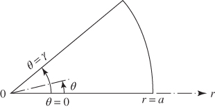
Figure 13.13 Circular sector membrane.
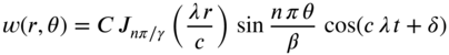
where C is a constant and n is an integer. To satisfy the boundary condition along the edge ![]() , Eq. (13.158) is set equal to zero at
, Eq. (13.158) is set equal to zero at ![]() . This leads to the frequency equation
. This leads to the frequency equation
If ![]() denotes the ith root of Eq. (13.159), the corresponding natural frequency of vibration can be computed as
denotes the ith root of Eq. (13.159), the corresponding natural frequency of vibration can be computed as

For example, for a semicircular membrane, ![]() and for
and for ![]() , Eq. (13.159) becomes
, Eq. (13.159) becomes
whose roots are given by ![]() , and
, and ![]() ,…. Thus, the natural frequencies of vibration of the semicircular membrane will be
,…. Thus, the natural frequencies of vibration of the semicircular membrane will be ![]() ….
….
13.10 RECENT CONTRIBUTIONS
Spence and Horgan [11] derived bounds on the natural frequencies of composite circular membranes using an integral equation method. The membrane was assumed to have a stepped radial density. Although such problems, involving discontinuous coefficients in the differential equation, can be treated using the classical variational methods, it was shown that an eigenvalue estimation technique based on an integral formulation is more efficient. For a comparable amount of effort, the integral equation method is expected to provide more accurate bounds on the natural frequencies.
The transient response of hanging curtains clamped at three edges was considered by Yamada et al. [12]. A hanging curtain was replaced by an equivalent membrane for deriving the equation of motion. The free vibration of the membrane was analyzed theoretically and its transient response when subjected to a rectangularly varying point force was also studied using Galerkin's method. The forced vibration response of a uniform membrane of arbitrary shape under an arbitrary distribution of time‐dependent excitation with arbitrary initial conditions and time‐dependent boundary conditions was found by Olcer [13]. Leissa and Ghamat‐Rezaei [14] presented the vibration frequencies and mode shapes of rectangular membranes subjected to shear stresses and/or nonuniform tensile stresses. The solution is found using the Ritz method, with the transverse displacement in the form of a double series of trigonometric functions.
The scalar wave equation of an annular membrane in which the motion is symmetrical about the origin was solved for arbitrary initial and boundary conditions by Sharp [15]. The solution was obtained using a finite Hankel transform. A simple example was given and its solution was compared with one given by the method of separation of variables. The vibration of a loaded kettledrum was considered by De [16]. In this work, the author discussed the effect of the applied mass load at a point on the frequency of a vibrating kettledrum. In a method of obtaining approximations of the natural frequencies of membranes developed by Torvik and Eastep [17], an approximate expression for the radius of the bounding curve is first written as a truncated Fourier series. The deflection, expressed as a superposition of the modes of the circular membrane, is forced to vanish approximately on the approximated boundary. This leads to a system of linear homogeneous equations in terms of the amplitudes of the modes of the circular membrane. By equating the determinant of coefficients to zero, the approximate frequencies are found. Some exact solutions of the vibration of nonhomogeneous membranes were presented by Wang [18], including the exact solutions of a rectangular membrane with a linear density variation and a nonhomogeneous annular membrane with inverse square density distribution.
NOTES
- The constant k can be shown to be a negative quantity by proceeding as in the case of free vibration of strings (Problem 13.3). Thus, we can write
 , where
  is another constant.
 - The solution given by Eqs. (13.45)– (13.47) can also be obtained by proceeding as follows. The equation governing the free vibration of a rectangular membrane can be expressed, setting
 in Eq. (13.1), as
By assuming a harmonic solution at frequency
 as(b)
as(b)
Eq. (a) can be expressed as
(c)
By assuming the solution of W(x, y) in the form
(d)
and proceeding as indicated earlier, the solution shown in Eqs. (13.45)– (13.47) can be obtained.
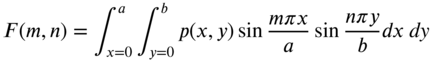
- If p(x, y) denotes a function of the variables x and y that satisfies the Dirichlet's condition over the region
 , its finite double Fourier sine transform, P(m, n), is defined by
The inverse transform of F(m, n), given by Eq. (a), can be expressed as
(b)
REFERENCES
- 1 K.F. Graff, Wave Motion in Elastic Solids, Ohio State University Press, Columbus, OH, 1975.
- 2 N.W. McLachlan, Bessel Functions for Engineers, Oxford University Press, New York, 1934.
- 3 G.N. Watson, Theory of Bessel Functions, Cambridge University Press, London, 1922.
- 4 L. Meirovitch, Analytical Methods in Vibrations, Macmillan, New York, 1967.
- 5 S. Timoshenko, D.H. Young, and W. Weaver, Jr., Vibration Problems in Engineering, 4th ed., Wiley, New York, 1974.
- 6 E. Volterra and E.C. Zachmanoglou, Dynamics of Vibrations, Charles E. Merrill, Columbus, OH, 1965.
- 7 S.K. Clark, Dynamics of Continuous Elements, Prentice‐Hall, Englewood Cliffs, NJ, 1972.
- 8 Lord Rayleigh, The Theory of Sound, 2nd ed., Vol. 1, Dover, New York, 1945.
- 9 A. Jeffrey, Advanced Engineering Mathematics, Harcourt/Academic Press, San Diego, CA, 2002.
- 10 P.M. Morse, Vibration and Sound, McGraw‐Hill, New York, 1936.
- 11 J.P. Spence and C.O. Horgan, Bounds on natural frequencies of composite circular membranes: integral equation methods, Journal of Sound and Vibration, Vol. 87, No. 1, pp. 71–81, 1983.
- 12 G. Yamada, Y. Kobayashi, and H. Hamaya, Transient response of a hanging curtain, Journal of Sound and Vibration, Vol. 130, No. 2, pp. 223–235, 1989.
- 13 N.Y. Olcer, General solution to the equation of the vibrating membrane, Journal of Sound and Vibration, Vol. 6, No. 3, pp. 365–374, 1967.
- 14 A.W. Leissa and A. Ghamat‐Rezaei, Vibrations of rectangular membranes subjected to shear and nonuniform tensile stresses, Journal of the Acoustical Society of America, Vol. 88, No. 1, pp. 231–238, 1990.
- 15 G.R. Sharp, Finite transform solution of the symmetrically vibrating annular membrane, Journal of Sound and Vibration, Vol. 5, No. 1, pp. 1–8, 1967.
- 16 S. De, Vibrations of a loaded kettledrum, Journal of Sound and Vibration, Vol. 20, No. 1, pp. 79–92, 1972.
- 17 P.J. Torvik and F.E. Eastep, A method for improving the estimation of membrane frequencies, Journal of Sound and Vibration, Vol. 21, No. 3, pp. 285–294, 1972.
- 18 C.Y. Wang, Some exact solutions of the vibration of non‐homogeneous membranes, Journal of Sound and Vibration, Vol. 210, No. 4, pp. 555–558, 1998.
PROBLEMS
- 13.1 Starting from the free‐body diagram of an element of a membrane in polar coordinates, derive the equation of motion of a vibrating membrane in polar coordinates using the equilibrium approach.
- 13.2 Derive the expression for the Laplacian operator in polar coordinates starting from the relation
and using the coordinate transformation relations
 and
and  .
. - 13.3 Show that each side of Eqs. (13.38) and (13.123) is equal to a negative constant.
- 13.4 Consider a rectangular membrane with the ratio of sides a and b equal to
 and all boundaries clamped. Find the distinct natural frequencies
  and
and  that will have the same magnitude.
 - 13.5 Find the forced vibration response of a rectangular membrane of sides a and b subjected to a suddenly applied uniformly distributed pressure
 per unit area. Assume zero initial conditions and the membrane to be fixed around all the edges.
 - 13.6 Find the steady‐state response of a rectangular membrane of sides a and b subjected to a harmonic force
 at the point
  . Assume the membrane to be clamped on all four edges.
 - 13.7 Derive the equation of motion of a membrane in polar coordinates using a variational approach.
- 13.8 A thin sheet of steel of thickness 0.01 mm is stretched over a rectangular metal framework of size 25 mm × 50 mm under a tension of 2 kN per unit length of periphery. Determine the first three natural frequencies of vibration and the corresponding mode shapes of the sheet. Assume the density of steel sheet to be
 .
. - 13.9 Solve Problem 13.8 by assuming the sheet to be aluminum instead of steel, with a density of
 .
. - 13.10 A thin sheet of steel of thickness 0.01 mm is stretched over a circular metal framework of diameter 50 mm under a tension of 2 kN per unit length of periphery. Determine the first three natural frequencies of vibration and the corresponding mode shapes of symmetric vibration of the sheet. Assume the density of the steel sheet to be
 .
. - 13.11 Solve Problem 13.10 by assuming the sheet to be aluminum instead of steel, with a density of
 .
. - 13.12 Derive the frequency equation of an annular membrane of inner radius
 and outer radius
  fixed at both edges.
 - 13.13 Find the free vibration response of a rectangular membrane of sides a and b subjected to the following initial conditions:

Assume that the membrane is fixed on all the sides.
- 13.14 Find the free vibration response of a rectangular membrane of sides a and b subjected to the following initial conditions:
Assume that the membrane is fixed on all sides.
- 13.15 Find the steady‐state response of a rectangular membrane fixed on all sides subjected to the force
 sin
sin  .
. - 13.16 Find the free vibration response of a circular membrane of radius a subjected to the following initial conditions:
Assume that the membrane is fixed at the outer edge,
 .
. - 13.17 Find the response of a rectangular membrane of sides a and b fixed on all four sides when subjected to an impulse
 at
at  .
. - 13.18 Find the steady‐state response of a circular membrane of radius a when subjected to the force
 at
at  .
. - 13.19 Derive the frequency equation of an annular membrane of inner radius b and outer radius a assuming a clamped inner edge and free outer edge.
- 13.20 Derive the frequency equation of an annular membrane of inner radius b and outer radius a assuming that it is free at both the inner and outer edges.