10
Torsional Vibration of Shafts
10.1 INTRODUCTION
Many rotating shafts and axles used for power transmission experience torsional vibration, particularly when the prime mover is a reciprocating engine. The shafts used in high‐speed machinery, especially those carrying heavy wheels, are subjected to dynamic torsional forces and vibration. A solid or hollow cylindrical rod of circular section undergoes torsional displacement or twisting such that each transverse section remains in its own plane when a torsional moment is applied. In this case the cross‐sections of the rod do not experience any motion parallel to the axis of the rod. However, if the cross‐section of the rod is not circular, the effect of a twist will be more involved. In this case the twist will be accompanied by a warping of normal cross‐sections. The torsional vibrations of uniform and nonuniform rods with circular cross‐section and rods with noncircular section are considered in this chapter. For noncircular sections, the equations of motion are derived using both the Saint‐Venant and the Timoshenko–Gere theories. The methods of determining the torsional rigidity of noncircular rods are presented using the Prandtl stress function and the Prandtl membrane analogy.
10.2 ELEMENTARY THEORY: EQUATION OF MOTION
10.2.1 Equilibrium Approach
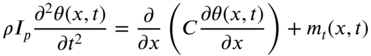
Consider an element of a nonuniform circular shaft between two cross‐sections at x and ![]() , as shown in Fig. 10.1(a). Let
, as shown in Fig. 10.1(a). Let ![]() denote the torque induced in the shaft at x and time t and
denote the torque induced in the shaft at x and time t and ![]() the torque induced in the shaft at
the torque induced in the shaft at ![]() and at the same time t. If the angular displacement of the cross‐section at x is denoted as
and at the same time t. If the angular displacement of the cross‐section at x is denoted as ![]() , the angular displacement of the cross‐section at
, the angular displacement of the cross‐section at ![]() can be represented as
can be represented as ![]() . Let the external torque acting on the shaft per unit length be denoted
. Let the external torque acting on the shaft per unit length be denoted ![]() . The inertia torque acting on the element of the shaft is given by
. The inertia torque acting on the element of the shaft is given by ![]() , where
, where ![]() is the mass polar moment of inertia of the shaft per unit length. Noting that
is the mass polar moment of inertia of the shaft per unit length. Noting that ![]() and
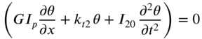
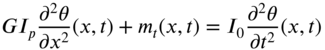
and ![]() , Newton's second law of motion can be applied to the element of the shaft to obtain the equation of motion as
, Newton's second law of motion can be applied to the element of the shaft to obtain the equation of motion as
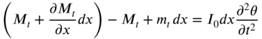

Figure 10.1 Torsional vibration of a nonuniform shaft.
From the strength of materials, the relationship between the torque in the shaft and the angular displacement is given by [1]
where G is the shear modulus and ![]() is the polar moment of inertia of the cross‐section of the shaft. Using Eq. (10.2), the equation of motion, Eq. (10.1), can be expressed as
is the polar moment of inertia of the cross‐section of the shaft. Using Eq. (10.2), the equation of motion, Eq. (10.1), can be expressed as

10.2.2 Variational Approach
The equation of motion of a nonuniform shaft, using the variational approach, has been derived in Section 4.11.1. In this section the variational approach is used to derive the equation of motion and the boundary conditions for a nonuniform shaft with torsional springs (with stiffnesses ![]() and
and ![]() ) and masses (with mass moments of inertia
) and masses (with mass moments of inertia ![]() and
and ![]() ) attached at each end as shown in Fig. 10.1.
) attached at each end as shown in Fig. 10.1.
The cross‐sections of the shaft are assumed to remain plane before and after angular deformation. Since the cross‐section of the shaft at x undergoes an angular displacement ![]() about the center of twist, the shape of the cross‐section does not change. The cross‐section simply rotates about the x axis. A typical point P rotates around the x axis by a small angle
about the center of twist, the shape of the cross‐section does not change. The cross‐section simply rotates about the x axis. A typical point P rotates around the x axis by a small angle ![]() as shown in Fig. 10.2. The displacements of point P parallel to the y and z axes are given by the projections of the displacement PP′ on oy and oz:
as shown in Fig. 10.2. The displacements of point P parallel to the y and z axes are given by the projections of the displacement PP′ on oy and oz:

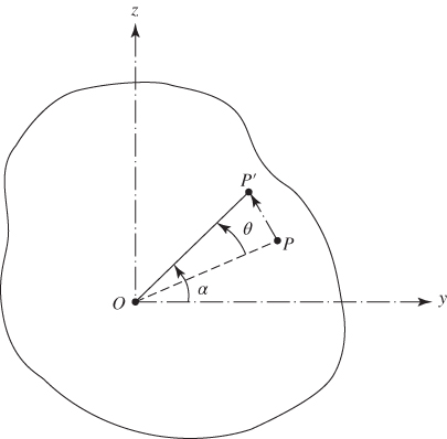
Figure 10.2 Rotation of a point in the cross‐section of a shaft.
Since ![]() is small, we can write
is small, we can write

so that
Thus, the displacement components of the shaft parallel to the three coordinate axes can be expressed as

The strains in the shaft are assumed to be

and the corresponding stresses are given by

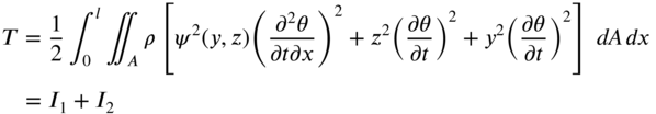
The strain energy of the shaft and the torsional springs is given by
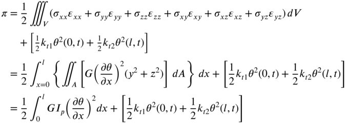
where  . The kinetic energy of the shaft can be expressed as

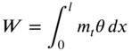
The work done by the external torque ![]() can be represented as
can be represented as
The application of the generalized Hamilton's principle yields

or

The variations in Eq. (10.13) can be evaluated using integration by parts to obtain


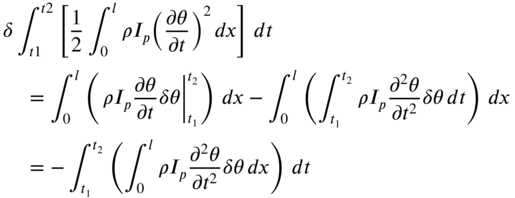

Note that integration by parts with respect to time, along with the fact that ![]() at
at ![]() and
and ![]() , has been used in deriving Eqs. (10.16) and (10.17). By using Eqs. (10.14)– (10.17) in Eq. (10.13), we obtain
, has been used in deriving Eqs. (10.16) and (10.17). By using Eqs. (10.14)– (10.17) in Eq. (10.13), we obtain
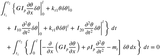
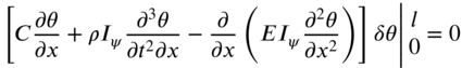
By setting the two expressions under the braces in each term of Eq. (10.18) equal to zero, we obtain the equation of motion for the torsional vibration of the shaft as

where ![]() is the mass moment of inertia of the shaft per unit length, and the boundary conditions as
is the mass moment of inertia of the shaft per unit length, and the boundary conditions as

Each of the equations in (10.20) can be satisfied in two ways but will be satisfied only one way for any specific end conditions of the shaft. The boundary conditions implied by Eqs. (10.20) are as follows. At ![]() , either
, either ![]() is specified (so that
is specified (so that ![]() ) or
) or
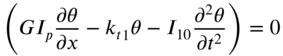
At ![]() , either
, either ![]() is specified (so that
is specified (so that ![]() ) or
) or
In the present case, the second conditions stated in each of Eqs. (10.21) and (10.22) are valid.
10.3 FREE VIBRATION OF UNIFORM SHAFTS
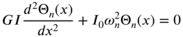
For a uniform shaft, Eq. (10.19) reduces to

By setting ![]() , we obtain the free vibration equation
, we obtain the free vibration equation
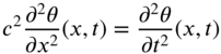
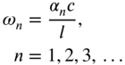
where
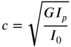
It can be observed that Eqs. (10.23)–(10.25) are similar to the equations derived in the cases of transverse vibration of a string and longitudinal vibration of a bar. For a uniform shaft, ![]() and Eq. (10.25) takes the form
and Eq. (10.25) takes the form

By assuming the solution as
Eq. (10.24) can be written as two separate equations:

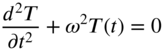
The solutions of Eqs. (10.28) and (10.29) can be expressed as
where A, B, C, and D are constants. If ![]() denotes the nth frequency of vibration and
denotes the nth frequency of vibration and ![]() the corresponding mode shape, the general free vibration solution of Eq. (10.24) is given by
the corresponding mode shape, the general free vibration solution of Eq. (10.24) is given by

The constraints ![]() and
and ![]() can be evaluated from the initial conditions, and the constraints
can be evaluated from the initial conditions, and the constraints ![]() and
and ![]() can be determined (not the absolute values, only their relative values) from the boundary conditions of the shaft. The initial conditions are usually stated in terms of the initial angular displacement and angular velocity distributions of the shaft.
can be determined (not the absolute values, only their relative values) from the boundary conditions of the shaft. The initial conditions are usually stated in terms of the initial angular displacement and angular velocity distributions of the shaft.
10.3.1 Natural Frequencies of a Shaft with Both Ends Fixed
For a uniform circular shaft of length l fixed at both ends, the boundary conditions are given by
The free vibration solution is given by Eq. (10.27):
Equations (10.33) and (10.35) yield
and the solution can be expressed as
where C′ and D′ are new constants. The use of Eq. (10.34) in (10.37) gives the frequency equation
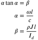
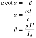
The natural frequencies of vibration are given by the roots of Eq. (10.38) as
or
The mode shape corresponding to the natural frequency ![]() can be expressed as
can be expressed as
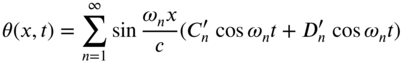
The free vibration solution of the fixed–fixed shaft is given by a linear combination of its normal modes:
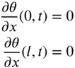
10.3.2 Natural Frequencies of a Shaft with Both Ends Free
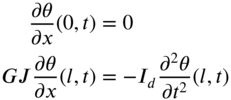
Since the torque, ![]() , is zero at a free end, the boundary conditions of a free–free shaft are given by
, is zero at a free end, the boundary conditions of a free–free shaft are given by
In view of Eq. (10.27), Eqs. (10.42) and (10.43) can be expressed as
Eq. (10.30) gives
Eqs. (10.44) and (10.47) yield
and Eqs. (10.45) and (10.47) result in
The roots of Eq. (10.49) are given by

The nth normal mode is given by
The free vibration solution of the shaft can be expressed as (see Eq. [10.32])

where the constants ![]() and
and ![]() can be determined from the initial conditions of the shaft.
can be determined from the initial conditions of the shaft.
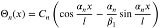
10.3.3 Natural Frequencies of a Shaft Fixed at One End and Attached to a Torsional Spring at the Other
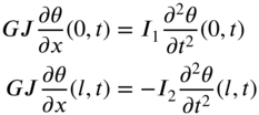
For a uniform circular shaft fixed at ![]() and attached to a torsional spring of stiffness
and attached to a torsional spring of stiffness ![]() at
at ![]() , as shown in Fig. 10.3, the boundary conditions are given by
, as shown in Fig. 10.3, the boundary conditions are given by
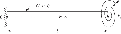
Figure 10.3 Shaft fixed at  and a torsional spring attached at
  .
.
The free vibration solution of a shaft is given by Eq. (10.27):
The use of the boundary condition of Eq. (10.53) in Eq. (10.55) gives
and the solution can be expressed as
The use of the boundary condition of Eq. (10.54) in Eq. (10.57) yields the frequency equation

Using Eq. (10.26), Eq. (10.58) can be rewritten as
where

The roots of the frequency equation (10.60) give the natural frequencies of vibration of the shaft as
and the corresponding mode shapes as
Finally, the free vibration solution of the shaft can be expressed as

Several possible boundary conditions for the torsional vibration of a uniform shaft are given in Table 10.1, along with the corresponding frequency equations and the mode shapes.
Table 10.1 Boundary conditions of a uniform shaft in torsional vibration.
| End conditions of shaft | Boundary conditions | Frequency equation | Mode shape (normal function) | Natural frequencies |
1. Fixed–free |
 |
 |
||
2. Free–free |
 |
 |
||
3. Fixed–fixed |
 |
 |
||
4. Fixed–disk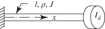 |
 |
 |
 |
|
5. Fixed–torsional spring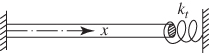 |
 |
 |
 |
|
6. Free–disk |
 |
 |
 |
|
7. Free–torsional spring |
 |
 |
 |
|
8. Disk–disk |
 |
 |
 |
 |
10.4 FREE VIBRATION RESPONSE DUE TO INITIAL CONDITIONS: MODAL ANALYSIS
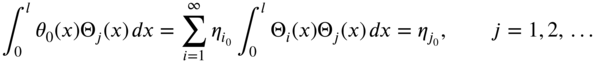
The angular displacement of a shaft in torsional vibration can be expressed in terms of normal modes ![]() using the expansion theorem, as
using the expansion theorem, as
where ![]() is the ith generalized coordinate. Substituting Eq. (10.64) into Eq. (10.24), we obtain
is the ith generalized coordinate. Substituting Eq. (10.64) into Eq. (10.24), we obtain
where ![]() and
and ![]() . Multiplication of Eq. (10.65) by
. Multiplication of Eq. (10.65) by ![]() and integration from 0 to l yields
and integration from 0 to l yields
In view of the orthogonality relationships, Eqs. (E10.3.8) and (E10.3.10), Eq. (10.66) reduces to

or

Equation (10.67) yields
The solution of Eq. (10.68) is given by
where ![]() and
and ![]() denote the initial values of the generalized coordinate
denote the initial values of the generalized coordinate ![]() and the generalized velocity
and the generalized velocity ![]() , respectively.
, respectively.
Initial Conditions
If the initial conditions of the shaft are given by
Eq. (10.64) gives


By multiplying Eqs. (10.72) and (10.73) by ![]() and integrating from 0 to l, we obtain
and integrating from 0 to l, we obtain
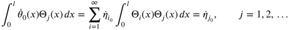
in view of the orthogonality of normal modes (Eq. [E10.3.8]). Using the initial values of ![]() and
and ![]() , Eqs. (10.74) and (10.75), the free vibration response of the shaft can be determined from Eqs. (10.69) and (10.64):
, Eqs. (10.74) and (10.75), the free vibration response of the shaft can be determined from Eqs. (10.69) and (10.64):

10.5 FORCED VIBRATION OF A UNIFORM SHAFT: MODAL ANALYSIS
The equation of motion of a uniform shaft subjected to distributed external torque, ![]() , is given by Eq. (10.23):
, is given by Eq. (10.23):
The solution of Eq. (10.77) using modal analysis is expressed as

where ![]() is the nth normalized normal mode and
is the nth normalized normal mode and ![]() is the nth generalized coordinate. The normal modes
is the nth generalized coordinate. The normal modes ![]() are determined by solving the eigenvalue problem
are determined by solving the eigenvalue problem
by applying the boundary conditions of the shaft. By substituting Eq. (10.78) into (10.77), we obtain
where

Using Eq. (10.79), Eq. (10.80) can be rewritten as
Multiplication of Eq. (10.82) by ![]() and integration from 0 to l result in
and integration from 0 to l result in

In view of the orthogonality relationships, Eq. (E10.3.8), Eq. (10.83) reduces to
where the normal modes are assumed to satisfy the normalization condition
and ![]() , called the generalized force in nth mode, is given by
, called the generalized force in nth mode, is given by

The complete solution of Eq. (10.84) can be expressed as
where the constants ![]() and
and ![]() can be determined from the initial conditions of the shaft. Thus, the forced vibration response of the shaft (i.e. the solution of Eq. [10.77]), is given by
can be determined from the initial conditions of the shaft. Thus, the forced vibration response of the shaft (i.e. the solution of Eq. [10.77]), is given by

The steady‐state response of the shaft, without considering the effect of initial conditions, can be obtained from Eq. (10.88), as

Note that if the shaft is unrestrained (free at both ends), the rigid‐body displacement, ![]() , is to be added to the solution given by Eq. (10.89). If
, is to be added to the solution given by Eq. (10.89). If ![]() denotes the torque applied to the shaft, the rigid‐body motion of the shaft,
denotes the torque applied to the shaft, the rigid‐body motion of the shaft, ![]() , can be determined from the relation
, can be determined from the relation

where ![]() denotes the mass moment of inertia of the shaft and
denotes the mass moment of inertia of the shaft and ![]() indicates the acceleration of rigid‐body motion.
indicates the acceleration of rigid‐body motion.
10.6 TORSIONAL VIBRATION OF NONCIRCULAR SHAFTS: SAINT‐VENANT'S THEORY
For a shaft or bar of noncircular cross‐section subjected to torsion, the cross‐sections do not simply rotate with respect to one another as in the case of a circular shaft, but they are deformed, too. The originally plane cross‐sections of the shaft do not remain plane but warp out of their own planes after twisting, as shown in Fig. 10.7. Thus, the points in the cross‐section undergo an axial displacement. A function ![]() , known as the warping function, is used to denote the axial displacement as
, known as the warping function, is used to denote the axial displacement as
where ![]() denotes the rate of twist along the shaft, assumed to be a constant. The other components of displacement in the shaft are given by
denotes the rate of twist along the shaft, assumed to be a constant. The other components of displacement in the shaft are given by
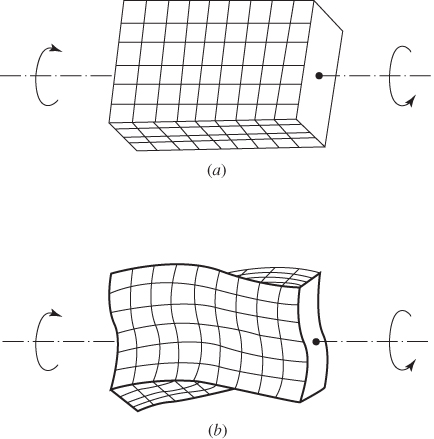
Figure 10.7 Shaft with rectangular cross‐section under torsion: (a) before deformation; (b) after deformation.
The strains are given by
The corresponding stresses can be determined as
The strain energy of the shaft is given by
Defining the torsional rigidity (C) of its noncircular section of the shaft as
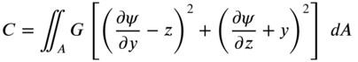
the strain energy of the shaft can be expressed as

Neglecting the inertia due to axial motion, the kinetic energy of the shaft can be written as in Eq. (10.11). The work done by the applied torque is given by Eq. (10.12). Hamilton's principle can be written as
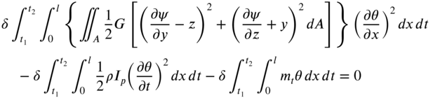
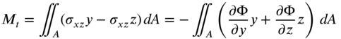
The first integral of Eq. (10.99) can be evaluated as

The first integral term on the right‐hand side of Eq. (10.100) can be expressed as (see Eq. [10.97])

The second integral term on the right‐hand side of Eq. (10.100) is set equal to zero independently:

Integrating Eq. (10.102) by parts, we obtain

where ![]() is the bounding curve of the cross‐section and
is the bounding curve of the cross‐section and ![]() is the cosine of the angle between the normal to the bounding curve and the
is the cosine of the angle between the normal to the bounding curve and the ![]() direction. Equation (10.103) yields the differential equation for the warping function
direction. Equation (10.103) yields the differential equation for the warping function ![]() as
as
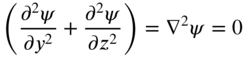
and the boundary condition on ![]() as
as
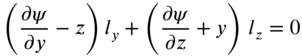
Physically, Eq. (10.105) represents that the shear stress normal to the boundary must be zero at every point on the boundary of the cross‐section of the shaft. When Eq. (10.101) is combined with the second and third integrals of Eq. (10.99), it leads to the equation of motion as
and the boundary conditions on ![]() as
as
10.7 TORSIONAL VIBRATION OF NONCIRCULAR SHAFTS, INCLUDING AXIAL INERTIA
Love included the inertia due to the axial motion caused by the warping of the cross‐section in deriving the equation of motion of a shaft in torsional vibration [4, 10]. In this case, the kinetic energy of the shaft is given by
where

Note that ![]() denotes the axial inertia term. The variation associated with
denotes the axial inertia term. The variation associated with ![]() in Hamilton's principle leads to
in Hamilton's principle leads to

Denoting

the integrals in Eq. (10.111) can be evaluated to obtain

The first, second, and third terms on the right‐hand side of Eq. (10.114) contribute to the equation of motion, Eq. (10.106), the boundary conditions on ![]() , Eq. (10.107), and to the differential equation for
, Eq. (10.107), and to the differential equation for ![]() , Eq. (10.104), respectively. The new equations are given by
, Eq. (10.104), respectively. The new equations are given by


where

10.8 TORSIONAL VIBRATION OF NONCIRCULAR SHAFTS: THE TIMOSHENKO–GERE THEORY
In this theory also, the displacement components of a point in the cross‐section are assumed to be [4, 11, 17]
where ![]() is not assumed to be a constant. The components of strains can be obtained as
is not assumed to be a constant. The components of strains can be obtained as


The components of stress are given by

that is,


Note that the effect of Poisson's ratio is neglected in Eqs. (10.130) and (10.131). The strain energy of the shaft can be determined as
where
The variation of the integral ![]() can be evaluated as
can be evaluated as
where

When the second term on the right‐hand side of Eq. (10.138) is integrated by parts, we obtain

The variation of the integral ![]() can be evaluated as indicated in Eqs. (10.100), (10.101) and (10.103). The expressions for the kinetic energy and the work done by the applied torque are given by Eqs. (10.108) and (10.12), respectively, and hence their variations can be evaluated as indicated earlier. The application of Hamilton's principle leads to the equation of motion for
can be evaluated as indicated in Eqs. (10.100), (10.101) and (10.103). The expressions for the kinetic energy and the work done by the applied torque are given by Eqs. (10.108) and (10.12), respectively, and hence their variations can be evaluated as indicated earlier. The application of Hamilton's principle leads to the equation of motion for ![]() :
:

and the boundary conditions

The differential equation for the warping function ![]() becomes
becomes

with the boundary condition on ![]() given by
given by

10.9 TORSIONAL RIGIDITY OF NONCIRCULAR SHAFTS
It is necessary to find the torsional rigidity C of the shaft in order to find the solution of the torsional vibration problem, Eq. (10.106). The torsional rigidity can be determined by solving the Laplace equation, Eq. (10.104):
subject to the boundary condition, Eq. (10.105):
which is equivalent to
Since the solution of Eq. (10.146), for the warping function ![]() , subject to the boundary condition of Eq. (10.147) or (10.148) is relatively more difficult, we use an alternative procedure which leads to a differential equation similar to Eq. (10.146), and a boundary condition that is much simpler in form than Eq. (10.147) or (10.148). For this we express the stresses
, subject to the boundary condition of Eq. (10.147) or (10.148) is relatively more difficult, we use an alternative procedure which leads to a differential equation similar to Eq. (10.146), and a boundary condition that is much simpler in form than Eq. (10.147) or (10.148). For this we express the stresses ![]() and
and ![]() in terms of a function
in terms of a function ![]() , known as the Prandtl stress function, as [3, 7]
, known as the Prandtl stress function, as [3, 7]
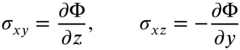
The stress field corresponding to Saint‐Venant's theory, Eq. (10.95), along with Eq. (10.149), satisfies the equilibrium equations:

By equating the corresponding expressions of ![]() and
and ![]() given by Eqs. (10.95) and (10.149), we obtain
given by Eqs. (10.95) and (10.149), we obtain
Differentiating Eq. (10.151) with respect to z and Eq. (10.152) with respect to y and subtracting the resulting equations one from the other leads to the Poisson equation:

where
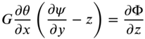
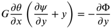
is assumed to be a constant. The condition to be satisfied by the stress function ![]() on the boundary can be derived by considering a small element of the rod at the boundary as shown in Fig. 10.8. The component of shear stress along the normal direction n can be expressed as
on the boundary can be derived by considering a small element of the rod at the boundary as shown in Fig. 10.8. The component of shear stress along the normal direction n can be expressed as
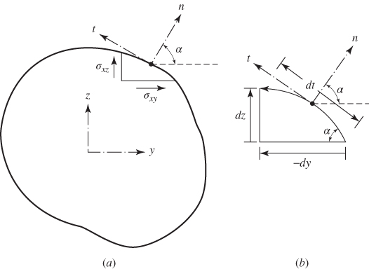
Figure 10.8 Boundary condition on the stresses.
since the boundary is stress‐free. In Eq. (10.155), the direction cosines are given by
where t denotes the tangential direction. Using Eq. (10.149), the boundary condition, Eq. (10.155), can be written as
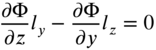
The rate of change of ![]() along the tangential direction at the boundary (t) can be expressed as
along the tangential direction at the boundary (t) can be expressed as

using Eqs. (10.156) and (10.157). Equation (10.158) indicates that the stress function ![]() is a constant on the boundary of the cross‐section of the rod. Since the magnitude of this constant does not affect the stress, which contains only derivatives of
is a constant on the boundary of the cross‐section of the rod. Since the magnitude of this constant does not affect the stress, which contains only derivatives of ![]() , we choose, for convenience,
, we choose, for convenience,
to be the boundary condition.
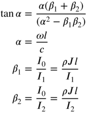
Next we derive a relation between the unknown angle ![]() (angle of twist per unit length) and the torque
(angle of twist per unit length) and the torque ![]() acting on the rod. For this, consider the cross‐section of the twisted rod, as shown in Fig. 10.9. The moment about the x axis of all the forces acting on a small elemental area dA located at the point
acting on the rod. For this, consider the cross‐section of the twisted rod, as shown in Fig. 10.9. The moment about the x axis of all the forces acting on a small elemental area dA located at the point ![]() is given by
is given by

Figure 10.9 Forces acting on the cross‐section of a rod under torsion.
The resulting moment can be found by integrating the expression in Eq. (10.160) over the entire area of cross‐section of the bar as
Each term under the integral sign in Eq. (10.161) can be integrated by parts to obtain (see Fig. 10.9):

since ![]() at the points
at the points ![]() and
and ![]() . Similarly,
. Similarly,

Thus, the torque on the cross‐section ![]() is given by
is given by
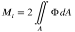
The function ![]() satisfies the linear differential (Poisson) equation given by Eq. (10.153) and depends linearly on
satisfies the linear differential (Poisson) equation given by Eq. (10.153) and depends linearly on ![]() , so that Eq. (10.164) produces an equation of the form
, so that Eq. (10.164) produces an equation of the form ![]() , where J is called the torsional constant (J is the polar moment of inertia of the cross‐section for a circular section) and C is called the torsional rigidity. Thus, Eq. (10.164) can be used to find the torsional rigidity (C).
, where J is called the torsional constant (J is the polar moment of inertia of the cross‐section for a circular section) and C is called the torsional rigidity. Thus, Eq. (10.164) can be used to find the torsional rigidity (C).
Note There are very few cross‐sectional shapes for which Eq. (10.164) can be evaluated in closed form to find an exact solution of the torsion problem. The following example indicates the procedure of finding an exact closed‐form solution for the torsion problem for an elliptic cross‐section.
10.10 PRANDTL'S MEMBRANE ANALOGY
Prandtl observed that the differential equation for the stress function, Eq. (10.153), is of the same form as the equation that describes the deflection of a membrane or soap film under transverse pressure (see Eq. [13.1] without the right‐hand‐side inertia term). This analogy between the torsion and membrane problems has been used in determining the torsional rigidity of rods with noncircular cross‐sections experimentally [3, 4]. An actual experiment with a soap bubble would consist of an airtight box with a hole cut on one side (Fig. 10.11). The shape of the hole is the same as the cross‐section of the rod in torsion. First, a soap film is created over the hole. Then air under pressure (p) is pumped into the box. This causes the soap film to deflect transversely as shown in Fig. 10.11. If P denotes the uniform tension in the soap film, the small transverse deflection of the soap film (w) is governed by the equation (see Eq. [13.1] without the right‐hand‐side inertia term)

Figure 10.11 Soap film for the membrane analogy.

or
in the hole region (cross‐section) and
on the boundary of the hole (cross‐section). Note that the differential equation and the boundary condition, Eqs. (10.166) and (10.167), are of precisely the same form as for the stress function ![]() , namely, Eqs. (10.153) and (10.159):
, namely, Eqs. (10.153) and (10.159):
in the interior, and
on the boundary. Thus, the soap bubble represents the surface of the stress function with
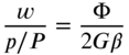
or
where ![]() denotes a proportionality constant:
denotes a proportionality constant:

The analogous quantities in the two cases are given in Table 10.2.
Table 10.2 Prandtl's membrane analogy.
| Soap bubble (membrane) problem | Torsion problem |
| G | |
| p | |
| 2 (volume under bubble) |
The membrane analogy provides more than an experimental technique for the solution of torsion problem. It also serves as the basis for obtaining approximate analytical solutions for rods with narrow cross‐sections and open thin‐walled cross‐sections. Table 10.3 gives the values of the maximum shear stress and the angle of twist per unit length for some commonly encountered cross‐sectional shapes of rods.
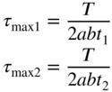
Table 10.3 Torsional properties of shafts with various cross‐sections.
| Cross‐section | Angle of twist per unit length, |
Maximum shear stress, |
|||||||||||||||||||||
1. Solid circular shaft
|
|||||||||||||||||||||||
2. Thick‐walled tube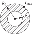 |
 |
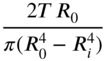 |
|||||||||||||||||||||
3. Thin‐walled tube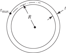 |
|||||||||||||||||||||||
4. Solid elliptic shaft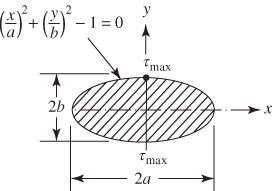 |
 |
||||||||||||||||||||||
5. Hollow elliptic tube |
 |
||||||||||||||||||||||
6. Solid square shaft |
|||||||||||||||||||||||
7. Solid rectangular shaft |
|
||||||||||||||||||||||
8. Hollow rectangular shaft
|
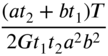 |
 |
|||||||||||||||||||||
9. Solid equilateral triangular shaft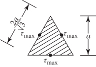 |
|||||||||||||||||||||||
10. Thin‐walled tube |
 |
10.11 RECENT CONTRIBUTIONS
The torsional vibration of tapered rods with rectangular cross‐section, pre‐twisted uniform rods, and pre‐twisted tapered rods is presented by Rao [4]. In addition, several refined theories of torsional vibration of rods are also presented in Ref. [4].
Torsional vibration of bars:
The torsional vibration of beams with a rectangular cross‐section is presented by Vet [8]. An overview of the vibration problems associated with turbomachinery is given by Vance [9]. The free vibration coupling of bending and torsion of a uniform spinning beam was studied by Filipich and Rosales [16]. The exact solution was presented and a numerical example was given to point out the influence of whole coupling.
Torsional vibration of thin‐walled beams:
The torsional vibration of beams of thin‐walled open section has been studied by Gere [11]. The behavior of torsion of bars with warping restraint is studied using Hamilton's principle by Lo and Goulard [12].
Vibration of a cracked rotor:
The coupling between the longitudinal, lateral, and torsional vibrations of a cracked rotor was studied by Darpe et al. [13]. In this work, the stiffness matrix of a Timoshenko beam element was modified to account for the effect of a crack and all six degrees of freedom per node were considered.
Torsional vibration control:
The torsional vibration control of a shaft through active constrained layer damping treatments has been studied by Shen et al. [14]. The equation of motion of the arrangement, consisting of piezoelectric and viscoelastic layers, is derived and its stability and controllability are discussed.
Torsional vibration of machinery drives:
The startup torque in an electrical induction motor can create problems when the motor is connected to mechanical loads, such as fans and pumps through shafts. The interrelationship between the electric motor and the mechanical system, which is effectively a multimass oscillatory system, has been examined by Ran et al. [15].
REFERENCES
- 1 W.F. Riley, L.D. Sturges, and D.H. Morris, Mechanics of Materials, 5th ed., Wiley, New York, 1999.
- 2 S. Timoshenko, D.H. Young, and W. Weaver, Jr., Vibration Problems in Engineering, 4th ed., Wiley, New York, 1974.
- 3 W.B. Bickford, Advanced Mechanics of Materials, Addison‐Wesley, Reading, MA, 1998.
- 4 J.S. Rao, Advanced Theory of Vibration, Wiley, New York, 1992.
- 5 S.K. Clark, Dynamics of Continuous Elements, Prentice‐Hall, Englewood Cliffs, NJ, 1972.
- 6 S.S. Rao, Mechanical Vibrations, 6th ed., Pearson Education, Inc., Hoboken, NJ, 2017.
- 7 J.H. Faupel and F.E. Fisher, Engineering Design, 2nd ed., Wiley‐Interscience, New York, 1981.
- 8 M. Vet, Torsional vibration of beams having rectangular cross‐sections, Journal of the Acoustical Society of America, Vol. 34, p. 1570, 1962.
- 9 J.M. Vance, Rotordynamics of Turbomachinery, Wiley, New York, 1988.
- 10 A.E.H. Love, A Treatise on the Mathematical Theory of Elasticity, 4th ed., Dover, New York, 1944.
- 11 J.M. Gere, Torsional vibrations of beams of thin walled open section, Journal of Applied Mechanics, Vol. 21, p. 381, 1954.
- 12 H. Lo and M. Goulard, Torsion with warping restraint from Hamilton's principle, Proceedings of the 2nd Midwestern Conference on Solid Mechanics, 1955, p. 68.
- 13 A.K. Darpe, K. Gupta, and A. Chawla, Coupled bending, longitudinal and torsional vibration of a cracked rotor, Journal of Sound and Vibration, Vol. 269, No. 1–2, pp. 33–60, 2004.
- 14 I.Y. Shen, W. Guo, and Y.C. Pao, Torsional vibration control of a shaft through active constrained layer damping treatments, Journal of Vibration and Acoustics, Vol. 119, No. 4, pp. 504–511, 1997.
- 15 L. Ran, R. Yacamini, and K.S. Smith, Torsional vibrations in electrical induction motor drives during start up, Journal of Vibration and Acoustics, Vol. 118, No. 2, pp. 242–251, 1996.
- 16 C.P. Filipich and M.B. Rosales, Free flexural–torsional vibrations of a uniform spinning beam, Journal of Sound and Vibration, Vol. 141, No. 3, pp. 375–387, 1990.
- 17 S.P. Timoshenko, Theory of bending, torsion and buckling of thin‐walled member of open cross‐section, Journal of the Franklin Institute, Vol. 239, pp. 201, 249, and 343, 1945.
PROBLEMS
- 10.1 A shaft with a uniform circular cross‐section of diameter d and length l carries a heavy disk of mass moment of inertia
 at the center. Find the first three natural frequencies and the corresponding modes of the shaft in torsional vibration. Assume that the shaft is fixed at both the ends.
 - 10.2 A shaft with a uniform circular cross‐section of diameter d and length l carries a heavy disk of mass moment of inertia
 at the center. If both ends of the shaft are fixed, determine the free vibration response of the system when the disk is given an initial angular displacement of
  and a zero initial angular velocity.
 - 10.3 A uniform shaft supported at
 and rotating at an angular velocity
  is suddenly stopped at the end
  . If the end
  is free and the cross‐section of the shaft is tubular with inner and outer radii
  and
and  , respectively, find the subsequent time variation of the angular displacement of the shaft.
 - 10.4 A uniform shaft of length l is fixed at
 and free at
  . Find the forced vibration response of the shaft if a torque
  is applied at the free end. Assume the initial conditions of the shaft to be zero.
 - 10.5 Find the first three natural frequencies of torsional vibration of a shaft of length 1 m and diameter 20 mm for the following end conditions:
- Both ends are fixed.
- One end is fixed and the other end is free.
- Both ends are free.
Material of the shaft: steel with
 and
and  .
. - 10.6 Solve Problem 10.5 by assuming the material of the shaft to be aluminum with
 and
and  .
. - 10.7 Consider two shafts each of length l with thin‐walled tubular sections, one in the form of a circle and the other in the form of a square, as shown in Fig. 10.13.

Figure 10.13 Circular and square tubular sections of a shaft.
Assuming the same wall thickness of the tubes and the same total area of the region occupied by the material (material area), compare the fundamental natural frequencies of the torsional vibration of the shafts. Assume the shaft to be fixed at both the ends.
- 10.8 Solve Problem 10.7 by assuming the tube wall thickness and the interior cavity areas of the tubes to be the same.
- 10.9 Determine the velocity of propagation of torsional waves in the drive shaft of an automobile for the following data:
- Cross‐section: circular with diameter 100 mm; material: steel with
 and
and  .
. - Cross‐section: hollow with inner diameter 80 mm and outer diameter 120 mm; material: aluminum with
 and
and  .
.
- Cross‐section: circular with diameter 100 mm; material: steel with
- 10.10 Find the first three natural frequencies of torsional vibration of a shaft fixed at
 and a disk of mass moment of inertia
  attached at
  . Shaft: uniform circular cross‐section of diameter 20 mm and length 1 m; material of shaft: steel with
  and
and  .
. - 10.11 Find the fundamental natural frequency of torsional vibration of the shaft described in Problem 10.10 using a single‐degree‐of‐freedom model.
- 10.12 Find the free torsional vibration response of a uniform shaft of length l subjected to an initial angular displacement
 and an initial angular velocity
  using modal analysis. Assume the shaft to be fixed at
  and free at
  .
. - 10.13 Find the free torsional vibration response of a uniform shaft of length l subjected to an initial angular displacement
 and an initial angular velocity
  using modal analysis. Assume the shaft to be fixed at
  and free at
  .
. - 10.14 Derive the frequency equation for the torsional vibration of a uniform shaft with a torsional spring of stiffness
 attached to each end.
 - 10.15 Find the steady‐state response of a shaft fixed at both ends when subjected to a torque
 at
at  using modal analysis.
 - 10.16 A shaft with a uniform circular cross‐section of diameter d and length l is fixed at
 and carries a heavy disk of mass moment of inertia
  at the other end
  . Derive the frequency equation for the torsional vibration of the shaft.
 - 10.17 Consider two shafts each of length l with thin‐walled tubular sections, one in the form of a circle and the other in the form of a square, as shown in Fig. 10.13. Compare the angles of twist per unit length of the two shafts for unit torque.
- 10.18 Consider two shafts each of length l with thin‐walled tubular sections, one in the form of a circle and the other in the form of a square, as shown in Fig. 10.13. What is the difference in the fundamental natural frequencies of vibration of the two shafts?
- 10.19 A uniform circular shaft of polar area moment of inertia
 and polar mass moment of inertia
  and length l is fixed at one end and free at the other end. Find the free vibration response of the shaft.