8
Transverse Vibration of Strings
8.1 INTRODUCTION
It is well known that most important musical instruments, including the violin and the guitar, involve strings whose natural frequencies and mode shapes play a significant role in their performance. The characteristics of many engineering systems, such as guy wires, electric transmission lines, ropes and belts used in machinery, and thread manufacture, can be derived from a study of the dynamics of taut strings. The free and forced transverse vibration of strings is considered in this chapter. As will be seen in subsequent chapters, the equation governing the transverse vibration of strings will have the same form as the equations of motion of longitudinal vibration of bars and torsional vibration of shafts.
8.2 EQUATION OF MOTION
8.2.1 Equilibrium Approach
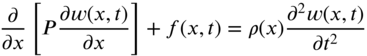
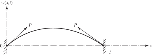
Figure 8.1 shows a tightly stretched elastic string or cable of length l subjected to a distributed transverse force ![]() per unit length. The string is assumed to be supported at the ends on elastic springs of stiffness
per unit length. The string is assumed to be supported at the ends on elastic springs of stiffness ![]() and
and ![]() . By assuming the transverse displacement of the string
. By assuming the transverse displacement of the string ![]() to be small, Newton's second law of motion can be applied for the motion of an element of the string in the z direction as
to be small, Newton's second law of motion can be applied for the motion of an element of the string in the z direction as

Figure 8.1 (a) Vibrating string; (b) differential element.
If ![]() is the tension,
is the tension, ![]() is the mass per unit length, and
is the mass per unit length, and ![]() is the angle made by the deflected string with the x axis, Eq. (8.1) can be rewritten, for an element of length
is the angle made by the deflected string with the x axis, Eq. (8.1) can be rewritten, for an element of length ![]() , as
, as

Noting that

Eq. (8.2) can be expressed as
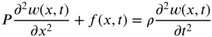
If the string is uniform and the tension is constant, Eq. (8.6) takes the form
For free vibration, ![]() and Eq. (8.7) reduces to
and Eq. (8.7) reduces to

which can be rewritten as
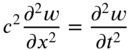
where
Equation (8.9) is called the one‐dimensional wave equation.
8.2.2 Variational Approach
Strain Energy There are three sources of strain energy for the taut string shown in Fig. 8.1. The first is due to the deformation of the string over ![]() , where the tension
, where the tension ![]() tries to restore the deflected string to the equilibrium position; the second is due to the deformation of the spring at
tries to restore the deflected string to the equilibrium position; the second is due to the deformation of the spring at ![]() ; and the third is due to the deformation of the spring at
; and the third is due to the deformation of the spring at ![]() . The length of a differential element dx in the deformed position, ds, can be expressed as
. The length of a differential element dx in the deformed position, ds, can be expressed as

by assuming the slope of the deflected string, ![]() , to be small. The strain energy due to the deformations of the springs at
, to be small. The strain energy due to the deformations of the springs at ![]() and
and ![]() is given by
is given by ![]() and
and ![]() , and the strain energy associated with the deformation of the string is given by the work done by the tensile force
, and the strain energy associated with the deformation of the string is given by the work done by the tensile force ![]() while moving through the distance
while moving through the distance ![]() :
:

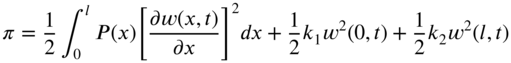
Thus, the total strain energy, ![]() , is given by
, is given by
Kinetic Energy The kinetic energy of the string is given by
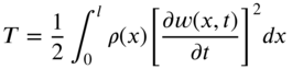
where ![]() is the mass of the string per unit length.
is the mass of the string per unit length.
Work Done by External Forces The work done by the nonconservative distributed load acting on the string, ![]() , can be expressed as
, can be expressed as

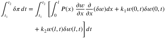
Hamilton's principle gives

or

The variations of the individual terms appearing in Eq. (8.17) can be carried out as follows:

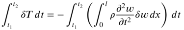
using the interchangeability of the variation and differentiation processes. Equation (8.18) can be evaluated by using integration by parts with respect to time:

Using the fact that ![]() at
at ![]() and
and ![]() and assuming
and assuming ![]() to be constant, Eq. (8.19) yields
to be constant, Eq. (8.19) yields
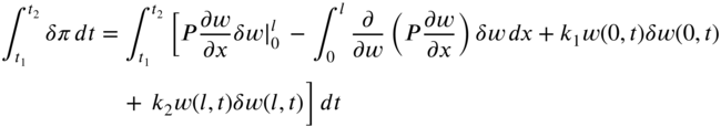
The second term of Eq. (8.16) can be written as
By using integration by parts with respect to x, Eq. (8.21) can be expressed as
The third term of Eq. (8.16) can be written as

By inserting Eqs. (8.20), (8.22), and (8.23) into Eq. (8.16) and collecting the terms, we obtain

Since the variation ![]() over the interval
over the interval ![]() is arbitrary, Eq. (8.24) can be satisfied only when the individual terms of Eq. (8.24) are equal to zero:
is arbitrary, Eq. (8.24) can be satisfied only when the individual terms of Eq. (8.24) are equal to zero:

Equation (8.25) denotes the equation of motion while Eqs. (8.26) and (8.27) represent the boundary conditions. Equation (8.26) can be satisfied when ![]() or when
or when ![]() . Since the displacement
. Since the displacement ![]() cannot be zero for all time at
cannot be zero for all time at ![]() , Eq. (8.26) can only be satisfied by setting
, Eq. (8.26) can only be satisfied by setting
Similarly, Eq. (8.27) leads to the condition
Thus, the differential equation of motion of the string is given by Eq. (8.25) and the corresponding boundary conditions by Eqs. (8.28) and (8.29).
8.3 INITIAL AND BOUNDARY CONDITIONS
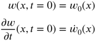
The equation of motion, Eq. (8.6), or its special forms Eqs. (8.7) and (8.8) or (8.9), is a partial differential equation of order 2 in x as well as t. Thus, two boundary conditions and two initial conditions are required to find the solution, ![]() . If the string is given an initial deflection
. If the string is given an initial deflection ![]() and an initial velocity
and an initial velocity ![]() , the initial conditions can be stated as
, the initial conditions can be stated as
If the string is fixed at ![]() , the displacement is zero and hence the boundary conditions will be
, the displacement is zero and hence the boundary conditions will be
If the string is connected to a pin that is free to move in a transverse direction, the end will not be able to support any transverse force, and hence the boundary condition will be
If the axial force is constant and the end ![]() is free, Eq. (8.32) becomes
is free, Eq. (8.32) becomes
If the end ![]() of the string is connected to an elastic spring of stiffness k, the boundary condition will be
of the string is connected to an elastic spring of stiffness k, the boundary condition will be

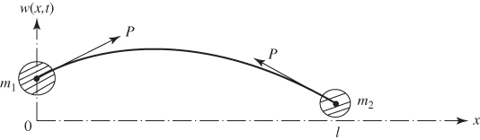
Some of the possible boundary conditions of a string are summarized in Table 8.1.
Table 8.1 Boundary conditions of a string.
| Support conditions of the string | Boundary conditions to be satisfied |
| 1. Both ends fixed | |
|
 |
| 2. Both ends free | |
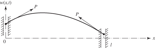 |
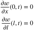 |
| 3. Both ends attached with masses | |
|
 |
| 4. Both ends attached with springs | |

|
 |
| 5. Both ends attached with dampers | |
|
 |
8.4 FREE VIBRATION OF AN INFINITE STRING
Consider a string of infinite length. The free vibration equation of the string, Eq. (8.9), is solved using three different approaches in this section.
8.4.1 Traveling‐Wave Solution
The solution of the wave equation (8.9) can be expressed as
where ![]() and
and ![]() are arbitrary functions of
are arbitrary functions of ![]() and
and ![]() , respectively. The solution given by Eq. (8.35) is known as D'Alembert's solution. The validity of Eq. (8.35) can be established by differentiating Eq. (8.35) as
, respectively. The solution given by Eq. (8.35) is known as D'Alembert's solution. The validity of Eq. (8.35) can be established by differentiating Eq. (8.35) as
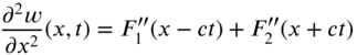
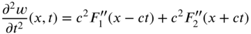
where a prime indicates a derivative with respect to the respective argument. By substituting Eqs. (8.36) and (8.37) into Eq. (8.9), we find that Eq. (8.9) is satisfied. The functions ![]() and
and ![]() denote waves that propagate in the positive and negative directions of the x axis, respectively, with a velocity c. The functions
denote waves that propagate in the positive and negative directions of the x axis, respectively, with a velocity c. The functions ![]() and
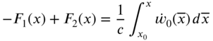
and ![]() can be determined from the known initial conditions of the string. Using the initial conditions of Eq. (8.30), Eq. (8.35) yields
can be determined from the known initial conditions of the string. Using the initial conditions of Eq. (8.30), Eq. (8.35) yields
where a prime in Eq. (8.39) denotes a derivative with respect to the respective argument at ![]() (i.e. with respect to x). By integrating Eq. (8.39) with respect to x, we obtain
(i.e. with respect to x). By integrating Eq. (8.39) with respect to x, we obtain
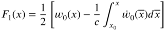
where ![]() is a constant. Equations (8.38) and (8.40) can be solved to find
is a constant. Equations (8.38) and (8.40) can be solved to find ![]() and
and ![]() as
as

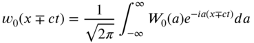
By replacing x by ![]() and
and ![]() , respectively, in Eqs. (8.41) and (8.42), we can express the wave solution of the string,
, respectively, in Eqs. (8.41) and (8.42), we can express the wave solution of the string, ![]() , as
, as
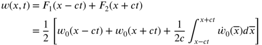
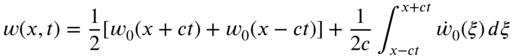
The solution given by Eq. (8.43) can be rewritten as
where ![]() represents a wave propagating due to a known initial displacement
represents a wave propagating due to a known initial displacement ![]() with zero initial velocity, and
with zero initial velocity, and ![]() indicates a wave moving due to the initial velocity
indicates a wave moving due to the initial velocity ![]() with zero initial displacement. A typical wave traveling due to initial displacement (introduced by pulling the string slightly in the transverse direction with zero velocity) is shown in Fig. 8.2.
with zero initial displacement. A typical wave traveling due to initial displacement (introduced by pulling the string slightly in the transverse direction with zero velocity) is shown in Fig. 8.2.

Figure 8.2 Propagation of a wave caused by an initial displacement.
8.4.2 Fourier Transform‐Based Solution
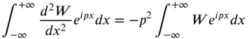
To find the free vibration response of an infinite string ![]() under the initial conditions of Eq. (8.30), we take the Fourier transform of Eq. (8.9). For this, we multiply Eq. (8.9) by
under the initial conditions of Eq. (8.30), we take the Fourier transform of Eq. (8.9). For this, we multiply Eq. (8.9) by ![]() and integrate from
and integrate from ![]() to
to ![]() :
:
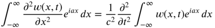
Integration of the left‐hand side of Eq. (8.45) by parts results in

Assuming that both ![]() and
and ![]() tend to zero as
tend to zero as ![]() , the first term on the right‐hand side of Eq. (8.46) vanishes. Using Eq. (7.16), the Fourier transform of
, the first term on the right‐hand side of Eq. (8.46) vanishes. Using Eq. (7.16), the Fourier transform of ![]() is defined as
is defined as

and Eq. (8.45) can be rewritten in the form
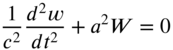
Note that the use of the Fourier transform reduced the partial differential equation (8.9) into the ordinary differentiation equation (8.48). The solution of Eq. (8.48) can be expressed as
where the constants ![]() and
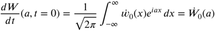
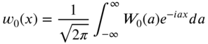
and ![]() can be evaluated using the initial conditions, Eqs. (8.30). By taking the Fourier transforms of the initial displacement
can be evaluated using the initial conditions, Eqs. (8.30). By taking the Fourier transforms of the initial displacement ![]() and initial velocity
and initial velocity ![]() , we obtain
, we obtain

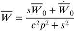
The use of Eqs. (8.50) and (8.51) in Eq. (8.49) leads to
whose solution gives

Thus, Eq. (8.49) can be expressed as
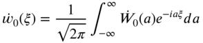
By using the inverse Fourier transform of Eq. (8.47), we obtain
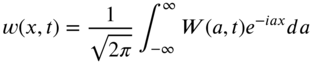
which, in view of Eq. (8.56), becomes
Note that the inverse Fourier transforms of ![]() and
and ![]() , Eqs. (8.50) and (8.51), can be obtained as
, Eqs. (8.50) and (8.51), can be obtained as
so that
By integrating Eq. (8.60) with respect to ![]() from
from ![]() to
to ![]() , we obtain
, we obtain

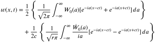
When Eqs. (8.61) and (8.62) are substituted into Eq. (8.58), we obtain

which can be seen to be identical to Eq. (8.43).
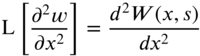
8.4.3 Laplace Transform‐Based Solution
The Laplace transforms of the terms in the governing equation (8.9) lead to

where
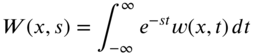
Using Eqs. (8.64) and (8.65) along with the initial conditions of Eq. (8.30), Eq. (8.9) can be expressed as

Now, we take the Fourier transform of Eq. (8.67). For this, we multiply Eq. (8.67) by ![]() and integrate with respect to x from
and integrate with respect to x from ![]() to
to ![]() , to obtain
, to obtain

The integral on the left‐hand side of Eq. (8.68) can be evaluated by parts:

Assuming that the deflection, ![]() , and the slope,
, and the slope, ![]() , tend to be zero as
, tend to be zero as ![]() , Eq. (8.69) reduces to
, Eq. (8.69) reduces to
and hence Eq. (8.68) can be rewritten as

or
or
where


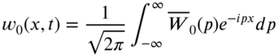
Now we first take the inverse Fourier transform of ![]() to obtain
to obtain

and next we take the inverse Laplace transform of ![]() to obtain
to obtain
Noting that
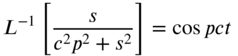
and

Eqs. (8.76) and (8.75) yield

where

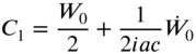
From Eqs. (8.80) and (8.81), we can write

In addition, the following identities are valid:
Thus, Eq. (8.79) can be rewritten as
which can be seen to be the same as the solution given by Eqs. (8.43) and (8.63). Note that Fourier transforms were used in addition to Laplace transforms in the current approach.
8.5 FREE VIBRATION OF A STRING OF FINITE LENGTH
The solution of the free vibration equation, Eq. (8.9), can be found using the method of separation of variables. In this method, the solution is written as
where ![]() is a function of x only and
is a function of x only and ![]() is a function of t only. By substituting Eq. (8.87) into Eq. (8.9), we obtain
is a function of t only. By substituting Eq. (8.87) into Eq. (8.9), we obtain
Noting that the left‐hand side of Eq. (8.88) depends only on x while the right‐hand side depends only on t, their common value must be a constant, a, and hence

Equation (8.89) can be written as two separate equations:


The constant a is usually negative1 and hence, by setting ![]() , Eqs. (8.90) and (8.91) can be rewritten as
, Eqs. (8.90) and (8.91) can be rewritten as

The solution of Eqs. (8.92) and (8.93) can be expressed as
where ![]() is the frequency of vibration, the constants A and B can be evaluated from the boundary conditions, and the constants C and D can be determined from the initial conditions of the string.
is the frequency of vibration, the constants A and B can be evaluated from the boundary conditions, and the constants C and D can be determined from the initial conditions of the string.
8.5.1 Free Vibration of a String with Both Ends Fixed
If the string is fixed at both ends, the boundary conditions are given by
Equations (8.96) and (8.94) yield
The condition of Eq. (8.97) requires that
in Eq. (8.94). Using Eqs. (8.98) and (8.99) in Eq. (8.94), we obtain
For a nontrivial solution, B cannot be zero and hence
Equation (8.101) is called the frequency or characteristic equation, and the values of ω that satisfy Eq. (8.101) are called the eigenvalues (or characteristic values or natural frequencies) of the string. The nth root of Eq. (8.101) is given by

and hence the nth natural frequency of vibration of the string is given by
The transverse displacement of the string, corresponding to ![]() , known as the nth mode of vibration or nth harmonic or nth normal mode of the string is given by
, known as the nth mode of vibration or nth harmonic or nth normal mode of the string is given by
In the nth mode, each point of the string vibrates with an amplitude proportional to the value of ![]() at that point with a circular frequency
at that point with a circular frequency ![]() . The first four modes of vibration are shown in Fig. 8.3. The mode corresponding to
. The first four modes of vibration are shown in Fig. 8.3. The mode corresponding to ![]() is called the fundamental mode,
is called the fundamental mode, ![]() is called the fundamental frequency, and
is called the fundamental frequency, and

Figure 8.3 Mode shapes of a string.
is called the fundamental period. The points at which ![]() for
for ![]() are called nodes. It can be seen that the fundamental mode has two nodes (at
are called nodes. It can be seen that the fundamental mode has two nodes (at ![]() and
and ![]() ), the second mode has three nodes (at
), the second mode has three nodes (at ![]() , and
, and ![]() ), and so on.
), and so on.
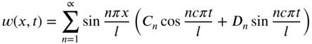
The free vibration of the string, which satisfies the boundary conditions of Eqs. (8.97) and (8.98), can be found by superposing all the natural modes ![]() as
as
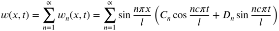
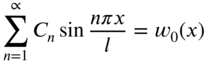
This equation represents the general solution of Eq. (8.9) and includes all possible vibrations of the string. The particular vibration that occurs is uniquely determined by the initial conditions specified. The initial conditions provide unique values of the constants ![]() and
and ![]() in Eq. (8.106). For the initial conditions stated in Eq. (8.30), Eq. (8.106) yields
in Eq. (8.106). For the initial conditions stated in Eq. (8.30), Eq. (8.106) yields
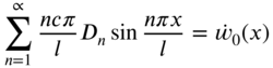
Noting that Eqs. (8.107) and (8.108) denote Fourier sine series expansions of ![]() and
and ![]() in the interval
in the interval ![]() , the values of
, the values of ![]() and
and ![]() can be determined by multiplying Eqs. (8.107) and (8.108) by
can be determined by multiplying Eqs. (8.107) and (8.108) by ![]() and integrating with respect to x from 0 to l. This gives the constants
and integrating with respect to x from 0 to l. This gives the constants ![]() and
and ![]() as
as


Note that the solution given by Eq. (8.106) represents the method of mode superposition since the response is expressed as a superposition of the normal modes. As indicated earlier, the procedure is applicable in finding not only the free vibration response but also the forced vibration response of any continuous system.
Notes
- If
 and
and  are both large,
  and
and  and the frequency equation, Eq. (E8.3.10), reduces to
Equation (E8.3.17) corresponds to the frequency equation of a wire with both ends fixed.
- If
 and
and  are both small,
  and
and  , and Eq. (E8.3.14) gives the frequencies as
(E8.3.18)
, and Eq. (E8.3.14) gives the frequencies as
(E8.3.18)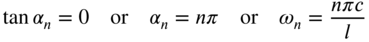
and Eq. (E8.3.16) yields the modal functions as
(E8.3.19)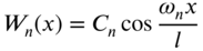
It can be observed that this solution corresponds to that of a wire with both ends free.
- If
 is large and
  is small,
  and
and  , and Eq. (E8.3.10) yields

or
(E8.3.20)
and Eq. (E8.3.16) gives the modal functions as
(E8.3.21)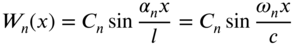
This solution corresponds to that of a wire which is fixed at
 and free at
  .
.

8.6 FORCED VIBRATION
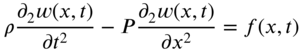
The equation of motion governing the forced vibration of a uniform string subjected to a distributed load ![]() per unit length is given by
per unit length is given by
Let the string be fixed at both ends so that the boundary conditions become
The solution of the homogeneous equation (with ![]() in Eq. [8.111]), which represents free vibration, can be expressed as (see Eq. [8.106])
in Eq. [8.111]), which represents free vibration, can be expressed as (see Eq. [8.106])
The solution of the nonhomogeneous equation (with ![]() in Eq. [8.111]), which also satisfies the boundary conditions of Eqs. (8.112) and (8.113), can be assumed to be of the form
in Eq. [8.111]), which also satisfies the boundary conditions of Eqs. (8.112) and (8.113), can be assumed to be of the form

where ![]() denotes the generalized coordinates. By substituting Eq. (8.115) into Eq. (8.111), we obtain
denotes the generalized coordinates. By substituting Eq. (8.115) into Eq. (8.111), we obtain

Multiplication of Eq. (8.116) by ![]() and integration from 0 to l, along with the use of the orthogonality of the functions
and integration from 0 to l, along with the use of the orthogonality of the functions ![]() , leads to
, leads to
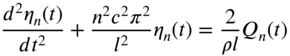
where
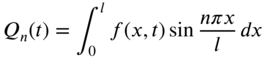
The solution of Eq. (8.117), including the homogeneous solution and the particular integral, can be expressed as

Thus, in view of Eq. (8.115), the forced vibration response of the string is given by
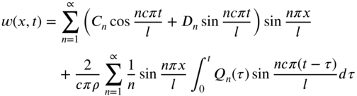
where the constants ![]() and
and ![]() are determined from the initial conditions of the string.
are determined from the initial conditions of the string.
8.7 RECENT CONTRIBUTIONS
The D'Alembert's solution of Eq. (8.8), as given by Eq. (8.35), is obtained by assuming that the increase in tension due to stretching is negligible. If this assumption is not made, Eq. (8.9) becomes

where

with ![]() denoting the density of the string. Here
denoting the density of the string. Here ![]() denotes the speed of compressional longitudinal wave through the string. An approximate solution of Eq. (8.121) was presented by Bolwell [4]. The dynamics of cables, chains, taut inclined cables, and hanging cables was considered by Triantafyllou [5,6]. In particular, the problem of linear transverse vibration of an elastic string hanging freely under its own weight presents a paradox, in that a solution can be obtained only when the lower end is free. An explanation of the paradox was given by Triantafyllou [6], who also showed that the paradox can be removed by including bending stiffness using singular perturbations.
denotes the speed of compressional longitudinal wave through the string. An approximate solution of Eq. (8.121) was presented by Bolwell [4]. The dynamics of cables, chains, taut inclined cables, and hanging cables was considered by Triantafyllou [5,6]. In particular, the problem of linear transverse vibration of an elastic string hanging freely under its own weight presents a paradox, in that a solution can be obtained only when the lower end is free. An explanation of the paradox was given by Triantafyllou [6], who also showed that the paradox can be removed by including bending stiffness using singular perturbations.
A mathematical model of the excitation of a vibrating system by a plucking action was studied by Griffel [7]. The mechanism is of the type used in musical instruments [8]. The effectiveness of the mechanism is computed over a range of the relevant parameters. In Ref. [9], Simpson derived the equations of in‐plane motion of an elastic catenary translating uniformly between its end supports in a Eulerian frame of reference. The approximate analytical solution of these equations is given for a shallow catenary in which the tension is dominated by the cable section modulus. Although the mathematical description of a vibrating string is given by the wave equation, a quantum model of information theory was used by Barrett to obtain a one‐degree‐of‐freedom mechanical system governed by a second‐order differential equation [10].
The vibration of a sectionally uniform string from an initial state was considered by Beddoe [11]. The problem was formulated in terms of reflections and transmissions of progressive waves and solved using the Laplace transform method without incorporating the orthogonality relationships. The exact equations of motion of a string were formulated by Narasimha [12], and a systematic procedure was described for obtaining approximations to the equations to any order, making only the assumption that the strain in the material of the string is small. It was shown that the lowest‐order equations in the scheme, which were nonlinear, were used to describe the response of the string near resonance.
Electrodischarge machining (EDM) is a noncontact process of electrically removing (cutting) material from conductive workpieces. In this process, a high potential difference is generated between a wire and a workpiece by charging them positively and negatively, respectively. The potential difference causes sparks between the wires and the workpiece. By moving the wire forward and sideways, the contour desired can be cut on the workpiece. In Ref. [13], Shahruz developed a mathematical model for the transverse vibration of the moving wire used in the EDM process in the form of a nonlinear partial differential equation. The equation was solved, and it was shown that the transverse vibration of the wire is stable and decays to zero for wire axial speeds below a critical value.
A comprehensive view of cable structures was presented by Irvine [14]. The natural frequencies and mode shapes of cables with attached masses have been determined by Sergev and Iwan [15]. The linear theory of free vibrations of a suspended cable has been outlined by Irvine and Caughey [16]. Yu presented explicit vibration solutions of a cable under complicated loads [17]. A theoretical and experimental analysis of free and forced vibration of sagged cable/mass suspension has been presented by Cheng and Perkins [18]. The linear dynamics of a translating string on an elastic foundation was considered by Perkins [19].
NOTE
- To show that a is usually a negative quantity, multiply Eq. (8.90) by
 and integrate with respect to x from 0 to l to obtain
Equation (a) indicates that the sign of a will be same as the sign of the integral on the left‐hand side. The left‐hand side of Eq. (a) can be integrated by parts to obtain
The first term on the right‐hand side of Eq. (b) can be seen to be zero or negative for a string with any combination of fixed end
 , free end
  , or elastically supported end
  , where k is the spring constant of the elastic support. Thus, the integral on the left‐hand side of Eq. (a), and hence the sign of a is negative.
REFERENCES
- 1 W. Nowacki, Dynamics of Elastic Systems, translated by H. Zorski, Wiley, New York, 1963.
- 2 N.W. McLachlan, Theory of Vibrations, Dover, New York, 1951.
- 3 S. Timoshenko, D.H. Young, and W. Weaver, Jr., Vibration Problems in Engineering, 4th ed., Wiley, New York, 1974.
- 4 J.E. Bolwell, The flexible string's neglected term, Journal of Sound and Vibration, Vol. 206, No. 4, pp. 618–623, 1997.
- 5 M.S. Triantafyllou, Dynamics of cables and chains, Shock and Vibration Digest, Vol. 19, pp. 3–5, 1987.
- 6 M.S. Triantafyllou and G.S. Triantafyllou, The paradox of the hanging string: an explanation using singular perturbations, Journal of Sound and Vibration, Vol. 148, No. 2, pp. 343–351, 1991.
- 7 D.H. Griffel, The dynamics of plucking, Journal of Sound and Vibration, Vol. 175, No. 3, pp. 289–297, 1994.
- 8 N.H. Fletcher and T.D. Rossing, The Physics of Musical Instruments, Springer‐Verlag, New York, 1991.
- 9 A. Simpson, On the oscillatory motions of translating elastic cables, Journal of Sound and Vibration, Vol. 20, No. 2, pp. 177–189, 1972.
- 10 T.W. Barrett, On vibrating strings and information theory, Journal of Sound and Vibration, Vol. 20, No. 3, pp. 407–412, 1972.
- 11 B. Beddoe, Vibration of a sectionally uniform string from an initial state, Journal of Sound and Vibration, Vol. 4, No. 2, pp. 215–223, 1966.
- 12 R. Narasimha, Non‐linear vibration of an elastic string, Journal of Sound and Vibration, Vol. 8, No. 1, pp. 134–146, 1968.
- 13 S.M. Shahruz, Vibration of wires used in electro‐discharge machining, Journal of Sound and Vibration, Vol. 266, No. 5, pp. 1109–1116, 2003.
- 14 H.M. Irvine, Cable Structures, MIT Press, Cambridge, MA, 1981.
- 15 S.S. Sergev and W.D. Iwan, The natural frequencies and mode shapes of cables with attached masses, Journal of Energy Resources Technology, Vol. 103, pp. 237–242, 1981.
- 16 H.M. Irvine and T.K. Caughey, The linear theory of free vibrations of a suspended cable, Proceedings of the Royal Society, London, Vol. A‐341, pp. 299–315, 1974.
- 17 P. Yu, Explicit vibration solutions of a cable under complicated loads, Journal of Applied Mechanics, Vol. 64, No. 4, pp. 957–964, 1997.
- 18 S.‐P. Cheng and N.C. Perkins, Theoretical and experimental analysis of the forced response of sagged cable/mass suspension, Journal of Applied Mechanics, Vol. 61, No. 4, pp. 944–948, 1994.
- 19 N.C. Perkins, Linear dynamics of a translating string on an elastic foundation, Journal of Vibration and Acoustics, Vol. 112, No. 1, pp. 2–7, 1990.
PROBLEMS
- 8.1 Find the free vibration response of a fixed–fixed string of length l which is given an initial displacement
and initial velocity
 .
. - 8.2 A steel wire of diameter
 . and length 3 ft is fixed at both ends and is subjected to a tension of 200 lb. Find the first four natural frequencies and the corresponding mode shapes of the wire.
 - 8.3 Determine the stress that needs to be applied to the wire of Problem 8.2 to reduce its fundamental natural frequency of vibration by 50% of the value found in Problem 8.2.
- 8.4 A string of length l is fixed at
 and subjected to a transverse force
  at
at  . Find the resulting vibration of the string.
 - 8.5 Find the forced vibration response of a fixed–fixed string of length l that is subjected to the distributed transverse force
 .
. - 8.6 A uniform string of length l is fixed at both ends and is subjected to the following initial conditions:

Find the response of the string.
- 8.7 Derive the boundary conditions corresponding to support conditions 3, 4, and 5 of Table 8.1 from equilibrium considerations.
- 8.8 The transverse vibration of a string of length
 is governed by the equation

The boundary and initial conditions of the string are given by

Find the displacement of the string,
 .
. - 8.9 A semi‐infinite string has one end at
 and the other end at
  . It is initially at rest on the x axis and the end
  is made to oscillate with a transverse displacement of
  . Find the transverse displacement of the string,
  .
. - 8.10 Find the natural frequencies of transverse vibration of a taut string of length l resting on linear springs of stiffnesses
 and
and  at the ends
  and
and  , respectively. Assume the following data:
  , and
, and  .
. - 8.11 Find the traveling‐wave solution of an infinite string presented in Section 8.4.1 by solving the equation of motion

with the initial conditions
 and
and  by using Laplace transforms with respect to t and Fourier transforms with respect to x.