
CHAPTER 11
A Review of A/V Basics
CONTENTS
11.0 Introduction to A/V Basics
11.1 A Digital View of an Analog World
11.2 Progressive and Interlace Images
11.4 Video Resolutions and Aspect Ratios
11.4.1 Aspect Ratio Conversions
11.5 Video Signal Representations
11.5.1 The RGB and R ’G’B’ Signals
11.5.2 The Component Color Difference Signals
11.5.3 The Y ’PrPb Component Analog Signal
11.5.4 The Y ’CrCb Component Digital Signal
11.5.5 The Analog Composite Video Signal
11.5.7 Analog and Digital Broadcast Standards
11.5.8 Professional Signal Formats—Some Conclusions
11.6 SDI Review—The Ubiquitous A/V Digital Link
11.6.2 The Proteus Clip Server Example
11.7 Video Signal Processing and Its Applications
11.7.1 Interlace to Progressive Conversion—Deinterlacing
11.7.3 Compressed Domain Processing
11.8 A/V Bit Rate Reduction Techniques
11.8.1 Audio Bit Rate Reduction Techniques
11.8.2 Video Compression Overview
11.8.3 Summary of Lossy Video Compression Techniques
11.10 It’s a Wrap—Some Final Words
11.0 INTRODUCTION TO A/V BASICS
Coverage in the other chapters has been purposely skewed toward the convergence of A/V + IT and the interrelationships of these for creating workflows. This chapter reviews traditional video and audio technology as standalone subjects without regard to IT. If you are savvy in A/V ways and means, then skip this chapter. However, if chroma, luma, gamma, and sync are foreign terms, then dig in for a working knowledge. Chapter 7 presented an overview of the three planes: user/data, control, and management. This chapter focuses on the A/V user/data plane and the nature of video signals in particular. Unfortunately, by necessity, explanations use acronyms that you may not be familiar with, so check the Glossary as needed.
The plan of attack in this chapter is as follows: an overview of video fundamentals including signal formats, resolutions, A/V interfaces, signal processing, compression methods, and time code basics.
11.1 A DIGITAL VIEW OF AN ANALOG WORLD
Despite the trend for all things digital, we live in an analog world. In 1876, Bell invented his “electrical speech machine,” as he called it—the telephone—a great example of analog design. However, analog signals are susceptible to noise, are not easily processed, are not networkable, suffer loss during transmission, and are difficult to store. Digital representations of analog signals generally overcome these negatives. Sure, digital has its trade-offs, but in the balance it wins out for many applications. Figure 11.1 shows the classic transform from the analog domain to the digital. Transformation is performed by an A-to-D converter that outputs a digital value every sample period at rate Fs. Better yet, some digital video and audio signals are never in analog form but are natively created with software or hardware. Often, but not always, the digital signal is converted back to analog using a D-to-A operator.
FIGURE 11.1 The analog digitization process.
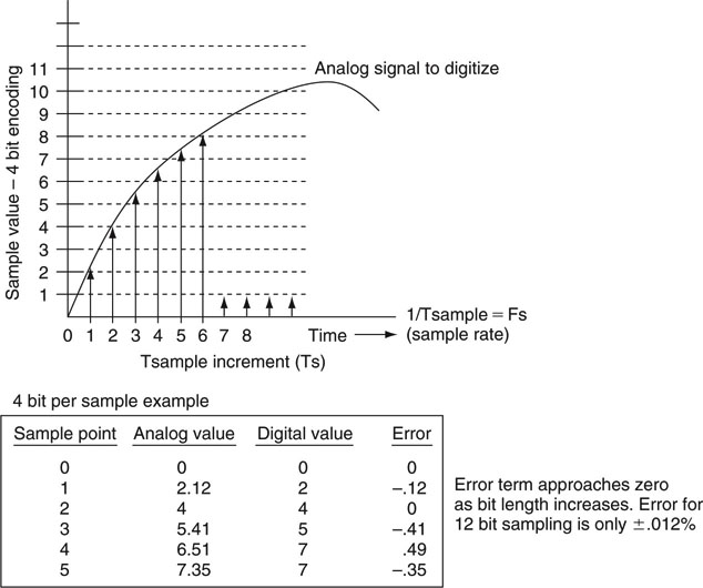
There will always be analog diehards who claim that digital sampling “misses the pieces” between samples. Examining Figure 11.1 may imply this. The famous Nyquist sampling theorem states: “The signal sampling rate must be greater than twice the bandwidth of the signal to perfectly reconstruct the original from the sampled version using the appropriate reconstruction filter.” For example, an audio signal spanning 0 to 20 kHz and sampled at >40 kHz rates (48 or even 96 kHz is typical for professional audio) may be perfectly captured. It is one of those wonderful facts dependent on math and does not sacrifice “missing pieces” in any way.
Okay, there are two “pieces” involved here. One piece is along the horizontal time axis, as snapshot values only occur at sample points. However, according to Nyquist, zero signal fidelity is lost if samples are spaced uniformly at a sufficiently high sample rate. The second piece is along the vertical (voltage) axis. In practice, the vertical domain must be digitized to N-bit precision. For audio signals, a 24-bit (16 and 20 also used) A–D is common, which yields vertical impression that cannot be detected aurally. For video, 12-bit precision is common for some applications, which yields noise that is well below visual acuity. The ubiquitous serial digital interface (SDI) link carries video signals at 10-bit resolution. Admittedly, 10-bit, especially 8-bit, resolution does produce some visual artifacts. Here is some sage signal-flow advice: digitize early, as in the camera, and convert to analog late, as for an audio speaker or not at all as for a flat panel display. Yes, core to AV/IT systems are digital audio and video.
It should be mentioned that capturing an image with a sensor is a complex operation and that it is nearly impossible to avoid some sampling artifacts (aliasing) due to high-frequency image content. With audio, Nyquist sampling yields perfect fidelity, whereas with video there may be some image artifacts due to scanning parameter limitations with “random” image content.
11.2 PROGRESSIVE AND INTERLACE IMAGES
The display of the moving image is part art and part science. Film projects 24 distinct frames usually shuttered twice per frame to create a 48 image per second sequence. The eye acts as a low-pass filter and integrates the action into a continuous stream of images without flicker. Video technology is based on the raster—a “beam” that paints the screen using lines that sweep across and down the display. The common tube-based VGA display uses a progressive raster scan; i.e., one frame is made of a continuous sequence of lines from top to bottom. Most of us are familiar with monitor resolutions such as 800 × 600, 1,024 × 768, and so on. The VGA frame rate is normally 60 or 72 frames per second. Most VGA displays are capable of HD resolutions, albeit with a display size not large enough for the comfortable ~9-foot viewing distance of the living room. By analogy, a digital or film photo camera produces a progressive image, although it is not raster based.
FIGURE 11.2 An interlaced picture frame: First field followed by second field in time and space.
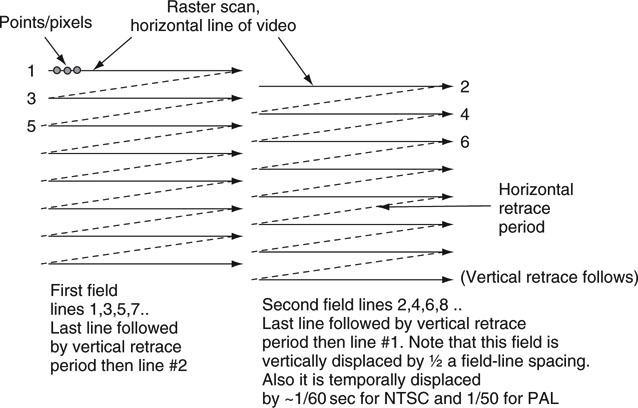
The common analog TV display is based on an interlaced raster. Figure 11.2 illustrates the concept. A frame is made of two fields,1 interleaved together. The NTSC frame rate is 302 frames per second (FPS) and it is 25 for PAL. The second field is displaced from the first in time by 1/60 (or 1/50) second and vertically offset by one-half field-line spacing. Each field has one-half the spatial resolution of the resultant frame for non-moving images. A field is painted from top to bottom and from left to right. Why go to all this trouble? Well, for a few reasons. For one, the eye integrates the 60 (50) field images into a continuous, flicker-free, moving picture without needing the faster frame scan rates of a progressive display. In the early days of TV, building a progressive 60 FPS display was not technically feasible. Second, the two fields combine to give an approximate effective spatial resolution equal to a progressive frame resolution. As a result, interlace is a brilliant compromise among image spatial quality, flicker avoidance, and high scanning rates. It is a form of video compression that saves transmission bandwidth at the cost of introducing artifacts when there is sufficient image motion.
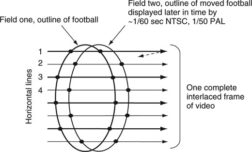
Why does the interlace process introduce motion artifacts? Figure 11.3 shows the outline of a football as it is captured by two successive fields. Each field has half the resolution of the composite frame. Note that the ball has moved between field captures, so horizontal lines #1 and #2 display different moments in time but are adjacent in a spatial sense. A printout of a single frame (a frozen frame) with image motion looks ugly with jagged tears at the image edges. This can be seen in Figure 11.3. Fortunately, the eye is not highly sensitive to this oddity at 60 (50) fields per second. Also, when a captured image has detail on the order of a single display line height, then some obnoxious flicker will occur at the frame rate. With the advent of HD resolutions, both progressive and interlace formats are supported. Progressive frames appear more filmlike and do not exhibit image tearing. With the advent of flat panel displays at 60 and 120 Hz rates, interlaced formats will give way to all things progressive.
FIGURE 11.3 Interlace offsets due to image movement between field scans.
![]() Having trouble remembering the difference between a frame and a field? Think of this: a farmer took a picture of his two fields and framed it. There are two fields displayed in the frame.
Having trouble remembering the difference between a frame and a field? Think of this: a farmer took a picture of his two fields and framed it. There are two fields displayed in the frame.
11.3 VIDEO SIGNAL TIMING
In order to understand the basics of video timing, we have posited an example based on a monochrome (gray scale) signal. Color video signals are considered later, but the same timing principles apply. At each point along a horizontal line of video, the intensity (black to white) is relative to image brightness. To paint the screen either progressively or using an interlaced raster, we need a signal that can convey image brightness along with the timing to trigger the start of a line, the end of a line, and the vertical retrace to the top of the screen. The luma3 signal in Figure 11.4 meets our needs. The luma signal represents the monochrome or lightness component of a scene. The active video portion of a line is sourced from file data, image sensors, computable values, and so on. It is of value to note that most A/V files do not carry horizontal or vertical timing information. Timing must be added by hardware circuitry as needed by the delivery chain.
FIGURE 11.4 Synthesis of a monochrome video signal.
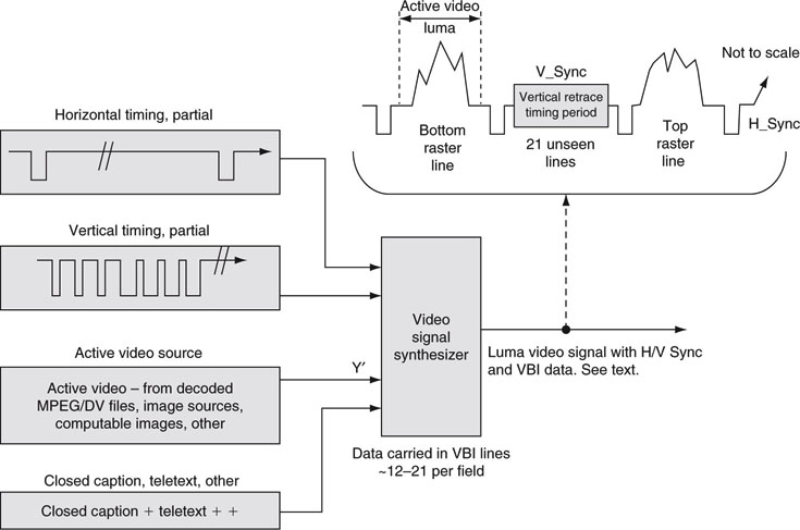
The receiver uses the horizontal timing period to blank the raster during the horizontal beam retrace and start the next line. The receiver uses the vertical timing to retrace the raster to the top of the image and blank the raster from view. The vertical period is about 21 unseen lines per field. Lines −12–21 (of both fields) are often used to carry additional information, such as closed caption text. This period is called the vertical blanking interval (VBI). The vertical synchronizing signal is complex, and all its glory is not shown in Figure 11.4. Its uniqueness allows the receiver to lock onto it in a foolproof way.
11.4 VIDEO RESOLUTIONS AND ASPECT RATIOS
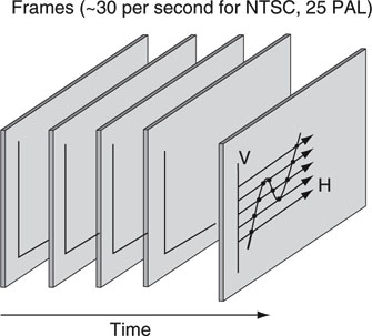
We see a moving 2D image space on the TV or monitor screen, but it requires a 3D4 signal space to produce it. Time is the third dimension needed to create the sensation of motion across frames. Figure 11.5 illustrates a sequence of complete frames (either progressive or interlace). There are four defining parameters for a color digital raster image:
FIGURE 11.5 Video is a 3D spatiotemporal image.
1. Number of discrete horizontal lines—related to the vertical resolution. Not all of the lines are in the viewing window.
2. Number of discrete sample “points” along a horizontal line and bit resolution per point—both related to the horizontal resolution.
• Not all of these points are in the viewing window. Each “point” is composed of three values from the signal set made from R, G, and B values (see Section 11.5).
3. Number of frames per second—related to the temporal resolution. This is–29.97 for NTSC and 25 for PAL, for example.
4. Image aspect ratio—AR is defined as the ratio of the picture width to its height. The traditional AR for analog TVs and some computer monitors is 4 × 3. So-called widescreen, or 16 × 9, is another popular choice.
Next, let us look at the scanning parameters for the standard definition video image. There is a similar set of HD metrics as well, and some are covered in Table 11.1. Figure 11.6 outlines the key measures for a frame of SD video. They are as follows:
Table 11.1 Common SDTV and HDTV Production Scanning Parameters
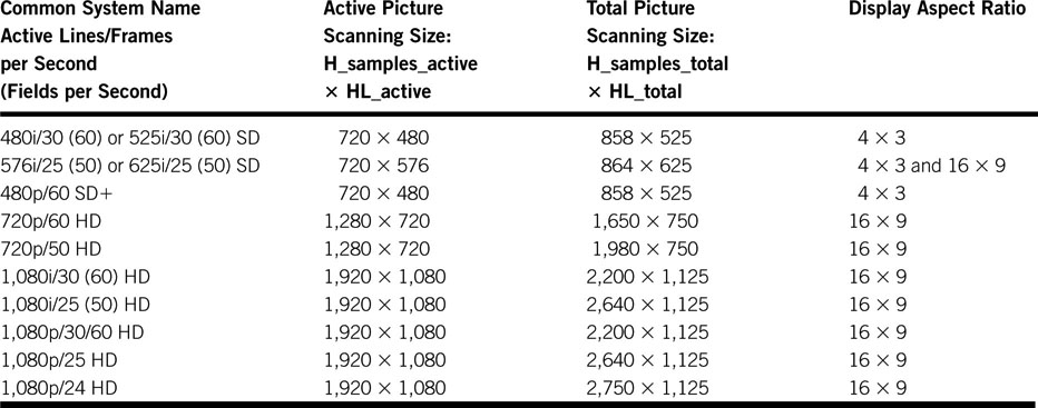
(1) The line count and sample metrics were defined earlier in this section (see Figure 11.6 for SD reference). The “i” term indicates interlace, the “p” indicates progressive scanning. It is common to refer to a 1080i system as either 1080i/30 or 1080i/60; the difference being the reference to frame versus field repeat rates. This reasoning applies to the other interlaced scanning standards as well. The 480p system falls between legacy SD and HD. It has twice the temporal resolution (60 frames per second) of SD formats, but because the horizontal resolution is still 720 points, it will be closed as SD. Each of the frame rates 24, 30, and 60 has an associated system scaled by 1000/1001. NTSC uses the 525/30 system, and PAL uses the 625/25 system. A “point” along the horizontal line is composed of an RGB signal set.
FIGURE 11.6 Image frame sizes and metrics.
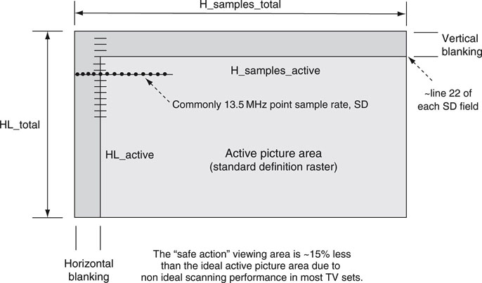
• HL_total—total horizontal lines. For NTSC SD production, this is 525 lines and 625 for PAL.
• HL_active—lines in the active picture area. For NTSC production, this is 480 lines and 576 for PAL. Only these lines are viewable. Usually, the first viewable line starts at the ~22nd line of each field.
• H_samples_total—digital sample points across one entire line, including the horizontal blanking period. There are 858 points (525 line system) and 864 points (625 line system) using a 13.5 MHz sample clock and a 4 × 3 aspect ratio.
• H_samples_active—digital sample points in viewing window. There are 720 active points for 525 and 625 line systems. This is a key metric for video processing and compression.
The horizontal sampling rate for SD production is 13.5 MHz. Other SD rates have been used, but this is widely accepted. For HD resolution, a common sampling rate is ~74.25 MHz. What is the total picture bit rate for an SD, 525, 4 × 3 digital frame? Consider: 525_bit_rate 525 lines × 858 points/line × 3 samples/point × 29.97 FPS 10 bits/sample = 405 Mbps. Another way to get to this same result is 13.5 MHz × 3 samples/point × 10 bits/sample = 405 Mbps.
A common data rate reduction trick in image processing is to reduce the color resolution without adversely affecting the image quality. One widely accepted method to do this, explained in Section 11.5.4, reduces the overall picture bit rate by one-third, which yields a 270 Mbps (= 405 Mbps × 2/3) data rate. This value is a fundamental data rate in professional standard definition digital video systems.
Incidentally, 10 bits per sample is a popular sampling resolution, although other values are sometimes used. Surprisingly, for a 625 (25 FPS, same one-third bit rate reduction applied) system, the total picture bit rate is also exactly 270 Mbps. For HD 1080i/30 video the full frame sample rate is 1.485 Gbps. See Appendix G for more insight into this magic number. Note that this value is not the active picture data rate but the total frame payload per second. The active picture data rate is always less because the vertical and horizontal blanking areas are not part of the viewable picture.
There are a plethora of other video format standards, including one for Ultra High Definition Video (UHDV) with 7,680 × 4,320 pixels supported by a super surroundsound array with 22.2 speakers. An uncompressed 2-hour movie requires ~25TB! Developed by Japan’s NHK, this could appear circa 2016. Digital Cinema and associated production workflows (Digital Intermediate, DI) are often produced in 2 K (2,048 horizontal pixels per line) or even in 4 K (4,096 pixels) formats.
See SMPTE 274M and 296M for details on the sampling structures for HD interlace and progressive image formats.
Most professional gear—cameras, NLE’s video servers, switchers, codecs, graphics compositors, and so on—spec their operational resolutions using one or more of the metrics in Table 11.1. In fact, there are other metrics needed to completely define the total resolution of a video signal, and Section 11.5 digs deeper into this topic.
11.4.1 Aspect Ratio Conversions
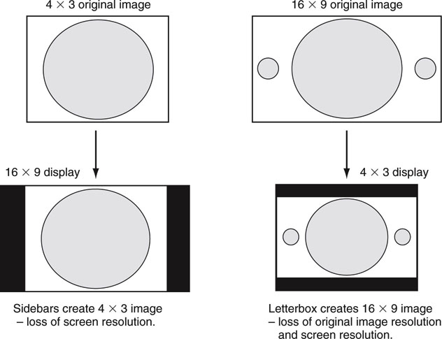
One of the issues with scanning formats is display mapping. Programming produced in 16 9 and displayed on a 4 × 3 display, and vice versa, needs some form of morphing to make it fit. Figure 11.7 shows the most popular methods to map one AR format into another for display. Another method includes panning and scanning the 16 × 9 original image to select the “action areas” that fit into a 4 × 3 space. This is used commonly to convert widescreen movies to 4 × 3 without using letterbox bars. Still another method uses anamorphic squeezing to transform images from one AR to another. This technique always creates some small image distortion, but it utilizes the full-screen viewing area. Whatever the method, AR needs to be managed along the signal chain. Generally, both 16 × 9 and 4 × 3 formats are carried over the same type of video links.
FIGURE 11.7 Common aspect ratio conversions.
11.5 VIDEO SIGNAL REPRESENTATIONS
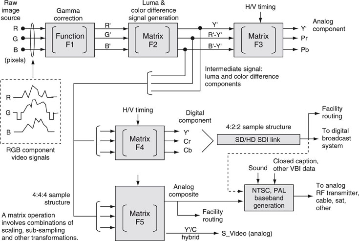
There are many ways to represent a video signal, and each has some advantage in terms of quality or bandwidth in both analog and digital domains. Figure 11.8 outlines eight different signal formats. Figure 11.8 is conceptual, and no distinction is made between SD/HD formats. The H/V timing is loosely applied (or not applied) for concept only. It is not a design specification, but a high schematic level view of these important signal formats. In practice, some of the signals may be derived more directly via other paths, so consider Figure 11.8 as representational of the conversion processes. The matrix Fx term indicates mathematical operations for signal conversion and is different for HD and SD matrix operations. Keep in mind that all the operations are reversible; i.e., R’G’B’ can be recovered for display from, say, Y’CrCb or S_Video, but there is always some loss of fidelity due to the effects of the matrix math. Let us examine each signal and conversion path in Figure 11.8.
FIGURE 11.8 Conceptual view of main video signal representations.
11.5.1 The RGB and R’G’B’ Signals
At the start of the image chain is a camera imager or other means to generate a raw RGB signal. Red, green, and blue represent the three primary color components of the image; 0 percent RGB is pure black and 100 percent is pure white. The signal requires three channels for transport: one per pixel component. The three time-based signals are shown by example in the dotted box, with the green signal having horizontal syncs indicating the start and end of a line. This signal set is rarely used standalone but needs conversion to a gammacorrected version, R’, G’, and B’. Basically, gamma correction applies a power function to each of the three RGB components. The general function (F1) is of the approximate form A’ A0.45, where the 0.45 is a typical gamma value. An apostrophe is used to represent a gamma-corrected signal. According to (Poynton 2003), “Gamma is a mysterious and confusing subject because it involves concepts from four disciplines: physics, perception, photography, and video. In video, gamma is applied at the camera for the dual purposes of precompensating the nonlinearity of the display’s CRT and coding into perceptually uniform space.” Charles Poynton does a masterful job of explaining the beauty of color science, gamma, luma, and chroma, so consult the reference for a world-class tour of these important parameters and much more. For our discussion, gamma correction is an exponential scaling of the RGB voltage levels. In the context of Figure 11.6, each “sample point” refers to the three pixels as a data set.
11.5.2 The Component Color Difference Signals
A full-bandwidth R’G’B’ signal is a bandwidth hog and is used only for the most demanding applications where quality is the main concern (graphics creation, movies, and other high-end productions). Ideally, we want a reduced bandwidth signal set that still maintains most of the RGB image quality. We find this at the next stop in the signal chain: conversion to the Y’, R’-Y’, B’-Y’ signal components. These are not RGB pixels but are derived from them. The Y’ term is the luma signal (gray scale), and the other two are color difference signals often called chroma signals. Interestingly, statistically, 60–70 percent of scene luminance comprises green information. Accounting for this, and removing the “brightness” from the blue and red and scaling properly (matrix F2), yields two color difference signals along with the luma signal. What are the advantages of this signal form? There are several. For one, it requires less data rate to transmit and less storage capacity (compared to R’ G’B’) without a meaningful hit in image quality for most applications. Yes, there is some non-reversible image color detail loss, but the eye is largely insensitive to a high degree due to the nature of F2’s scaling. In fact, there is a loss of 75 percent of the colors when going from an N-bit R’G’B’ to an N-bit color difference format. If N is 8 bits, then some banding artifacts will be seen in either format. At 12 bits, artifacts are imperceptible. Despite the loss of image quality, the transformation to color difference signals is a worthwhile trade-off, as will be shown in a moment. See (Poynton 2003) for more information on this transformation.
Giving a bit more detail, the following conversions are used by matrix F2 for SD systems:
The coding method is slightly different for HD formats, as HD and SD use separately defined colorimetry definitions. Other than this, the principles remain the same.
11.5.3 The Y’PrPb Component Analog Signal
The color difference signals are intermediate forms and are not transported directly but are followed by secondary conversions to create useful and transportable signals. Moving along the signal chain, the Y’PrPb signal set is created by the application of matrix operation F3. Y’PrPb is called the analog component signal, and its application is mainly for legacy use. The P stands for parallel, as it requires three signals to represent a color image. Function F3 simply scales the two chroma input values (R’– Y’ and B’– Y’) to limit their excursions. The Y’ signal (and sometimes all three) has H/V timing, and its form is shown as the middle trace of Figure 11.10.
11.5.4 The Y’CrCb Component Digital Signal
Matrix F4 produces the signal set Y’CrCb, the digital equivalent of Y’PrPb with associated scaling and offsets. The C term refers to chroma. Commonly, each component is digitized to 10-bit precision. This signal is the workhorse in the A/V facility. The three components are multiplexed sequentially and carried by the SDI interface. More on this later. One of the key advantages to this format is the ability to decrease chroma spatial resolution while maintaining image quality, thereby reducing signal storage and data rate requirements. Sometimes this signal is erroneously called YUV, but there is no such format. However, the U and V components are valuable and their usage is explained in Section 11.5.5.
11.5.4.1 Chroma Decimation
The Y’CrCb format allows for clever chroma decimations, thereby saving additional storage and bandwidth resources. In general, signals may be scaled spatially (horizontal and/or vertical) or temporally (frame rates) or decimated (fewer sample points). Let us focus on the last one. A common operation is to decimate the chroma samples but not the luma samples. Significantly, chroma information is less visually important than luminance, so slight decimations have little practical effect for most applications. Notably, chroma-only decimation cannot be done with the RGB format—this is a key advantage of the color difference format.
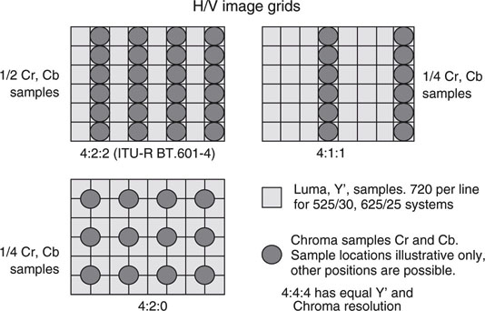
Our industry has developed a short-form notation to describe digital chroma and luma decimation, and the format is A:B:C. The A is the luma horizontal sampling reference, B is the chroma horizontal sampling factor relative to A, and C is the same as B unless it is zero, and then Cr and Cb are subsampled vertically at 2:1 as well. It is confusing at best, so it is better not to look for any deep meaning in this shorthand. Rather, memorize a few of the more common values in daily use. The first digit (A) is relative to the actual luma pixel sample rate, and a value of 4 (undecimated luma) is the most common. Luma decimation, in contrast to chroma decimation, sacrifices some observable image quality for a lower overall bit rate. In most cases, it is the chroma that is decimated, not the luma. Some of the more common notations are as follow.
• 4:4:4—luma and 2 chroma components are sampled equally across H and V.
• 4:2:2—chroma (Cr and Cb) sampled at half of luma rate in the horizontal direction (1/2 chroma lost).
• 4:2:0—chroma sampled at half of luma rate in H and V directions (three-fourths chroma lost). The DV-(625/50) format uses this, for example.
• 4:1:1—chroma sampled at one-quarter of luma rate in the H direction (three-fourths chroma lost). The DV-(525/60) format uses this, for example.
• 3:1:1—as with 4:1:1 except one-fourth of luma samples are also discarded. A 1,920 sample point HD line is luma subsampled to 1,440 samples. Sony HDCAM format, for example.
• 4:4:4:4—the last digit indicates that an alpha channel (transparency signal) is present and sampled at the luma rate.
It turns out that 4:2:0 and 4:1:1 have an equal number of chroma samples per frame, but the samples are at different locations on the grid. Figure 11.9 shows examples of the Y’, Cr, Cb sample grid for different methods. The common SDI studio link normally carries 4:2:2 SD/HD video at 10 bits per sample. Conceptually, the sequential order of carriage over SDI for 4:2:2 samples is Y’ Cr Y’ Cb Y’ Cr Y’ and so on. It is easy to see the one-half Cr and Cb chroma rate compared to the luma rate. For 4:2:0 there are one-half as many chroma samples compared to 4:2:2 and one-fourth compared to 4:4:4 (Y’ Cr Cb Y’ Cr Cb Y’, etc.). In practice, the decimated Cr and Cb samples are derived by averaging several adjacent chroma values from the 4:4:4 signal. This gives a slightly better result than unceremoniously dropping chroma samples from the 4:4:4 source.
FIGURE 11.9 A comparison of chroma sampling in 4:2:2, 4:1:1, and 4:2:0 formats.
The 4:2:2, 4:2:0, and 4:1:1 decimations are used as the source format for many video compression methods, including MPEG and DV. In fact, these codecs get an extra boost of compression when they decimate the chroma before the actual compression starts. Both DVB and ATSC digital transmissions systems utilize 4:2:0 decimated chroma at 8-bit resolution luma and chroma. The 4:4:4 HD R’G’B’ format is used for high-end applications, and a dual-link HD-SDI method (2 × 1.485 Gbps data rate) is defined for carrying the three synchronous signals.
11.5.5 The Analog Composite Video Signal
The analog composite5 video signal is output from matrix F5, as shown in Figure 11.8. This signal is illustrated in Figure 11.10 (top trace). The middle trace is the luma (plus H/V timing) signal. The bottom trace is the chroma signal (plus color burst, explained shortly). The top trace is composed of the sum of the bottom two signals and contains color and brightness information in one signal. A receiver can recover the H/V timing, brightness, and color details from the signal.
FIGURE 11.10 The making of a composite video signal.

Note: These are conceptual diagrams and some details are simplified (not to scale).
The composite signal is a wonderful invention, has a long history of use, and is the basis of the NTSC and PAL analog transmissions systems. Over the past 50 years, most TV stations and A/V facilities have used it as the backbone of their infrastructure, although the digital component SDI link is quickly replacing it. Most consumer A/V gear supports composite I/O as well. Also, there is a digital composite version of this often referred to as a “4Fsc composite,” but it is used infrequently.
So what is the trick for carrying color and luma as one signal? Actually, there are several. First, let us define the U and V signals. Simply, these are scaled versions of the two color difference signals B’– Y’ and R’– Y’, [Eqs. (11.3) and (11.2) (Section 11.5.2)].
If we want to reduce the bandwidth further, U and V are bandwidth filtered and scaled. Next, they are combined into a single color signal, C, by quadrature modulating a subcarrier at frequency F sc.
where6 ω = 2πFsc and F sc is the color subcarrier frequency. C is formed by AM modulating sin(ωT) with U and cos(ωT) with V both at the same frequency Fsc. C is shown as the bottom trace of Figure 11.10 along with the color burst reference signal, explained later.
Fsc is chosen at ~3.58 MHz for NTSC and ~4.43 MHz for most PAL systems. Now, the composite baseband video signal is
When we select the value of the color subcarrier Fsc judiciously, the Y’ and C terms mix like oil and water; they can be carried in the same bucket, but their identity remains distinct. Ideally, a receiver can separate them and, via reverse matrix operations, re-create the R’G’B’ signals ready for display. See again Figure 11.10 and imagine the bottom trace (C) and the middle trace Y’ summed to create the top trace—this is Equation (11.5). In reality, due to a variety of factors, R’G’B’ is not perfectly recovered but close enough in practice. Also, the C component is bandwidth limited by a filter operation before being summed with the luma signal; this limits the chroma resolution slightly.
In order for the receiver to demodulate C and recover U and V, it needs to know precisely the frequency and phase of the subcarrier. The “color burst” is an 8–10 cycle sample of sin(ωT) injected for this purpose.
It is a beautiful technique. See (Jack 2001) and (Poynton 2003) for more details on both composite and component signals and interfacing.
Composite video may be viewed as an early form of video compression. When luma and chroma are combined in clever ways, the bandwidth required to transport and store video is reduced significantly. The composite formulation makes acceptable compromises in image quality and has stood the test of time.
11.5.6 The S_Video Signal
The final signal to discuss is the analog S_Video signal, sometimes called Y/C or YC. This is just signals Y’ and C carried on separate wires. Because there are never any Y’/C mixing effects as may occur in a pure composite signal, R’G’B’ can be recovered with higher fidelity. The burst is carried on the C signal. S_Video is rarely used in professional settings but is a popular SD consumer format.
11.5.7 Analog and Digital Broadcast Standards
All of the video standards reviewed in the preceding sections define baseband signals. These are not directly transmittable without further modification. Figure 11.8 shows the step of adding sound and other ancillary information to form a complete NTSC or PAL baseband signal. For analog broadcasts, the complete signal is upconverted to a RF channel frequency for ultimate reception by a TV. The input to this process may be a composite analog or digital component signal for added quality. Audio modulation uses FM and has a sub-carrier of 4.5 MHz for NTSC. At the receiver, the RF signal is deconstructed and out plops R, G, B, and sound ready for viewing.
Three analog TV transmission systems span the world; they are NTSC, PAL, and SECAM (see the Glossary). Each has variations, with the color burst frequency and total baseband bandwidth being key variables. NTSC/M, J and PAL/B, D, G, H, I, M, N, and various SECAM systems are used worldwide and are adopted on a per country basis. See (Jack 2001) for a complete list of systems and adopted countries.
Before 1953, NTSC only defined B &W visuals with a temporal rate of exactly 30 FPS. When NTSC color was introduced, the committee had a conundrum to handle. If any non-linearity arose in the signal chain, color spectra information, centered approximately at 3.58 MHz (Fsc), and the soundmodulated spectra, centered on 4.5 MHz, may interfere. The resulting intermodulation distortion would be apparent as visual and/or aural artifacts. The problem was avoided by changing the temporal frame rate. This is an overly simplified explanation, but the end result was to apply a scaling factor of 1,000/1,001 to the B &W frame rate. This resulted in a new frame rate of ~29.97 and a corresponding field rate of ~59.94. No big deal it seems. However, this change introduced a timing discrepancy that is a pain to deal with, as the wall clock is now slightly faster than the field rate.
The 1,000/1,001 factor is awkwardly felt when a video signal or file is referenced by time code. Time code assigns a frame number to each video frame, but a ~29.97 FPS rate yields a non-integer number of frames per second. A frame location based on a wall clock requires some time code gymnastics to locate it in the sequence. See Section 11.9 for more information on time code.
11.5.7.1 Digital Broadcast Standards
Analog TV broadcast systems are slowly being replaced with digital transmission systems worldwide. Figure 11.8 shows a SDI signal source feeding a digital broadcast system. There are four systems in general use. In Europe, Digital Video Broadcasting (DVB) standards began development in 1993 and are now implemented by 55+ countries over terrestrial, satellite, and cable. In the United States, the Advanced Television Systems Committee (ATSC) produced its defining documents in 1995 as the basis of the terrestrial DTV system. As of February 17, 2009, all full-power U.S. stations are transmitting using DTV formats. In Japan, the Integrated Services Digital Broadcasting (ISDB) system began life in 1999 and supports terrestrial, satellite, and cable. In China, DMB-T/H is specified with support for MPEG AVC and other compression standards. All four systems offer a selection of SD and HD video resolutions, use MPEG2 compression (or advanced versions), have six-channel surround sound, support non-A/V data streams, and use advanced modulation methods to squeeze the most bits per allocated channel bandwidth. The MPEG Transport Stream (TS) is a common data carrier for these systems. The TS is a multiplexing structure that packages A + V + data into a single bit stream ready for transmission. The TS method has found wide use. Many codecs have a mapping into the TS structure, including the popular H.264 method.
The typical transmitted maximum compressed HD data rate is ~20 Mbps for 1080i/60 programming, although smaller values are common as broadcasters trade off image quality for extra bandwidth to send other programming or data streams. The main A/V program source to the encoding and transmission system is usually SDI or HD-SDI signals. No longer are composite signals used or desired. The new standards create a digital pipe to the viewer, and the broadcaster can use it in a wide variety of ways. The Web is filled with information on digital broadcast standards. See www.atsc.org or www.dvb.org for more information.
11.5.8 Professional Signal Formats—Some Conclusions
How should we rank these signal formats in terms of quality? Well, the purest is R’G’B’, but due to its high bandwidth requirements, it is used only for very high-end A/V applications. The SD/HD Y’CrCb format is the workhorse of most facilities. It provides excellent quality; all components are separate, 4:2:2 resolution, 10 bits per component and all digital. Component video values are easily stored in a file. Plus, audio channels may be multiplexed into the SDI stream, creating an ideal carrier for A/V essence. All analog and composite formats are fading out. There are other formats, for sure, and some are specific to consumer use and others for very high-end HD use. Knowledge of the ones covered in this section will allow you to springboard to other formats with ease.
Figure 11.11 outlines a general selection of common interface standards across analog, digital, and AV/IT systems. Although R’G’B’ is also transported for high-end applications, it is not shown on the diagram. Most digital facilities use SDI links and AES/EBU links to carry A/V signals. The next two sections review these two important links. Together with LAN/WAN, they make up the lion’s share of transport means in a converged AV/IT system.
FIGURE 11.11 Common professional A/V interface standards.
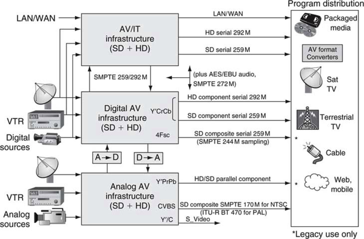
![]() In terms of video quality and transport convenience, digital trumps analog, component formats trump composite, and serial links trump parallel links.
In terms of video quality and transport convenience, digital trumps analog, component formats trump composite, and serial links trump parallel links.
11.6 SDI REVIEW—THE UBIQUITOUS A/V DIGITAL LINK
The serial digital interface (SMPTE 259M for SD, 292M for HD) link has revolutionized the digital A/V facility. It has largely replaced the older analog composite link and digital parallel links, so it is worth considering this link for a moment to fully appreciate its power within the digital facility. SDI supports component video (Y’CrCb) SD and HD formats (supporting a variety of frame rate standards). The typical SD line bit rate is 270 Mbps (with support from 143 to 360 Mbps depending on the data format carriage) and is designed for point-to-point, unidirectional connections (see Appendix G).
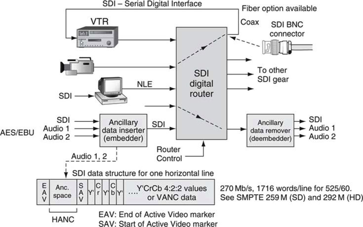
SDI is not routable in the LAN/IP sense; however, an entire industry has been created to circuit switch SDI signals using video routers. Due to non-displayable areas in the raster scan, the active image data payload is less than the link rate of 270 Mbps. For example, the actual active picture data payload of a 525-line, 10 bits/pixel, 4:2:2 component signal is ~207.2 Mbps, not counting the vertical and horizontal blanking areas. Figure 11.12 shows the basic framing structure of a SDI signal and an example of SDI link routing. Routers range in size from a basic 8 × 1 to mammoth 512 × 512 I/O and larger. About 57 Mbps out of the total of 270 is available to carry non-video payloads, including audio. These nonvideo data are carried in both horizontal ancillary (HANC) and vertical ancillary (VANC) blanking areas. In a non-picture line, data between SAV and EAV markers carry ancillary VANC data.
FIGURE 11.12 Basic SDI use and framing data structure.
Examples of payloads that SDI can carry are as follows:
• SD video with embedded digital audio. One channel of video and eight embedded uncompressed stereo pairs (16 audio channels) are a supported payload.
• Ancillary data carried in HANC and VANC areas. SMPTE has standardized several schemes for HANC and VANC non-video data carriage.
• Carriage of compressed formats in the SDTI-CP wrapper. SDTI-CP (Serial Digital Transport Interface—Content Package) is a means to carry compressed formats such as MPEG and DV over SDI links. This method was popularized by Sony’s IMX digital MPEG VTR and Panasonic’s DVCPro VTRs. See SMPTE standards 326M and 331M for more information.
• HD-SDI (SMPTE 292M) uses a line bit rate 5.5 times higher than that of 259M (270 Mbps typical), clocking in at 1.485 Gbps to carry uncompressed HD video, embedded audio, and ancillary data.
• At the high end of production standards, SMPTE defines the 424M/425M serial link for carrying 1,080p/60 video at 3 Gbps. Also, SMPTE 435 defines a 10 Gbps (actually 10.692 nominal) link for carry ing a 12 bits/pixel, 4:4:4, RGB format and other common formats in multiplexed style.
There is no H/V timing waveform embedded in a digital SDI link as with the analog luma or composite video signal. Rather, timing is marked using SAV, EAV words, and other sync words. These markers may be used to help create H/V timing as needed. Most professional AV/IT systems will be composed of a mix of SDI, HD-SDI, AES/EBU audio, and LAN/WAN links. The workhorse for audio is the AES/EBU link discussed next.
11.6.1 The AES/EBU Audio Link
The AES/EBU (officially AES3) audio standard defines the data structures and physical serial link to stream professional digital audio. It came about as a result of collaboration between the AES and the EBU and was later adopted by ANSI. The default AES/EBU uncompressed sample rate is 48 kHz, although 44.1, 96 kHz and others are also supported. An audio sample accuracy of 24 bits/sample (per channel) is supported, but not all equipment will use the full 24 bits. Most devices use 16 or 20 bits per sample. A full frame is 32 bits, but 8 bits of this are dedicated to non-audio user bits and synchronization.
A shielded, twisted-pair cable with XLR connectors on both ends is used to transfer two channels of audio and other data using a line data rate of about 3 Mbps for 48 kHz sampling. There is also a version that uses coax cable with BNC connectors. Both versions are in wide use. The link also supports a raw data mode for custom payloads. One example of this is the transport of compressed AC3 × 5.1 and Dolby-E audio formats. The AES/EBU data structure may be embedded into a SDI stream for the convenience of carrying up to 16 audio channels and video on one cable (see Figure 11.12).
11.6.2 The Proteus Clip Server Example
Announcing the new—drum roll, please—Proteus clip server: the newest IT-friendly video server with the ability to record (one channel in) and play back (two channels out) A/V files using networked storage. Okay, Figure 11.13 is fictional, but it exemplifies an AV/IT device with a respectable quota of rear panel I/O connectors. A little inspection reveals SDI video I/O (BNC connectors), AES/EBU audio I/O (XLR connector version), time code signal in, a Gen Lock input, an analog signal output using Y’PrPb ports, composite monitoring ports, and a LAN connection for access to storage/files, management processes, device control, and other network-related functions.
FIGURE 11.13 The Proteus clip server: Rear panel view.

The Gen Lock input signal (sometimes called video reference) is a super clean video source with black active video or possibly color bars. The Proteus server extracts the H/V timing information from the Gen Lock signal and uses this to perfectly align all outputs with the same H/V timing. Most A/V facilities use a common Gen Lock signal distributed to all devices. This assures that all video signals are H/V synced. Alignment is needed to assure clean switching and proper mixing of video signals. Imagine cross fading between two video signals each with different H/V timing; the resultant hodgepodge is illegal video. Sometimes it is unavoidable that video signals are out of sync. The services of a “frame sync” are used to align signals to a master video reference (see Appendix B).
Remember too that SDI signals may carry embedded audio channels on both inputs and outputs. Also, the SDI-In signal has a loop-through port. The input signal is repeated to the second port for routing convenience.
11.7 VIDEO SIGNAL PROCESSING AND ITS APPLICATIONS
Video is a signal with 3D spatiotemporal resolutions and has traditionally been processed using hardware means. With the advent of real-time software processing, hardware is playing a smaller role but still finds a place, especially for HD rates. Image handling may be split into two camps: raw image generation and image processing. The first is about the creation and synthesis of original images, whereas the second is about the processing of existing images. Of course, audio signal processing is also of value and widely used, but it will not be discussed here. Image processing is a weighty subject, but let us peek at a few of the more common operations.
1. Two- and three-dimensional effects, video keying, compositing ope rations, and video parameter adjustments
2. Interlaced to progressive conversion—deinterlacing
3. Standards conversion (converting from one set of H, V, T spatiotemporal samples to another set)
4. Linear and non-linear filtering (e.g., low-pass filtering)
5. Motion analysis, tracking (track an object across frames, used by MPEG)
6. Feature detection (find an object in a frame)
7. Noise reduction (reduce the noise across video time, 3D filtering)
8. Compressed domain processing (image manipulation using compressed values)
These operators are used by many video devices in everyday use. The first three deserve special mention. Item #1 is the workhorse of the video delivery chain. Graphics products from a number of vendors can overlay moving 2D and 3D fonts onto live video, squeeze back images, composite animated images, transition to other sources, and more. Video editors apply 2D/3D effects of all manner during program editing. Real-time software-based processing has reached amazing levels for both SD and some HD effects operators. Video parameter adjustments of color, contrast, and brightness are run of the mill for most devices.
Video keying adds a bit of magic to the nightly TV news weather report. A “key” is a video signal used to “cut a hole” in a second video to allow for insertion of a third video signal (the fill) into that hole. Keying places the weather map (the fill) behind the presenter who stands in front of a blue/green screen. The solid color background is used to create the key signal. Keying without edge effects is a science, and video processing techniques are required for quality results.
11.7.1 Interlace to Progressive Conversion—Deinterlacing
Recall that an interlaced image is composed of two woven fields, with the second one being time shifted compared to the first. Each field has half the spatial resolution of the complete frame as a first-order approximation. If the scene has object motion, the second field’s object will be displaced. Figure 11.3 shows the “tearing” between fields due to object displacement. Fortunately, the brain perceives an interlaced picture with a common amount of interfield image motion just fine. However, to print a single interlaced frame without obvious tearing artifacts or to convert between scanning formats, we often need to translate the image to a progressive one. This process is referred to as deinterlacing, as the woven nature of interlace is, in effect, unwoven. Ideally, the resulting progressive video imagery should have no interlaced artifact echoes. Unfortunately, this is rarely the case.
So what methods are used to unweave an interlaced image? A poor man’s converter may brute-force replicate or average select lines, fields, or frames to create the new image. These are not sophisticated techniques and often yield poor results. For example, Figure 11.14 (top) shows an interlaced image frame with field tearing. The bottom left image in Figure 11.14 is a converted progressive image using simple same-field line doubling. It is obvious that the spatial resolution has been cut in half.
FIGURE 11.14 Interlaced to progressive conversion examples.
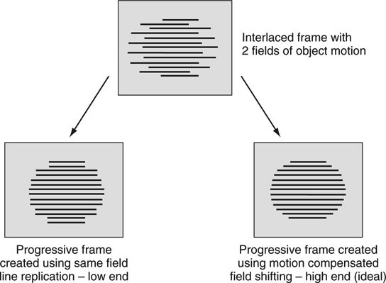
At the high end of performance, motion-compensated deinterlacing measures the field-to-field motion and then aligns pixels between the two video fields to maximize the vertical frame resolution. The lower right image in Figure 11.14 illustrates an ideally deinterlaced image. There are countless variations on these themes for eking out the best conversion quality, but none guarantee perfect conversion under all circumstances. See (Biswas 2003) for a good summary of the methods.
11.7.2 Standards Conversion
The news department just received a breaking story in the PAL video format. It needs to be broadcast immediately over a NTSC system. Unfortunately, the two scanning standards are incompatible. Converting from one H/V/T scanning format to a second H/V/T format is a particularly vexing problem for video engineers (item #3 in the list given earlier). Translating the 25-frame PAL story to a 30-frame NTSC video sequence requires advanced video processing. This operation is sometimes referred to as a “standards conversion” because there is conversion between two different video-scanning standards. The PAL/NTSC conversion requires 5 new frames be manufactured per second along with per frame H/V resizing. Where will these new frames come from? Select lines, fields, or frames may be replicated or judiciously averaged to create the new 30 FPS video. Using motion tracking with line interpolation, new frames may be created with image positioning averaged between adjacent frames.
Reviewing Table 11.1, we see 10 different standards (plus the 1,000/1,001 rate variations) for a total of 15 distinct types. There are 210 different combinations of bidirectional conversions just for this short list. Yes, image-processing algorithms and implementation are becoming more important as scanning standards proliferate worldwide. In widespread use are SD-to-HD upconversion and HD-to-SD downconversion products. Several vendors offer standards converter products.
11.7.3 Compressed Domain Processing
Before leaving the theme of video processing, let us look at item #8 in the list given earlier: the hot topic of compressed domain processing (CDP). Video compression is covered in the next section, but the basic idea is to squeeze out any image redundancy, thereby reducing the bit rate. It is not uncommon for facilities to record, store, and play out raw MPEG streams. However, working natively with MPEG and manipulating its core images are not easy. For example, the classic way for a TV station to add a flood watch warning message to the bottom of a MPEG broadcast video is to decode the MPEG source, composite the warning message, and then recode the new picture to MPEG. This flow adds another generation of encoding and introduces an image quality hit—often unacceptable. With CDP, there is no or very little quality hit in order to add the message. It is inserted directly into the MPEG data stream using complex algorithms that modify only the new overlay portion of the compressed image.
This is an overly simplified explanation for sure, but the bottom line is CDP is a powerful way to enhance MPEG streams at cable head ends and other passthrough locations. Several vendors are offering products with graphical insert (e.g., a logo) functions. Predictably, video squeeze backs and other operations will be available in a matter of time. Watch this space!
Well, that is the 1,000-foot view of some common video processing applications and tricks. Moving on, if there is any one technology that has revolutionized A/V, it is compression. The next section outlines the main methods used to substantially reduce A/V file and stream bit rates.
11.8 A/V BIT RATE REDUCTION TECHNIQUES
The data structures in a digital A/V system are many and varied. In addition to uncompressed video, there are several forms of scaled and compressed video. The following four categories help define the space:
1. Uncompressed A/V signals
2. Scaled uncompressed video in H/V/T dimensions, luma decimation, chroma decimation—lossy
3. Lossless compressed A/V
4. Lossy compressed A/V
Uncompressed video is a data hog from a bandwidth and storage perspective. For example, top-end, raw digital cinema resolution is ~4 K × 2 K pixels, 24 FPS, yielding ~7 Gbps data rate. A standard definition 4:4:4 R’G’B’ signal has an active picture area bit rate of ~311 Mbps. It is no wonder that researchers are always looking for ways to reduce the bit rate yet maintain image quality. Methods #2, #3, and #4 in the preceding list are bit rate reduction methods and are broadly rated against image quality in Figure 11.15. To better understand Figure 11.15, we need to define the term lossy.
FIGURE 11.15 Video data rate reduction examples.
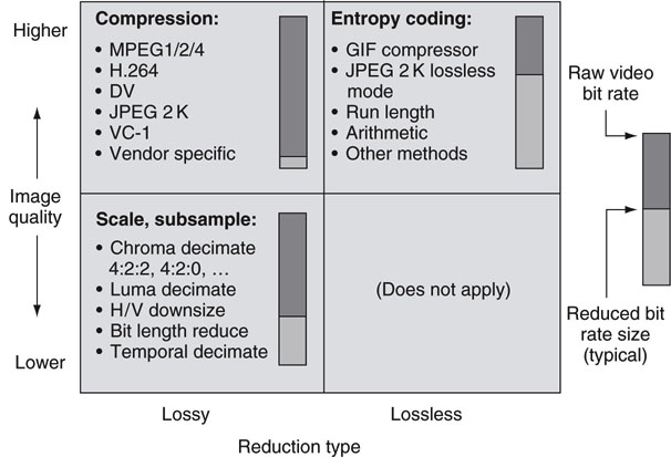
Lossy, in contrast to lossless, is used to describe bit rate reduction methods that remove image structure in such a way that it can never be recovered. This may sound evil, but it is a good trick if the amount of image degradation is acceptable for business or artistic purposes. The lower left quadrant of Figure 11.15 rates quality versus bit reduction for method #2 given earlier. Chroma decimation is generally kind to the image and was discussed in Section 11.5.4. If luma decimation is used, it is much easier to notice artifacts. H/V scaling is done to reduce overall image size. For example, scaling an image to H/2 × V/2 saves an additional factor of 4 in bit rate, but the image size is also cut by 4. Another trick is to brute-force reduce the Y’CrCb bit length per component, say from 10 to 8 bits. This causes some visual banding artifacts in areas of low contrast. The last knob to tweak is frame rate. Reducing it saves a proportional amount of bits; keep going and the image gets the jitters.
The bit rate meter for this method shows a typical 3:1 savings for a modest application of scaling and decimation with virtually no loss of visual quality. Although these methods reduce bit rate, they are not classed as video compression methods. True compression techniques rely on mathematical cleverness, not just brute-force pixel dropping.
The next trick in the bit rate reduction toolbox is shown in the upper right quadrant of Figure 11.15. Lossless encoding squeezes out image redundancies, without sacrificing any quality. This class of rate reduction is called entropy coding after the idea that bit orderliness (low entropy) can be detected and coded with fewer bits. A good example of this is the common GIF still-image file compressor. It is based on the famous Lempel-Ziv-Welch (LZW) algorithm. GIF is not ideal for video but is the basis for similar methods that are applied to video. JPEG 2000 (JPEG2K) has a lossless mode supporting up to 12 bits/pixel encoding, resulting in outstanding quality. Run length coding is employed by MPEG encoders and other compressors to condense strings of repeating digits. Arithmetic coding is used by the H.264 video compressor and others to further pinch down the data rate by locating and squeezing out longer term value orderliness. Most lossless coders achieve bit savings in the 25–50 percent range, but the results are strongly content dependent.
There is no guarantee that a pure lossless encoder will find redundancies, so the worst-case reduction factor may be zero. For example, losslessly coding a video of pure noise results in a bigger file due to coding overhead. As a result, in practice standalone lossless video coders are not common. However, lossless techniques are used liberally by traditional lossy video compressors (the upper left quadrant of Figure 11.15). A lossy compressor uses lossless techniques to gain a smidgen more of overall efficiency.
The real winner in bit rate reduction is true video compression (upper left quadrant of Figure 11.15). It has the potential to squeeze out a factor of ~100 with passable image quality. Consumer satellite and digital cable systems compress some SD channels to ~2.5 Mbps and exceed the 100:1 ratio of savings. Web video compression ratios reach >1,000:1 but the quality loss is obvious. To get these big ratios, compressors use a combination of scaling, decimation, and lossy encoding.
However, some studio-quality codecs compress by factors as small as 3–6 with virtually lossless quality. A 20:1 reduction factor yields a ~15 Mbps SD signal, which provides excellent quality for many TV station and A/V facility operations. Video compression is discussed in Section 11.8.2, but first let us look at some notes on audio bit rate reduction.
11.8.1 Audio Bit Rate Reduction Techniques
The four quadrants of Figure 11.15 have corresponding examples for audio bit rate reduction. Uncompressed audio formats are commonly based on the 16/20/24 bit AES/EBU (3.072 Mbps per stereo pair, including overhead bits) format or BWAV format.
The EBU’s Broadcast WAV format is a professional version of the ubiquitous WAV sound file format but contains additional time stamp and sync information. Lossless audio encoding is supported by the MPEG4 ALS standard, but it is not commonly used. One form of audio scaling reduces the upper end frequency limit, which enables a lower digital sample rate with a consequent bit rate reduction. This is a widespread practice in non-professional settings. Finally, audio compression is used in all forms of commercial distribution and some production. (Bosi 2002) gives a good overview of audio encoding and associated standards, including MP3, AAC, AC3, and other household names. These are distribution formats for the most part. Dolby-E is used in professional settings where quality is paramount. However, let us concentrate on video compression for the remainder of the discussion.
11.8.2 Video Compression Overview
When it comes to compression, one man’s redundancy is another man’s visual artifact, so the debate will always continue as to how much and what kind of compression is needed to preserve the original material. There are three general classes of compression usage. At the top end are the program producers. Many in this class want the best possible quality and usually compress very lightly (slight bit rate reduction) or not at all. Long-term archive formats are often at high-quality levels. The next class relates to content distribution. In this area, program producers distribute materials to other partners and users. For example, network TV evening newscasts are sent to local affiliates using satellite means and compressed video. The level of compression needs to be kept reasonably high and is often referred to as mezzanine compression. Typically, HD MPEG2 programming sent at mezzanine rates range from 35 to 65 Mbps encoded bit rates. The third class is end-user consumption quality. This ranges from Web video at ~250 Kbps to SD-DVD at <10 Mbps to HDTV at 15–20 Mbps to digital cinema at <250 Mbps.
Figure 11.16 shows the landscape of the most common (there are many more) video compression formats in use. Why so many? Well, some are proprietary, whereas others are standardized. Some are designed for SD only, some for HD only, and some are both. A few are defined as a videotape and compression format, and some are improvements in a long line of formats. For example, MPEG1 begat MPEG2, which begat MPEG4, which begat MPEG4 part 10 (same as H.264, ITU-T spec, also called AVC, Advanced Video Codec). In Figure 11.16, the approximate maximum compressed data rate is given alongside each format box; the values are only a general guide. As a common rule, the compressors accept 8 bits of video component in the Y’CrCb format. However, several of the HD formats support 10-bit encoding. The fidelity range extensions (FRExt) of H.264 support encoding rates up to ~1 Gbps for very high-end cinema productions. Most encoders apply some form of chroma and/or luma decimation before the actual compression begins. The compressors in Figure 11.16 are video-only formats for the most part. Audio encoding is treated separately.
FIGURE 11.16 Popular compressed video formats.
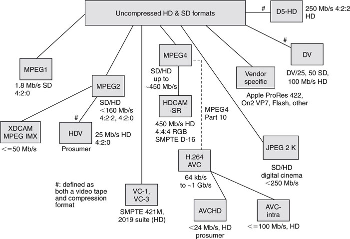
Many of these formats are used in professional portable video cameras and/or tape decks. As such, many are editable and supported by video servers for playback. Most cameras in 2009 capture video on optical disk, HDD, or Flash memory, and 32 and 64 GB Flash cartridges are common. Moving forward, and as memory cost drops, Flash has the edge in terms of high recording rates, fast offload rates, ruggedness, and small size.
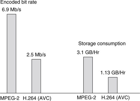
Figure 11.17 compares legacy MPEG2 against H.264 coding efficiency for the same SD source material (Sullivan 2004). This test demonstrates the superiority of H.264 for both bandwidth and storage usage. Here, we see an improvement of 2.75:1 for H.264, although this ratio is a function of source material; it is not a constant. Expect to see satellite TV, cable, and Telco operators (IPTV) using H.264 in their next generation of program delivery.
FIGURE 11.17 Comparing codec efficiencies.
A best practice is to encode strictly and decode tolerantly. What does this mean? When encoding video strictly, apply to the standard in terms of what is legal. When decoding video, apply loosely to the standard. Of course, devices should decode materials that have been strictly encoded but also decode materials that may have deviated from the standard. If possible, rarely terminate a decode session (or generate useless video) based on some out-of-spec parameter. Decoders that do their best are always well respected.
11.8.3 Summary of Lossy Video Compression Techniques
In general, there are two main classes of lossy compression: intraframe and interframe coding. Intraframe coding processes each frame of video as standalone and independent from past or future frames. This allows single frames to be edited, spliced, manipulated, and accessed without reference to adjacent frames. It is often used for production and videotape (e.g., DV) formats. However, interframe coding relies on exploiting temporal redundancies between frames to reduce the overall bit rate. Coding frame # N is done more efficiently using information from neighboring frames. Utilizing frame redundancies can squeeze a factor of two to three better compression compared to intra-only coding. For this reason, the DVD video format and ATSC/DVB transmission systems rely on intraframe coding compression. As might be imagined, editing and splicing interframes are thorny problems due to their interdependencies. Think of interformats as offering more quality per bit than intraformats.
Figure 11.18 illustrates a snapshot of common commercial video formats segregated according to type. This is representative of common formats in use, but not all methods are listed. Intraformats are sometimes called I frame only, signifying that only intraframes are coded.
FIGURE 11.18 Snapshot of compression methods and coding formats.
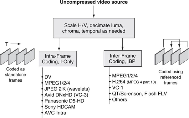
Interformats are sometimes called IBP or long GOP (group of pictures), indicating the temporal association of the compression. The IBP and GOP concepts are described in short order. Note that some I frame-only formats such as JPEG 2000 and DV use only the intramode, whereas others such as MPEG are designed for either mode. In general, interformat compressors can also work in intramode when required. JPEG2K is unique because it has modes for both still picture and video compression. When a JPEG format codes video, it is sometimes called Motion-JPEG.
11.8.3.1 Intraframe Compression Techniques
Squeezing out image redundancies begs the question, “What is an image redundancy?” Researchers use principles from visual psychophysics to design compressors. They learn which image structures are discardable (redundant) and which are not without sacrificing quality. Despite it’s rather Zen-sounding name, visual psychophysics is hardcore science. It examines the eye/brain ability to detect contrast, brightness, and color and to make judgments about motion, size, distance, and depth. A good compressor reduces the bit rate with corresponding small losses—undetectable ideally—in quality.
Of all the parameters, reducing high-frequency detail and chroma decimation reap the most bit savings while maintaining image integrity. These techniques remove the spatial redundancy from the image. Scaling luma or reducing frame rates is usually bad business, and quality drops off suddenly. Figure 11.19 outlines the processes (ignore the second, temporal step for the moment) needed to compress an intraframe video sequence. Each process contributes a portion of the overall compressed bit savings. The order of compression is as follows:
FIGURE 11.19 The basic encoding and decoding processes.
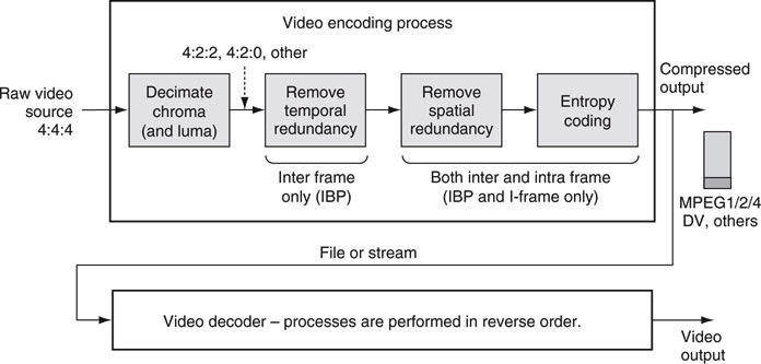
• Decimate chroma and luma in some cases. This provides a lossy bit savings of 50 percent for 4:2:0 scaling.
• Remove high-frequency spatial detail using a filter-like operator and quantize the result. This step saves as much as needed. Pushing this lossy step too far results in obvious visual artifacts.
• Code for lossless entropy. This step saves an additional 30 percent on average.
For the middle step, two methods take the lead: transform based (discrete cosine transform, or DCT) and wavelet based. Both are filter-like operations for reducing or eliminating higher frequency image terms, thus shrinking the encoded bit rate. High-frequency terms arise due to lots of image structure. For example, a close-up image of a plot of grass has significantly more high-frequency terms than, say, an image of a blue wall. The DCT-based filter is used by nearly all modern video compressors. JPEG2K is one major exception; it uses the wavelet method. Mountains have been written about spatial compressing methods. For good overviews, see (Bhaskaran 1997), (Symes 2003), or (Watkinson 2004).
THE DCT IN ACTION 
The DCT is a mathematical device used to transform small pieces of the image domain into an approximation of their frequency domain representation. Once transformed, high-frequency spatial terms can be zeroed out. Plus, other significant spectral lines are quantized to reduce their bit consumption—these steps are lossy. The DCT is tiled across an image frame repeatedly until all its parts have been processed. The resulting terms are entropy encoded and become the “compressed image bit stream.” At the decoder, an inverse DCT is preformed, and the image domain is restored, albeit with some loss of resolution.
Intraframe methods encode each video frame in isolation with no regard to neighboring frames. Most video sequences have significant frame-to-frame redundancies, and intramethods do not take advantage of this; enter interframe encoding.
11.8.3.2 Interframe Compression Techniques
Interframe compression exploits the similarities between adjacent frames, known as temporal redundancy, to further squeeze out the bits. Consider the talking head of a newscaster. How much does the head move from one video frame to the next? The idea is to track image motion from frame to frame and use this information to code more intelligently.
In a nutshell, the encoder tracks the motion of a block of pixels between frames using motion estimation and settles on the best match it can find. The new location is coded with motion vectors. The tracked pixel block will almost always have some residual prediction errors from the ideal, and these are computed (motion compensation). The encoder’s motion vectors and compressed prediction errors (lossy step) are packaged into the final compressed file or stream.
The decoder uses the received motion vectors and prediction errors and recreates the moved pixel block exactly—minus the loss when the error terms were compressed. Review Figure 11.19 and note the “remove temporal redundancy” step for interframe coding.
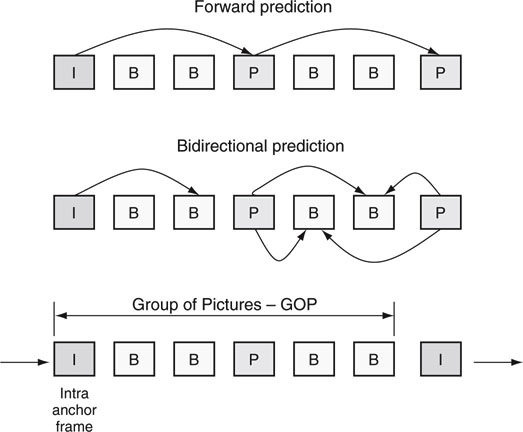
Various algorithms have been invented to track pixel group motion—not necessarily discernible objects. This step is one of the most computationally intensive for an encoding process. This form of encoding is sometimes referred to as IBP or long GOP encoding (see Figure 11.20). A GOP is a sequence of related pictures, usually from 12 to 15 frames in length for SD materials. Here, the I frame is a standalone anchor intraframe. It is coded without reference to any neighboring frames. The B frame is predicted bidirectionally from one or two of its I or P neighbors. A B frame has fewer coded bits than an I frame. The P frame is a forward-predicted frame from the last anchor frame (I or P) and has more bits than a B frame but fewer than an I frame.7 Note that a B or P frame is not the poorer cousin of an I frame. In effect, all frames carry approximately equal image quality due to the clever use of motion estimation and compensation.
FIGURE 11.20 Interframe sequencing examples.
Most MPEG encoders use interframe techniques, but they can also be configured to encode using only intraframe methods. Users trade off better compression efficiency against easy editing, splicing, and frame manipulation when choosing between IBP and I-only formats. A general rule of thumb for production-quality compression is that IBP formats use about 3–4 times fewer bits compared to a pure I-only encoding. For example, an I-only VC-3 encoding at 140 Mbps has about the same visual quality as the Sony XDCAM HD 50 Mbps IBP format.
Researchers are constantly looking for ways to improve compression efficiency, and the future looks bright for yet another round of codecs. In fact, initial work has begun on the tentative H.265 compressor, which holds out the promise of another ~50 percent bit rate reduction within 4 to 5 years.
11.9 VIDEO TIME CODE BASICS
Last but not least is the concept of time code. This “code” is used to link each frame of video to a time value. The common home VCR and DVD use displayed time code to show the progress of a program. The format for professional time code is HH:MM:SS:FF, where H is the hours value (00 to 23), M is the minutes value, S is the seconds value, and F is the frame value (00 to 29 for 525i). A time code of 01:12:30:15 indicates the position of the video at 1 hr, 12 min, 30 s, and 15 frames. If the first frame of the video is marked 00:00:00:00, then 01:12:30:15 is the actual running time to this point. A time code rollover example of 01:33:58:29 is followed by 01:33:59:00.
Accurate A/V timing is the lifeblood for most media facilities. For example, time code is indispensable when queuing up a VTR or video server to a given start point. NLEs use time code to locate and annotate edit points. At a TV station, program and commercial playback is strictly controlled by a playout schedule tied to time code values for every second of the day. SMPTE 12M defines two types of time code: linear (also called longitudinal) time code (LTC) and vertical interval time code (VITC). LTC is a simple digital stream representing the current time code value along with some additional bits. Historically, the LTC low-bit rate format is carried by a spare audio track on the videotape. VITC is a scheme in which time code bits are carried in the vertical blanking interval of the video. This convenient scheme allows the time code to always travel with the video signal and is readable even when the video is in pause mode. In both cases, the time code display format is the same.
Although LTC and VITC were designed with videotape in mind, non-tapebased devices (video servers) often support one or both formats. Time code is carried throughout a facility using an audio cable with XLR connectors. Many vendors offer time code generators that source LTC referenced to a GPS clock. As a result, it is possible to frame accurately sync videos from different parts of a campus or venue and guarantee they are referenced to a common time code value.
11.9.1 Drop Frame Time Code
With 25 FPS video (625i) there is an integer number of frames per second. However, the 525i frame rate is ~29.97 FPS (see Section 11.5.7), and there is not an integer number of frames per second. Standard time code runs exactly 30 FPS for 525i video. A time code rate of 30 FPS instead of ~29.97 creates a 3.6 s error (an extra 108 video frames) every 60 min. This is light years in video time, so we need a way to correct for this. One way to effectively slow down the 30 FPS time code signal is by skipping one time code value every 33.3333 s. This amounts to dropping 108 code points per hour. Now, the 30 FPS time code signal appears to run at ~29.97 FPS. In reality, this is accomplished by dropping frame code numbers 00:00 and 00:01 at the beginning of every minute except for every 10th minute.
Importantly, no actual video frames are dropped, only the time code sequence is modified. If all this is confusing, at least remember that there are two forms of time code: drop frame and non-drop frame. In the 525i/29.97 world, drop frame is popular, whereas in the 625i/25 world, non-drop frame is popular. With 25 FPS material, there is no need to play tricks with the time code values.
Looking ahead, SMPTE is developing a new time code system using a Time Related Label (TRL). The TRL contains the time code field plus additional information (either implicit or easily computable), including frame count from start of material, instantaneous frame rate (FPS), date, and time of day (TOD). The new time label will eventually replace the current bare bones time code field specified by SMPTE 12M. In addition, the overall solution will replace existing methods to synchronize A/V signals across devices and geographies.
11.10 IT’S A WRAP—SOME FINAL WORDS
With this brief overview, you should be conversant with the basics of A/V technology. These themes form the quilt that touches most aspects of professional A/V systems. A key thesis in this book is leveraging IT to move A/V systems to new heights of performance, reliability, and flexibility. By applying the lessons learned in this chapter, plus lessons from the others, you should be well equipped to understand, evaluate, and forecast trends in the new world of converged AV/IT systems.
1 In practice, field lines are numbered sequentially across both fields. To simplify explanations, however, they are numbered as odd and even in Figures 11.2 and 11.3.
2 The frame rate of a NTSC signal is ~29.97 frames per second, and the field rate is ~59.94 fields per second. These strange values are explained later in this chapter. However, for simplicity, these values are often rounded in the text to 30 and 60, respectively. The PAL field rate is exactly 50, and the frame rate is 25 FPS. SECAM uses PAL production parameters and will not be explored further.
3 Technically, only the active picture portion of the signal is the luma value. However, for ease of description, let us call the entire signal luma. Luma (Y´) and chroma are discussed in Section 11.5.
4 Video has the signal dimensions of horizontal, vertical, and time (HVT), so it may be called a 3D signal. Do not confuse this with a moving stereoscopic 3D image, which is a 4D signal.
5 CVBS, composite video burst and sync, is shorthand used to describe a composite signal.
6 The sine sin(w T) term generates a pure single wave at frequency Fsc. The cosine cos(w T) term generates a wave at the same location but shifted by 90 °. The resultant signal C can be demodulated with U and V recovered.
7 These are general IBP bit rate allocations and may differ depending on image content.
REFERENCES
Bhaskaran, V., et al. (1997). Image and Video Compression Standards (2nd edition): Kluwer Press.
Biswas, M., & Nguyen, T. (May 2003). A Novel De-Interlacing Technique Based on Phase Plane Correlation Motion Estimation: ISCAS, http://videoprocessing.ucsd.edu/~mainak/pdf_files/asilomar.pdf.
Bosi, M., Goldberg, R. E., & Chiariglione, L. (2002). Introduction to Digital Audio Coding and Standards: Kluwer Press.
Jack, K. (2001). Video Demystified, A Handbook for the Digital Engineer (3rd edition): Newnes.
Poynton, C. (2003). Digital Video and HDTV, Algorithms and Interfaces. NYC, NY: Morgan Kaufmann.
Sullivan, G. J., et al. (August 2004). The H264/AVC Advanced Video Coding Standard: Overview and Introduction to the Fidelity Range Extension. SPIE Conference on Applications of Digital Image Processing XXVII.
Symes, P. (October 2003). Digital Video Compression. NYC. NY: McGraw Hill/TAB.
Watkinson, J. (November 1, 2004). The MPEG Handbook (2nd edition). Burlington MA: Focal Press.