The core of any AV/IT system is its storage and file server infrastructure. After all, that is the place where the crown jewels are stored: the A/V and metadata content. Storage is a big topic so the treatment is divided into two main parts covering two chapters. This chapter, 3A, discusses the basics of storage systems: networked architecture, virtualization, file systems, transaction types, HDD performance, transaction optimization, RAIDs, clustering, and hierarchical storage, among other topics. Chapter 3B analyzes storage access methods (DAS, SAN, and NAS). Between these two chapters, the essentials of storage, with focused attention on A/V requirements, are covered. You may need to bounce between the two chapters, while reading either one, to get a full appreciation for the concepts and acronyms.

The landscape is first described using Figure 3A.1. This figure gives a high-level view of the domain of focus. This model has five horizontal layers. We study each layer briefly, with more detail added during the course of this chapter and the next. There are many real-world products and systems that have their roots in this configuration.

FIGURE3A.1 General view of a storage and file server infrastructure.

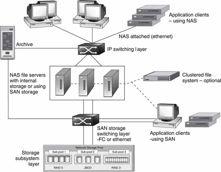
Consider an A/V edit cluster of N clients (craft editors and browsers), NAS or SAN attached. They may connect to one or more servers over a network. The servers in turn have access to storage. Clients may edit directly off the storage (direct to RT storage model) or use file transfer methods to load projects directly to the edit client.

Or consider an ingest and playout system. In this case the clients are ingest and/or playout nodes. Under control of a scheduler/automaton program or manual trigger, each of the clients will perform the record/playout operation on command. Some commercially available distributed video servers use the NAS method for client connectivity, and some use the SAN method. Most large-scale video servers from the major vendors are based on either of these two methods. See, for example, server products and systems from Avid, EVS, GVG/Thomson, Harris, Quantel, Omneon, SeaChange, Sony, and others. Small, standalone servers are often self-contained with no SAN or NAS storage connectivity, although they usually have a LAN port for file transfer support.

Clients may be A/V processors that are programmed to do effects, coding, or conversions of all kinds. One commercial example of this is the FlipFactory file conversion gateway from TeleStream.

Incidentally, Media Asset Management (MAM), automation control, systems management, and A/V proxy servers are not shown in Figure 3A.1. These elements are not relevant to the discussion at hand. Nevertheless, these elements are vital to any real-world A/V system, and their contributions are discussed in other chapters. Also not shown are any traditional (non-IT-based) A/V links. These links may always be added as needed.

3A.0.1 The Client and IP Switching Layers

The first (top) layer is the application client. The client types are discussed in detail in Chapter 2. Each client can access the NAS file server over a network. Technically, a NAS-attached client accesses the storage layer via the file servers. In some cases, however, the server layer will also provide application services, such as file format conversion, encoding/decoding of the stored essence, caching, bandwidth regulation, and more.

The second layer is IP switching. This can be as simple as a $100 switch or a complex campuswide mesh of switches. The reliability can be minimal or extend all the way to a fault-resilient network with various strategies of failover. Although Ethernet is the most common link, other less common links exist but are not the subject of this discussion. It is possible to design and operate this layer with excellent QoS with support for RT client access to the servers. See Chapter 6 for more information on switching.

3A.0.2 The Server Layer

The third layer is the server subsystem. Servers may be located anywhere across the network. In general, they may be storage servers or application servers that execute application code. The simplest configuration is a single NAS file server attached to storage. Microsoft offers the Windows Storage Server; many vendors use this as the core file system for their NAS products. At the other end of the spectrum is cluster computing with a mesh of servers working together as one. Cluster computing strategies range from a few independent servers that are load balanced to hundreds that appear as one virtual server. Fault tolerance and scalability are paramount in a cluster.

Grid computing is another technique that is differentiated from cluster computing (see Appendix C). The key distinction between clusters and grids is mainly in the way resources are managed. In the case of clusters, the resource allocation is performed by a centralized resource manager, and all nodes work together cooperatively as a single unified resource. In the case of grids, each node has its own resource manager, and overall there is no single server view as with clustering.

The big five players in the enterprise hardware server market are listed in Table 3A.1. The revenue includes any loaded OS software if present. The worldwide server market was $54.4 billion in 2007.

Table 3A.1 Worldwide Server Market

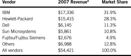
a Revenues are in millions. From IDC’s Worldwide Quarterly Server Tracker.

One unique incarnation of a server is called a blade. Compared to a standalone rack-mounted server, a blade is a server on a card that mounts into a multicard enclosure. The packing density, cost, and efficiency (shares’ power supplies, enclosure, and other elements) are outstanding. Blade servers accounted for 8 percent of all servers sold in 2007.

3A.0.3 The Storage Switching Layer

Layer four (Figure 3A.1) is the storage switching layer. In the simplest of cases, a server connects to a single storage array with barely a hint of switching or none at all. At the other end of the scale, the storage switching layer is a complex Fibre¹ Channel switching fabric (SAN) with failover mechanisms built in. More recently, some storage arrays support native Ethernet SAN connectivity based on iSCSI (SCSI protocol over TCP/IP). Fibre Channel has owned this space since 1998 so the migration to new methods will take some time. Note, too, that SAN clients connect directly to storage over Fibre Channel bypassing the server layer. A SAN-connected client (2 Gbps FC link, for example) has access to ~1,600 Mbps of storage bandwidth. Until recently, this type of performance has been available only using Fibre Channel.

Ethernet has won the war of enterprise connectivity and is pushing Fibre Channel lower in the value chain, although the two will coexist for many years to come. The trends to Ethernet/IP are very interesting, but legacy Fibre Channel SANs will not be replaced overnight. It is possible to build all five layers of Figure 3A.1 with only Ethernet/IP connectivity. During this transition, companies such as Brocade, Cisco, and HP provide gateways that link IP and Fibre Channel to create hybrid SANs. As a result, the modern SAN is composed of pure Fibre Channel at one end of the scale, a hybrid of IP and FC in the middle, and iSCSI at the all-Ethernet end of the spectrum. Replacing FC with Ethernet/IP has many implications, which are discussed in this chapter.

3A.0.4 The Storage Layer

Layer five, at the bottom, is the user storage layer. Of course, the storage system could be represented as tiered but is not here for simplicity. A tiered taxonomy is covered in Section 3A.7.1, “Data Flows Across Tiered Storage.” Storage systems range from a simple external USB2-connected array up to many Petabytes of Fibre Channel (or Ethernet)-connected arrays. At the high end, the arrays are complex systems of many drives (hundreds) with RAID protection and mirrored components to provide for the ultimate in reliability. For an example, of the ultra high end, see the TagmaStore from Hitachi Data Systems. There are various clever architectures from different vendors, all claiming some unique advantage in performance (access bandwidth + storage capacity + low access latency), reliability or packing density or usability (connectivity + management + backup + support) or price, or some combination of all of these. Storage is big business.

IDC (www.idc.com) reports the 2007 worldwide disc storage systems² factory revenue was approximately $26.3 billion (see Table 3A.2).

Table 3A.2 Worldwide Disc Storage Systems Factory Revenue

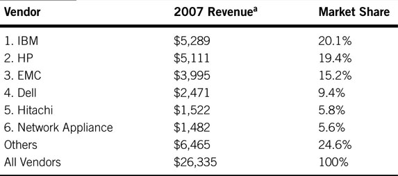
a From IDC, March 6, 2008. Revenues are in millions.

The storage subsystem shown in Figure 3A.1 is a mix of various types, ranging from RAM-based to disc-based RAID systems of various flavors.

If managed properly, a distributed storage system may appear as one array. When the methods of storage virtualization and/or clustered file systems (discussed next) are used, just about any mix of storage technologies may be combined into a homogeneous whole. While it is true that the storage system may be built from optical, holographic, or tape media, these are considered as archive or backup formats due to their slow access times.

3A.0.5 Long-Term Archive

The last piece of the puzzle in Figure 3A.1 is the long-term archive. This component may connect into layer two (NAS attach), layer four (SAN attach), or be accessed via FTP depending on the design of the overall system. Archives are normally based on long-term storage with removable tape or optical media. Most commercial archives have access times considerably slower than HDD arrays but offer much greater storage density. For most A/V applications, it is possible to find a content balance among online storage (HDD-based), nearline, and offline storage. For more on this topic, see Section 3A.7, “Hierarchical and Archival Storage,” later in this chapter.

3A.0.6 Storage Software

End users will continue to invest strongly in various forms of storage software. IDC forecasts the worldwide storage software market to pass the $17 billion mark by 2012, representing a 9.6 percent compound annual growth rate from 2007 through 2012. Storage systems are a strategic purchase for the media enterprise, so buy smart and insist on the performance, scale, and reliability that meets your A/V business needs.

3A.1 STORAGE VIRTUALIZATION AND FILE SYSTEM METHODS

With so many different devices connecting to the same storage system in Figure 3A.1, who is the traffic cop that regulates access? How does any one server or SAN client manage its storage pool? Who assigns access rights? What prevents a client from writing over the data space of another client? Who owns the directory tree? Well, there are two general ways to solve these sticky problems: storage virtualization and use of a clustered file system. Storage virtualization is considered first.

3A.1.1 Storage Virtualization (SV)

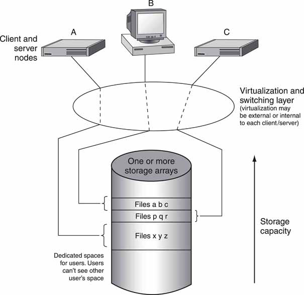
Storage virtualization partitions the entire array or collection of arrays into blocks that are individually assigned to select servers or SAN clients. This method insulates the requesting devices from the physical storage by providing a layer of indirection (filtering, mapping, aliasing) between the request for stored data and the physical address of that data. There are various ways to accomplish storage virtualization. In effect, the available storage is carved up into virtual pools that act as independent storage arrays. There is no common view of all storage from the client’s perspective but only the portions they are allowed to see.

For example, in Figure 3A.2 server A can see only files X, Y, and Z; client B can access only files A, B, and C; and server C has access to files P, Q, and R. The respective files reside in sections of memory that are assigned to the attached clients and servers. There is no shared file system view; rather, memory is carved up and apportioned as needed. Dividing up the memory this way guarantees access rights; server A cannot mess with files that belong to server C and so on. However, attached devices cannot share files easily because they are walled off from each other. Sometimes this is an advantage, and other times it is not.

FIGURE3A.2 Example of storage virtualization: Sharing storage HW.

So why do it? Here are a few of the main reasons to use virtualization:³

• You can manage all storage with a centralized application: This reduces labor costs to manage heterogeneous storage systems.

• Users and applications have better access to storage: User access to storage is not limited by geography or the capacity of an isolated storage module.

• IT administrators can manage more storage: Gartner Group estimates that managers can increase the amount they can administer by at least a factor of six if storage is consolidated.

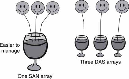
• You can lower physical costs of consolidated storage: Existing storage is used more efficiently because one pool (a SAN) is apportioned rather than managing DAS islands. In effect, it is more efficient to manage one pool with N straws drawing from it than N pools each with one straw (see Figure 3A.3).

FIGURE3A.3 A SAN is easier and less costly to manage than islands of DAS.

• You can scale with more reliability compared to DAS pools: Scale by adding arrays and then map their access as needed to multiple requesters.

• You can allocate capacity on demand.

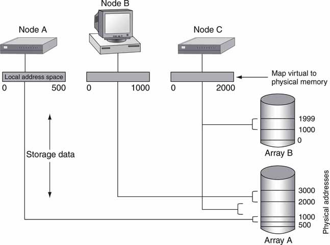
Virtualization is accomplished in several ways. The most popular is to map each node’s assigned storage space to a physical address. This is done using the mapping, aliasing, and filtering of requested addresses.

Figure 3A.4 shows a diagram of the concept. Node A has a storage address range from 0 to 500, which maps onto array A’s physical address 500 to 1,000. Node C has an address range from 0 to 2,000, which maps into two different arrays, each contributing a 1,000 and 1,001 address, respectively. Mapping is implemented in various ways, and logical unit number (LUN) masking is a popular choice. If done in the storage array controller, then it does the mapping based on the identity of the requesting node. Some vendors support the virtualization operation at the node level, switch, or storage array level, so the virtualization layer in Figure 3A.2 is a logical view, not a physical one.

FIGURE3A.4 Virtualization using address mapping.

The debate about where to locate the virtualization logic is an interesting one. The ANSI/INCITS group has released the fabric application interface standard (FAIS). This standardized API facilitates LUN masking, storage pooling, mirroring, and other advanced functions at the fabric switch level. As a result, FAIS enables advanced storage services, which adds value to the storage system and reduces the need for proprietary solutions.

The main public companies that support storage virtualization are the names in Table 3A.2, plus Brocade Communications Systems, Cisco Systems, and Symantec. There are many other smaller vendors offering hardware and software virtualization solutions.

3A.1.2 Clustered File System (CFS)

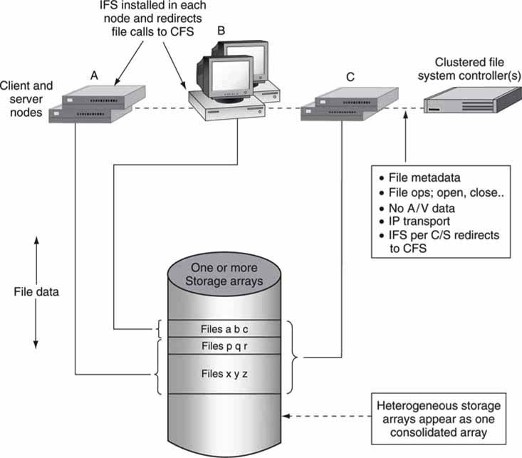
A second method for managing a storage pool is to provide every attached node (SAN clients and NAS servers) with a single, universal view of file storage. A clustered file system allows multiple attached devices to have read and write access via a single file system for all available storage. A CFS is also called a shared disc file system. However, this name is vague and somewhat misleading. With storage virtualization, only the physical storage is shared. With a CFS, however, storage and files are shared. File sharing is complex because clients/servers may R/W to any file (with permissions), thereby creating potential for multiple users to write over the same portion of data. So file-locking mechanisms are needed to ensure that files are reliably opened, modified, and closed. A full-featured, fault-tolerant CFS is a thing of beauty. Incidentally, no actual user data pass through the CFS controller; only file system metadata are managed.

In Figure 3A.5, the CFS is made available to all nodes. In the figure, it is not important how the nodes connect to storage, only that they do and all see a shared file system. In reality, each node has an installable file system (IFS) software component for redirecting all user application file calls to the remote CFS controller instead of the local file system. In Figure 3A.5, node B may access only files a, b, and c, whereas node C has access to all the files. This is markedly different from virtualization. With a CFS, any node has potential access to any file in storage given the preassigned access rights. There are no inherent walls as with virtualization; all storage is accessible from any node in principle.

FIGURE3A.5 Example of using a CFS: Sharing storage HW and files.

There are three main methods for a node to access a file system:

• Node uses only its internal file system. For example, a Windows server or client is based on Microsoft’s NTFS file system. This file system manages any direct attached storage (DAS or SAN based).

• Node connects to remote server (NAS attach) and sees that server’s FS (as in \Company_Serveryour_files format).

• Node has an installable file system software component to access an external CFS view of the storage. Each node can be part of a SAN or NAS. A node (or user of the node) selects the CFS view of the file system as it would select the CD-ROM drive or external file server (as in X: drive). The nodal platforms may be of any type (Linux, Windows, Mac, etc.), and a corresponding IFS is needed for each platform.

There is little magic in implementing the first two choices; they are commonly used. However, implementing a CFS is non-trivial. Why? Some of the common features are

• Negotiation of all R/W access to a heterogeneous pool of storage from a heterogeneous pool (Windows, Linux, Mac) of requesting nodes. Not all CFS implementations support all node types.

• Simultaneous users (hundreds or more) accessing up to millions of files.

• Data striping across storage arrays to increase access bandwidth.

• Data block locking, file locking, and directory locking.

• Bandwidth control to support QoS demands.

• Fault-tolerant operation using dual auto failover CFS metadata controllers. It may also implement a journaled FS (JFS) for supporting CFS failure with graceful recovery by performing a rollback to some stable FS state.

• Access control settings per user/group/campus.

The CFS must be a responsible citizen; it is a single point of file metadata for all member nodes. If it faults in some way, everyone is unhappy.

The CFS is a masterful administrator. It manages all the metadata that define a typical hierarchical FS: the storage access rights and permissions per user/group, address maps that associate physical user memory with directory/file names, and tools to create/read/write/delete files. Each node has a lowbandwidth TCP/IP (or even UDP) connection to the CFS, and over this channel all CFS requests/responses are made. The CFS must potentially support hundreds of simultaneous requests across the entire FS spectrum of operations. Indeed, creating and testing a CFS is a massive undertaking.

One welcome addition to the CFS world is NFS V4.1, the so-called Parallel NFS (pNFS). NFS is discussed in Chapter 3B. Basically, NFS enables a client to access single file servers across a network. pNFS enables a CFS with a global name space for all clustered file servers. Detailed coverage of this is beyond the scope of this book. However, pNFS is the first standardized approach to implementing a CFS and may gain traction as the preferred method over the next few years.

3A.1.3 Volume Management

Whether a system is configured for virtualization or a CFS, the concept of volume management is important. Many practical systems combine a pool of disc arrays into one or more volumes for user access. By hiding individual arrays and mapping them into volumes, you can more easily allocate array storage to individual users or groups. Figure 3A.6 illustrates a small system with four arrays. Array set A has three arrays, each with individual drives. The A/V files are striped across all three arrays. Striping provides for improved non-blocking access to files. Striping is discussed later in this chapter. Array set B is only one array. All four are virtually combined to be one 5TB volume V. Users do not know if their files are stored on arrays A or B and should not care in most cases.

FIGURE3A.6 Example of volume organization.

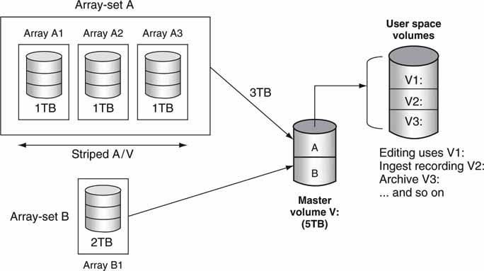
In some systems, volume V: can be further divided into user or group space. When a volume manager application is used, virtual volumes V1, V2, and V3 may be created and assigned as needed to the user community. The amount of assigned storage may be changed as needed for business processes. In advanced systems, user utilization and department billing are included. Volume management conceals the details of array configurations and provides simple volumes (V1:, V2:, V3:, etc.) for user access. For a simple example of a volume manager under Windows XP, access Control Panel, Admin Tools, Computer Management, and Storage.

3A.1.4 Distributed File System (DFS)

A distributed file system is differentiated from a CFS in how the FS is implemented. Both attempt to create a single file system image for all storage, but they do so in different ways. With a CFS, file metadata reside on a separate and dedicated FS controller (or more than one for fault tolerance). With a DFS, the FS is distributed among the nodes (servers normally) such that the FS function spans servers and is a part of each server node. Think of a DFS as a way to repackage a CFS by folding its functionality into the servers that access storage. Since a DFS spans, say N servers, they must all cooperate together to create the single FS image. It is easy to imagine that this is complex in terms of guaranteeing reliability, stability, and scalability. DFS success stories are rare, but the Andrew File System (AFS) is probably the most successful. It was developed at Carnegie Mellon University and is now available through open source as OpenAFS (www.openafs.org). AFS is supported by Linux as well.

Unfortunately, the term DFS is a bit overloaded. Indeed, even Microsoft offers a form of distributed file system, but it is not a DFS in the true sense. To make matters worse, many authors refer to a DFS as a CFS and vice versa because the two are so intimately related. However, Microsoft’s use of DFS is limited.

With Microsoft DFS,⁴ users no longer need to know the actual physical location of files in order to access them. For example, if marketing places files on multiple servers in a domain, DFS makes it appear as though all the marketing files are on a single server. This ability eliminates the need for users to go to multiple locations on the network to find the information they need. DFS also provides many other benefits, including fault tolerance and load-sharing capabilities, making it ideal for all types of organizations. As a result, DFS locates the actual files across a domain of servers and consolidates their appearance for easy browsing. The actual files remain on desperate servers and storage systems, but the view of these appears as consolidated to a user searching for files. Microsoft uses DFS in this limited way. It is not the same as a true CFS or its derivatives.

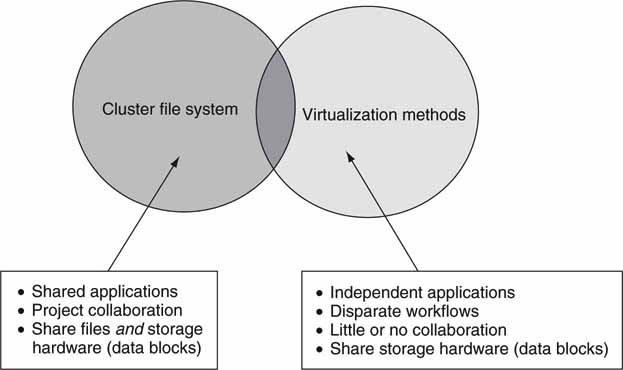
3A.1.5 Virtualization or CFS: How to Choose

So when would a facility use virtualization, and when would a CFS (or true DFS) be more appropriate? Figure 3A.7 shows that the selection of one versus the other is based on how users operate. With A/V applications, because users tend to share files, work in collaboration, and use the same types of tools, a CFS is appropriate. In a business setting (running SAP, ERP, CRM), users rarely collaborate between applications, so virtualization suits the usage patterns. In fact, both are used in organizations worldwide.

FIGURE3A.7 Individual benefits for CFS and virtualization.

In the technical and general business computing arena, several CFS vendors offer general-purpose (COTS) products:

• SGI’s CXFS (Clustered eXtended File System) 64-bit FS for Irix, Linux, and Windows access to storage (SAN) or servers (NAS). Supports up to 9 million terabytes of storage (9 Exabytes). This was designed to support A/V applications.

• IBM’s GPFS (General Parallel File System) for heterogeneous node access to a massive clustered server system. This CFS (actually a DFS) is not sold separately but only in conjunction with GPFS-clustered servers. IBM also offers the SANergy FS as a standalone product.

• Symantec’s (acquired Veritas) Storage Foundation CFS. This is used in general enterprise applications. The Veritas CFS delivers a cohesive solution that provides direct access to shared disks and files from all heterogeneous nodes in the cluster.

• Quantum’s StorNext FS for heterogeneous node access to storage.

• Apple’s 64-bit Xsan CFS.

• Sun’s open source Lustre FS. In testing on production supercomputing clusters with 1,000 clients, Lustre achieves an aggregate parallel I/O throughput of 11.1 GBps, utilizing in excess of 90 percent of the available raw I/O bandwidth. It is Linux based.

• Red Hat’s 64-bit Global File System (GFS) for Linux server clusters.

• Sanbolic’s Melio FS for heterogeneous node access to storage.

In addition to general-purpose CFS solutions, some captive CFS solutions are bundled with A/V SAN/NAS systems. These CFS products are included as a captive part of a vendor’s overall storage solution. In some cases the CFS is buried in the infrastructure and is not called out as a CFS, but it is. Most of the systems support NLE, video server I/O, and other nodal functions for news production, transmission, and general edit applications. Basically, if an A/V workflow requires file sharing among collaborators, then a CFS is an enabler. Following are some of the leading A/V systems that include a bundled CFS:

• Avid’s Unity ISIS storage platform for general editing, postproduction, and news production applications.

• Harris’s NEXIO advanced media platform (AMP).

• Omneon’s MediaGrid System with the EFS (Extended File System, a CFS).

• Quantel uses the Quantum StorNext CFS alongside its sQServer storage system. This is a COTS CFS integrated into an A/V environment.

• SeaChange Broadcast MediaCluster play-to-air video server with a customembedded CFS (actually a DFS) configured to work with each of the nodes in the cluster.

• Thomson/GVG K2 client/server with support for Windows-based transmission servers and news production nodes. This system uses the StorNext CFS from Quantum.

For the most part, these A/V vendors chose to build their own CFS and not use a COTS version. Why? There are several reasons. One is for total control in mission-critical environments. Another is based on a make-versus-buy analysis. Still another is performance related to reliability, failover speed (not all COTS versions are optimized for A/V applications), and integration with embedded client operating systems (non-Microsoft). Time will tell if the COTS versions will beat out the custom versions in the market. The COTS versions have massive engineering behind them and are feature rich. The A/V-specialized ones are niche products and may well get sidelined as the industry matures. Some of the COTS versions are A/V friendly, and this trend will most likely continue.

3A.2 CLIENT TRANSACTION TYPES AND STORAGE PERFORMANCE

Client applications conduct exchanges with servers and storage using a wide range of transaction types. Figure 3A.8 shows three of the most typical:

FIGURE3A.8 Storage transaction types.

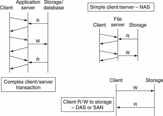
• Complex transaction. An example is to obtain the rights to edit a valuable piece of content. This may require exchanging user name, password, condition information, and purpose and also granting a use token. Note that the storage may be accessed several times during the transaction. A database (SQL Server, Oracle, MySQL, etc.) may be involved with this type of transaction.

• Simple transaction. An example is a NAS-attached client asking the server layer to read a block of video MPEG data from the storage array.

• Direct R/W transaction. An example is a direct R/W to storage using a DAS or SAN connection.

For each of these transactions, the storage system (HDD based for this analysis) is accessed, and its efficiency of performance depends on the access patterns. Four main aspects contribute to the overall performance of a storage system.

1. R/W patterns: Size of R/W block and random or sequential access to the HDD surface

2. Mix of reads versus writes from 100 percent read (0 percent write) to 100 percent write (0 percent read)

3. Utilization of the array from 0 to 100 percent usage

4. Capacity remaining from 0 to 100 percent

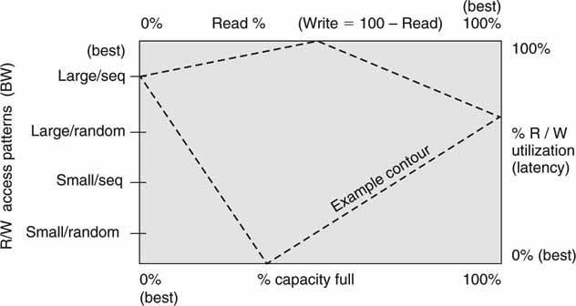
Each of these factors impacts various performance metrics. Figure 3A.9 shows a “billiard table” diagram with each side being one of the four factors just described. It is assumed that the array is not laboring under any failure modes (RAID data recovery in use). The purpose of the diagram is to encapsulate all four of the metrics into one visual imprint. Starting at the bottom left and moving clockwise around the outside, the left axis is a measure of user data access patterns (strong influencer of access bandwidth), the top is a measure of the mix of R/W transactions (influencer of access bandwidth), the right axis is the total throughput utilization (measure of latency), and the bottom axis is a measure of the remaining capacity of the array. For each of the four axes, moving clockwise is an improving metric. For example, the top of the right axis indicates 100 percent utilization of the array. For this case, the R/W requests form a deep queue, and therefore transaction latency is inevitable due to the heavy loading. However, the lower portion of the right axis is 0 percent utilization, so the occasional R/W request gets immediate response because there are no other requests to compete for storage resources. These four elements are developed in the following sections.

FIGURE3A.9 Storage system performance billiard table diagram.

3A.1.2 Optimizing Storage Array Data Throughput

Considering item 1 from the previous list, the two most important metrics that influence individual disc performance are block size and data seek method:

• Large R/W blocks (0.5 to 2 MB block), medium R/W blocks, or small R/W blocks (4 to 64 KB blocks).

• Random or sequential R/W data access:

Random: The next R/W may be at any physical address on the disc, causing the HDD head to seek to a new track.

Sequential: The next R/W address follows in order so that the R/W head of the disc does not have to seek a new track.

These factors are not relevant if the storage system is RAM based because RAM has no concept of rotating surfaces or R/W head movement. When you are using a HDD-based array, however, the seek time and rotational latency are very important. These are illustrated in Figure 3A.10. Seek time is the time required for a disc drive’s read/write head to move to a specific track on the disc platter. Seek time does not include latency nor the time it takes for the controller to send signals to the read/write head. Rotational latency is the delay between when the controller starts looking for a specific block of data on a track (under the head) and when that block rotates around to where it can be read by the read/write head. On average, it is half the time needed for a full rotation (which depends on the rotational speed, or rpm, of the disc). It is because of the seek time and rotational latency that the block size (large/small) and random/sequential access methods have such a big impact on drive R/W performance. As we shall see, the rpm of the platter (spans 7.5 to 15 K usually) is not a key factor in the average data throughput for large A/V data blocks. First, here is an illustration to help you better appreciate these issues.

FIGURE3A.10 Key access metrics for HDD performance.

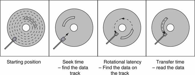
Let us say that you plan to go to Maui, Hawaii, for vacation. The airplane trip is analogous to the seek and latency times before you arrive. Once you arrive on Maui, you likely want to stay as long as possible. The longer you stay, the less bearing the initial air travel delay has on your overall journey. If it takes 5 hr to reach the island and you stay 2 weeks, then the one-way travel time is only 1.5 percent of your total vacation time. However, if you stay only for 5 hr and then hop on the red eye to return home, the one-way travel time was a huge part of the overall journey (50 percent). What a waste! This is the same as when doing a R/W transaction to a HDD. The bigger the data block, the more time is spent reading/writing compared to the travel time to get there.

As a result, the average R/W bandwidth is strongly related to block size; bigger blocks yield higher data rates on average.

What about random versus sequential access? When planning your tour of Maui’s best beaches, you could randomly visit five different beaches (Wailea, Hamoa, Kapalua, etc.) or plan to visit them by the most direct route, thereby saving travel time. This is the same as when doing a R/W access to a disc. If the R/W head does not seek to a new track (a sequential access) for each R/W transaction, then the overall throughput is increased compared to random R/W access. It is not always easy to place data sequentially (due to disc data layout strategies controlled by the OS), but A/V data lend themselves to this type of placement due to their large size and typical sequential access for a read. So let us celebrate long vacations with plenty of beach time.

These factors may be logically grouped into four specific access patterns:

1. Large blocks/sequential access (best A/V access rates)

2. Large blocks/random access

3. Small blocks/sequential access

4. Small blocks/random access (worst A/V access rates)

As per the reasoning thus far, the access bandwidth progressively improves from the worst case (bottom) item to the best case (top) item. It is arguable if items 2 and 3 are always positioned this way. For some cases they may in fact be reversed. There is a considerable performance gain between the top and bottom items. Figure 3A.11 shows the actual measured access bandwidth versus the block size for random R/W transactions.

FIGURE3A.11 Array performance versus block size.

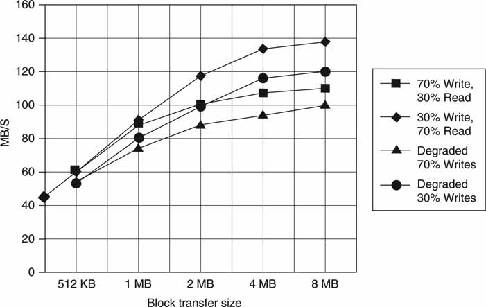
The test configuration is four data drives plus one parity drive in two RAID 3 sets. So in all, there are eight data drives and two parity drives. RAID is fully explained in Chapter 5, but what you need to know now is that it is a reliability mechanism to recover all the data from one (or more) faulty drive. All user data are striped across all eight data drives (RAID 0), so an 8 MB user block is split into eight 1 MB blocks—one per data disc. In Figure 3A.11, the aggregate R/W bandwidth for the multidrive array is 140 MBps, with a mix of 70 percent reads and 30 percent writes and a block size of 8 MB. The same R/W mix reaches only 60 MBps, with a block size of 512 KB and much less for a 16 KB block that is common in many non-A/V transaction applications.

Notice that the mix of reads versus writes has a profound effect on the array throughput. The top axis in Figure 3A.9 is a measure of the R/W mix. For a 30 percent read and 70 percent write mix, the bandwidth is about 110 MBps. Why is this? In a RAIDed configuration, a write has a penalty because the parity disc needs updating for every write to the four data drives. If user data are not striped across all data drives but are written to only one, then the write penalty is much worse. The reasons for this are developed in Chapter 5. A read does not need to access the parity drive unless there is a faulty data drive that needs restoration. Some vendors’ solutions activate RAID when a drive is late in returning read data, as this improves latency performance. Figure 3A.11 also shows data access rates under a “degraded mode.” This is the case if one of the data drives is being rebuilt (RAID node) in the background during R/W transactions. Rebuilding a drive steals valuable bandwidth from user R/W activity.

The right axis of Figure 3A.9 is a measure of array utilization. As mentioned, the more array transactions per second, the longer the delay to complete a transaction. Because transaction delay is never good, many systems are designed to operate at less than ~80 percent utilization for a given latency.

Another contributor to storage command-response latency is a large R/W data block. This is especially true when an array or HDD has many requests in queue. Large R/W blocks require a longer time to execute, so a deep commandresponse queue can add significant delay if not well managed.

3A.2.2 Fragmentation, OS Caching, and Command Reordering

The image of the storage array data layout starts looking like Swiss cheese if the R/W and delete block sizes are small. The result is called fragmentation. There are two types of fragmentation: file fragmentation and free space fragmentation. File fragmentation refers to files that are not contiguous but rather are broken into scattered parts on the disc. Free space fragmentation refers to the empty space that is scattered about rather than being consolidated into one area of the disc. File fragmentation reduces read throughput, whereas free space fragmentation reduces write throughput. Interestingly, if data are formatted in large blocks, then the fragmentation is a nonissue. In fact, sequential A/V files and fragmented A/V (random access) files have about the same access performance if the R/W block size is large according to the reasoning that has been developed. As a result, in many A/V systems, there is no need to defrag the arrays. This is good news because the defrag process is slow and might cause marked array performance problems for systems that operate 24/7.

In practice, it is the A/V equipment vendor’s choice to fine-tune drive access and improve array throughput and latency. Many operating systems decide when (waiting adds latency for reads/writes) and with what block size (may be very small, 16 KB) an array is accessed. For maximum performance, some A/V-centric applications bypass the OS services for managing the disc array access and rely on custom caching and R/W access timing.

The ideal model is for all access to be sequential (or random), large block transactions. However, it is often difficult to guarantee this, as small block transactions (metadata, proxy files, edit projects, etc.) and large A/V transactions are mixed for most applications. A mix of small and large block accesses can reduce the overall data throughput by up to 50 percent. For this reason, some vendors offer two different storage arrays for large A/V systems: one for large block A/V data and one for standard small block transactions.

HDD sequential R/W access has improved performance compared to purely random access for small block access. All modern drives have an internal cache for R/W queuing. So when a drive has, say, 10 random read commands in queue, then it can choose to reorder the access to optimize the read rate. A random command sequence of reads (or writes) is turned into a nearly sequential (approximates it) access operation. While it is true that read data may be returned out of order, the performance can be noticeably improved over the pure random access case. For most A/V applications, out-of-order returned data are resequenced easily by the application or other element. The extra logic needed to accomplish reordering is well worth the effort for the gains in performance.

The next section outlines common benchmarks for measuring storage system performance. Much of the reasoning that was developed in the previous sections is related to benchmarking. Figure 3A.9 is a way to visualize the factors that contribute to a performance benchmark.

3A.2.3 Storage System Benchmarks

Comparing storage system (SAN, DAS) performance and metrics can be a daunting task. By analyzing vendor data sheets and comparing specs, a reviewer may find a true apples-to-apples assessment to be nearly unattainable. This was the case until the Storage Performance Council (www.storageperformance.org) published its SPC-1 benchmark metric. The SPC-1 metric is a composite value of real-world environmental characteristics made up of the following:

• Demanding total I/O throughput requirements

• Sensitive I/O response times

• Dynamic workload behaviors

• Storage capacity requirements

• Diverse user populations and needs

SPC-1 is designed to demonstrate the performance and price/performance of storage systems in a server environment. The SPC-1 value is a measurement of I/Os per second (IOPS) that is typified by OLTP, email, and other business operations using random data requests to the system. The metric was designed to measure virtually any type of storage system from a single disk attached to a server to a massive SAN storage system.

Two classes of environments are dependent on storage system performance. The first is systems based with many users or simultaneous execution threads saturating the I/O request processing potential of the storage system. This type is typical of transaction processing applications such as airline reservations or Internet commerce. This spec is documented by SPC-1 IOPS. The second environment is one in which wall-clock time must be minimized (application based) for best performance. One such application is a massive backup of an array of data. In this case the total time needed to do the operation is crucial, so a minimum latency per I/O is crucial. This spec is documented by SPC-1 least response time (LRT) and is measured in milliseconds.

Of course, a storage system’s performance is not the same as the performance of an individual HDD. It is good to review the basic performance metrics for a single HDD. As with an array, the key measures are access bandwidth, seek/latency, and capacity. A typical high-end HDD drive has the following specs:⁵

• 400 GB capacity (SCSI type) with a maximum sustained read transfer rate of 100 MBps. Maximum sustained rates are rarely achieved in the real world because they are measured on the outer tracks of the disc only. The inner track sustained data rate is about 70 percent of the maximum value. A sustained transfer requires a large file, continuously available without seeks or latency delays.

• Burst I/O rates >1 Gbps. This is the HDD internal buffer to/from the external bus transfer rate.

These are truly amazing specs and drive vendors keep pushing the speeds and capacity higher and higher. The usable, average transfer rates for large files may be 70 percent of the maximum value. Of course, for many A/V applications, system design demands specifying the worst case transfer rate, not the best or even average case. The HDD seek/latency spec is almost frozen in time (does not follow Moore’s law), which affects the number of transactions per second that a drive can support.

ACCESS DENSITY

Disk drive performance is improving at 10 percent annually despite storage density growing 50–60 percent annually. Raw disk drive performance is normally measured in total random I/Os per second and can surpass 100 I/Os per second.

Access density is the imbalance between storage density and performance. Access density is the ratio of performance, measured in I/Os per second, to the capacity of the drive, usually measured in gigabytes. Access density I/Os per second per gigabyte. For streaming video, I/Os per second is not always an important metric, because long I/Os are common.

3A.3 STORAGE SUBSYSTEMS

This section outlines several modern storage architectures. The following technologies are core to the modern AV/IT architecture. The following storage methods are discussed:

1. JBODs and RAID arrays

2. NAS servers

3. SAN storage

4. Object storage devices

In each case the technologies are examined in the light of A/V workflows. To fully appreciate storage requirements, check out the storage appetite for various video formats in Chapter 2. Fundamental to all storage subsystems are the actual storage devices. For our consideration, RAM, Flash, and HDD cover most cases, either alone or in combination. Optical is applied to some nearline and archive storage and is considered in Section 3A.7.3, “Archive Storage Choices.” See for a review of the pros and cons of Solid State Disc technology.

3A.3.1 HDD Capacity and Access Data Rate

Every HDD provides storage capacity and an I/O delivery rate. These factors are both important and often misunderstood. We tend to think of a HDD as being defined by its capacity, as in “I just bought a 750GB hard drive at Fry’s Electronics.” That may be true, but that same drive also has an I/O spec. So, it is just as valid to say, “I just bought a 200 Mbps drive at Fry’s.” Disc bit density has increased about 60 percent annually since 1992, but storage device performance (random I/Os per second) is improving at only 10 percent per year. See the Snapshot on Access Density.

Drive vendors are focused on capacity more than increasing the I/Os per second or raw R/W rates. Some applications need capacity (a PVR), whereas some need I/Os per second (a Web server with thousands of simultaneous clients). Here are some practical requirements for two applications:

• Centralized VOD server with the top 30 movies serving 1,000 individual viewers (cable TV premium service), each with PVR-like capabilities. Thirty 2-hr movies require only 135GB at 5 Mbps encode rate (one drive). The aggregate read access rate is 1,000 times 5 Mbps 5 Gbps. If a single HDD has a spec of 15 MBps, then it takes 42 drives (all movies replicated on all drives) to meet the read access rates. For this case it is wise to use RAM storage. For 10,000 viewers, things get messy, and clever combinations of RAM and HDD are sometimes needed and/or some restrictions on PVR capability.

• At the other end of the scale is the case of 100,000 hr of 0.25 Mbps proxy video. Any of the content may be viewed by 200 desktop clients at once. To store the proxy files requires 11.25 TB total. If each HDD has a capacity of 250 GB (at 15 MBps), then it requires 45 drives to store 11.25 TB. The read bandwidth needs can be met with one drive (6.25 MBps total for 200 viewing clients).

Figure 3A.12 illustrates the two-dimensional nature of capacity versus access data rate. Four quadrants represent four application spaces each with their unique needs. As may be seen, applications range from requiring low capacity and low rate to those needing both high capacity and high rate. Knowing what dimension, if not both, you may need to scale is vital for reduced upgrade headaches down the road. For each application the total HDD count needed depends on whether the storage capacity or access date rate is the driving factor.

FIGURE3A.12 Example HDD array capacity versus I/O rate needs per application.

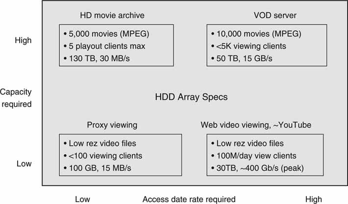
So it is obvious that storage capacity is not the only HDD spec of importance when doing an A/V system design. The examples prove that the HDD disparity between required capacity and delivery rates can reach a factor of 40 or more for some designs. The extreme YouTube example in the figure requires ~40 HDD to support data delivery compared to one HDD for pure storage capacity needs. There are lively debates in the VOD design community over the best way to store the content. Some vendors use only HDDs, others use RAM only, and some offer a hybrid of HDD/RAM to meet the demanding needs of capacity and bandwidth.

THE CASE OF THE MISSING 90GB

In computing, it is standard to use KB as representing 1024 B. Likewise, MB is 1024 KB, and GB is 1024 MB. This is thinking⁶ in a power of 2. So KB = 2¹⁰ bytes, MB = 2²⁰B, GB 2= ³⁰B, and TB = 2⁴⁰B. Disc drive manufacturers, however, use KB to represent 1,000B, MB = 10⁶, and so on. A 300 GB capacity HDD is exactly 300 × 10⁹ bytes, but when the drive is installed in most computer systems (Windows based, for example), its capacity is expressed using a K, M, or G based on 1,024 B. Just a tad confusing.

For example, a 1TB HDD would show an installed capacity of 0.91 TB (091 * 2⁴⁰, = ~10¹²) so a 1TB (1,000B reference) HDD is the same as 0.91TB (1,024B reference). There is about a 90 GB difference between the two methods. The “error” (—9 percent) is not trivial, but not an actual loss either. Do not confuse this with the difference between raw and formatted capacity—that is a true loss of useful capacity.

3A.3.2 Aggregate Array I/O Rates

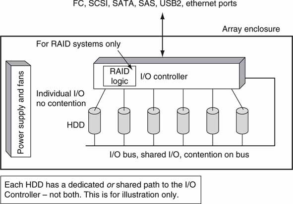
An array filled with, say, N identical drives will deliver N times the storage capacity of one drive, but the aggregate I/O rate will not always be N times the I/O rate of one drive. Why? Drive I/O rate depends on how the I/O controller manages drive access. Is there an individual link from each HDD to the controller, or are all HDDs connected together on a common bus or arbitrated loop? Both methods are shown in Figure 3A.13. In the first case the drives have individual access to the I/O controller, so there is no contention among drives. In the second, all drives will share I/O bus resources; hence, simultaneous HDD access is impossible. Aggregate access rates depend on several factors, and file striping is one of them.

FIGURE3A.13 A simple JBOD or RAID array.

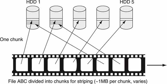
3A.3.2.1 File Striping and Array Performance

File striping increases access bandwidth by distributing the files across all drives in an array (or even across arrays). Figure 3A.14 shows one method of file striping to increase the aggregate access bandwidth. Because the file is divided among N drives, ideally, the file access rate is N times the case of the file being stored on one drive on average. Distributing a file across N drives allows more simultaneous clients to access the same file. One downside of this scheme is the vulnerability to file loss in the event of a HDD failure. If any one unprotected drive fails out of N, then the entire file is lost in practice. This increases the need to provide fault-resilient methods to store data (see Chapter 5). When several users need simultaneous retrieval of the same file, accessing the discs out of order reduces HDD queuing delays. The methods used to avoid queuing delays are varied and beyond the scope of our discussion, but they can be managed to achieve good performance. Also, if the HDD I/O bus burst rate is much faster than its R/W platter rate, then some of the contention will be reduced.

FIGURE3A.14 File striping example across five discs.

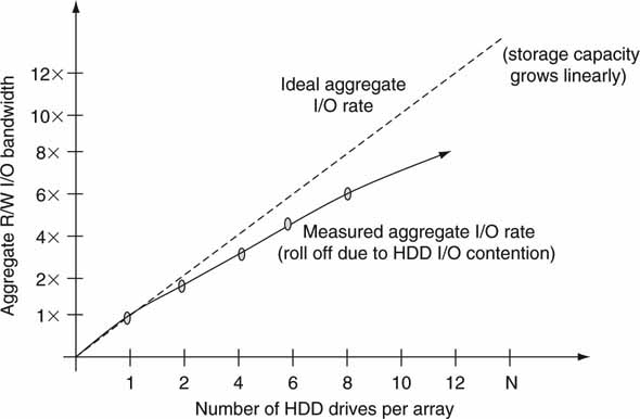
Generally, if there is HDD I/O contention (I/O bus connection in Figure 3A.13), an array offers an access rate profile, as shown in Figure 3A.15. Figure 3A.15 is derived from measured results and shows a 25 percent reduction (75 percent of ideal) in aggregate I/O when there are eight drives sharing a common I/O bus. This phenomenon is also seen when files are striped across multiple arrays each with N internal discs. Your mileage may vary, since the rate reduction is a result of contention mechanisms that will differ among storage subsystems.

FIGURE3A.15 Storage array aggregate I/O bandwidth versus number of drives.

Optimizing and managing capacity and access rate at the HDD or array level are not child’s play. Most A/V vendors tackle these issues in different ways. When evaluating a storage system, ask the right questions to fully comprehend what the real-world performance is.

The following summarizes the main points when adding capacity and/or I/O bandwidth to a system:

• Adding arrays or discs to an existing system adds storage capacity.

• However, the new capacity is made available to clients based on the configuration settings of SAN virtualization or a CFS if present.

• Adding arrays or discs to an existing system adds I/O capacity. However, the amount of R/W bandwidth available to clients depends on the presence of striping techniques and configuration of any SAN virtualization or CFS if present.

3A.3.3 General Storage Requirements

There are several factors to consider when selecting or defining a storage system.

• Usable capacity after accounting for redundancy (reliability) overhead.

• Usable R/W bandwidth considering the usage patterns: sequential, big block I/O, random or small block I/O. Remember, accessing small audio or proxy files (small block size usually) is markedly different from accessing high bit rate (large block rate usually) video files.

• Usable R/W bandwidth after accounting for RAID HDD rebuild methods.

• Reliability methods.

• Failover methods—done in A/V real time or not.

• Management methods—faults, warnings, alarms, configuration modes.

• A host of other features that may be significant depending on special needs.

When you are selecting a storage system, it is good policy to ask questions about these factors. There is no list that covers all user needs, so take the time and investigate to really understand the ins and outs of any system under investigation.

Many A/V facility owners/operators desire to use COTS storage (read cheaper) when configuring NLEs and video server nodes on shared storage. In general, however, these systems require A/V vendor-specified and tested storage systems (read expensive) to meet a demanding QoS. COTS storage vendors are happy to provide a generic product, but when it fails to meet the required QoS, they often will not make the needed upgrades. However, A/V vendors guarantee that their provided storage works well in demanding QoS environments. The bottom line is that COTS storage may work for some A/V workflows—if the shoe fits wear it—but A/V vendor-provided storage should always function as advertised. Next, let us examine the five basic storage subsystems found in various forms in most IT infrastructures: JBOD and RAID arrays, SAN, NAS, and object storage.

3A.4 JBOD AND RAID ARRAYS

There is nothing sophisticated about just a bunch of discs (JBOD), but you’ve got to love the name. It is the simplest form of a collection of disc drives in a single enclosure. Figure 3A.13 shows an example of a JBOD with either individual HDD links or a common I/O bus approach. It is really just an enclosure with power supplies, fans, drives, and an optional I/O controller board. The I/O controller may act as a gateway between the I/O ports (FC, SCSI, SATA, SAS, USB2, Ethernet ports) and the internal drive I/O. By definition, there are no RAID functions. Advanced array features such as iSCSI I/O using Ethernet are possible but more often are found on RAID arrays. Admittedly, there is no precise definition of a JBOD, but simplicity and low cost reign. Pure JBODs lack the drive reliability that is often demanded, so their use is confined to areas where reliability is not of prime importance.

When JBODs grow up, they become RAIDs. No, this type of RAID is not bug spray. A RAID—Redundant Arrays of Inexpensive (or Independent) Discs—describes a family of techniques for improving the reliability and performance of a JBOD array. A RAIDed array can allow one (or two in some cases) of N discs to fail without affecting the storage availability, although the R/W performance may degrade. This concept is now accepted as de rigueur, and many hard disc arrays offer RAID functionality. See Chapter 5 for a detailed discussion of RAID techniques and categories.

3A.5 NAS AND SAN STORAGE

Network attached storage (NAS) and storage area networking (SAN) are discussed in Chapter 3B—a chapter dedicated to these technologies. In a nutshell, both technologies are used to provide storage to network attached nodes. A NAS provides remote resources for both sharing storage and sharing files. A SAN, in its most native configuration, provides only shared storage resources. With the use of a CFS, discussed earlier, a SAN may be configured to share files among attached nodes. Clients attach to a NAS using Ethernet usually. Clients and servers attach to SAN storage using Fibre Channel and, more recently, Ethernet. General-purpose servers (including NAS servers) often use SAN storage. They both can offer excellent A/V performance and are the bedrock of many AV/IT systems.

3A.6 OBJECT STORAGE

A novel class of storage is object based. It differs from traditional file (NAS) or block-based (SAN) storage in several ways. Object storage devices (OSDs) store data not as files or hard-addressed blocks, but as objects. For example, an object could be a single database record or table—or the entire database itself. An object may contain a file or just a portion of a file. An OSD is a contentaddressable memory (CAM). If you provide it with an identifier (metadata fingerprint), it will return the content represented by the ID. The fingerprint is formed using a hashing algorithm for generating a unique 128 B (or similar) value that is used to identify and retrieve data.

Imagine that a 30 s video program has a fingerprint ID of value X and that this value uniquely represents it. If only one bit changes anywhere in the video, say due to a pixel change, the value of X changes. In practice, a requesting client asks for file ABC, which translates to a pointer of value X, and the OSD locates file ABC using this pointer. Depending on the implementation, clients may access the storage using CIFS/NFS (discussed in the next chapter) or via a custom API provided by the OSD storage vendor. OSDs are finding applications as near-line or secondary storage, so they will not be replacing traditional highperformance RT storage any time soon.

Objects are stored on OSDs that contain processors, RAID logic, network interfaces, and storage hardware. Each OSD manages the objects as it deems necessary. The OSD hides the “file” layout, addressing, partitioning, and caching from a requesting client. Objects may reside on one OSD or be partitioned across a network of OSDs. This abstraction is practical for some file types such as X-rays, images, videos, email archives, and a myriad of documents that are normally recovered whole. Partial access is also allowed. Using metadata to track and manage files adds flexibility in scalability, performance, location independence, authenticity, and reliability compared to traditional addressable storage. The value of the metadata fingerprint also maintains the integrity of the file against changes.

Linux server clusters are one means to implement OSD systems. Among the vendors in this space are Panasas (www.panasas.com) and Permabit (www.permabit.com). Other companies are attacking the market with standalone storage systems (not based on Linux clusters). For example, EMC’s Centera and HP’s Integrated Archive Platform are object-based stores. Network Appliance (www.netapp.com) offers NearStore Appliance (not object based). NearStore is going after the same market segments (near-line, secondary storage) as Centera but without using object storage.

Object storage is a new model and will find some niche applications over time. A/V data types are ideal candidates to be treated as objects. Sample systems that may use OSDs are a post house or film studio with thousands of hours of digital content. Each piece of material (or any derivatives) will have a unique fingerprint that may be used for asset tracking. Because OSD systems can scale to >100 TB with NSPOF reliability, they are also ideally suited for mission-critical near-line storage

The SNIA (www.snia.org) has defined XAM (eXtensible Access Method) as the preferred way to access object stores. XAM provides an API for importing/exporting files to an object store. Note that access to an object store does not use the ubiquitous NFS or CIFS protocols. So, the XAM API enables a standard method to achieve cross-vendor compatibility for store access. XAM also enables users to associate metadata for each stored object. Traditional file systems don’t register file-associated metadata. Knowing about the stored object (who, what, when info; IPR rights windows; legal aspects; and so on) is a huge value to a media organization. Expect to see XAM used by enterprise media companies.

3A.6.1 Deduplication

One special case of object storage is called deduplication, or single instance storage technology. This is a method for reducing storage by eliminating redundant data found across multiple files. Only one unique instance of the data object is retained in storage. Redundant data are replaced with a pointer to the unique data segment. For example, a typical email trail might contain many repeated textual segments. When you add new text to a received email and then send a reply, a new file is created that may contain 90 percent of the text from the previous email in the trail.

Squeezing out the repeated text (or other object) across many files can yield compression rates of 20× to 50× to in many business environments, according to the Enterprise Strategy Group (www.enterprisestrategygroup.com). Don’t expect any gain for single compressed A/V files; the air has already been expelled.

3A.7 HIERARCHICAL AND ARCHIVAL STORAGE

Installed digital storage is expected to grow 50–70 percent per year for the foreseeable future. (See Appendix D.) The economics of storing all this on RAM or even hard disc is untenable. As a result, IT has developed a hierarchy or pyramid of storage to balance the needs of users and owners of digital data. Each step in the hierarchy trades off access rates, capacity, and cost/GB. These three metrics are the key drivers behind the idea of tiered storage. Next, we consider a brief analysis of the trends in tiered storage.

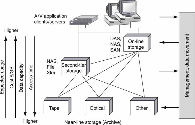
Figure 3A.16 presents a simple view of a three-tier storage system. The IDC classifies hierarchical storage into five tiers for normal business systems. For A/V, we will consolidate into three layers. Some ranks may not be present in all systems (no near-line, for example), but our analysis considers the fullfeatured case. At the top are the application clients and servers that demand fast data access times with unlimited access to stored data. Online SAN or NAS storage is typical with speedy access times (in the A/V real-time sense—mission critical) but with limited storage. Lower in the chain is second-tier storage. The trade-off here is giving up low access times for less expensive ($/GB) storage with more capacity. Second-tier storage may not guarantee RT access under all conditions. At the bottom is the archive layer and near-line storage. Here, excellent capacity and lower $/GB are the key metrics, with access times being very slow compared to HDD arrays. It is not uncommon for missioncritical storage to cost 10 more in a $/GB sense compared to slower offline (archive, many hour access time) storage.

FIGURE3A.16 The hierarchy of storage.

In addition to the economic needs of trading off access rates, capacity, and cost, there are several business uses of tiered storage:

• Long-term archive

• Daily server backup/restore

• Disaster recovery copies

• Snapshots creating a point-in-time copy of data for quick recovery

• Data mirrors for regional access or improved reliability

• Replication—like mirroring but writes are asynchronous

Most of these factors are discussed in Chapter 5.

3A.7.1 Data Flows Across Tiered Storage

The flow of data between the different storage elements is outlined in Figure 3A.17, the storage onion. Four sample flows are identified. Flow “A” is the common client to DAS/NAS/SAN storage connection. In most cases the client controls access to the online storage pools. In case “B,” data move between the archive and a second-tier store. The client layer is unaffected by the transfer of content when it occurs. However, some director (controller) moved the files, perhaps based on a JITFT schedule, for later use by a client/server or transfer across a WAN.

FIGURE3A.17 The storage onion—sample data movement paths.

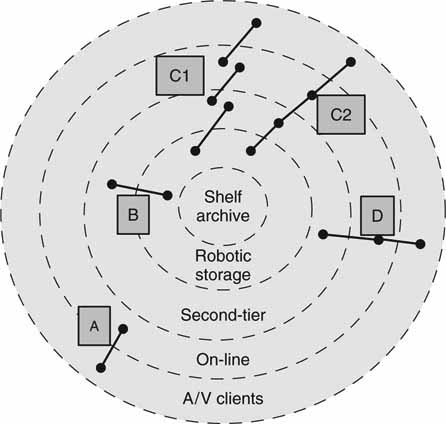
In flow “C,” data are moved from archive to client (or in the opposite direction) in either separately completed steps (C1) or as part of a continuous data flow (C2). In the first case, a director moves data between stores in steps as needed by schedules or other requests. There may be a wait period (minutes to days) between steps in the chain. In the second case (C2), a director moves data from the archive to second-tier to online in one continuous step for use by the A/V client. One example of this second case is a request for an ASAP A/V playback of some archived material. The playback file is located on the archive and moved to the second-tier store. As the second-tier store is being loaded, the target file is moved to the RT online store. As the online store is being loaded, playout of the file may commence. Sure, it may be more logical to move the file from the archive directly online, but let us use the C2 flow as an example only.

Now, the C2 flow is tricky, but it can be implemented with proper attention to data streaming rates. Compared to C1, C2 requires a high-performance QoS for each element in the chain and strict attention to the timing of the flow. From request to client playback start may take 15 s to several minutes depending on the archive type (optical or tape). The flow of data along the C2 path must be continuous and never “get behind” the playout consumption data rate; if so, the playout data will dry up. The data flow across all devices in the chain must, on average, meet RT playback (or record) goals. Frankly, the continuous C2 flow is an unlikely workflow in the real world. The stepped version C1 is practical and done everyday in workflows like those at Turner Entertainment’s Cartoon Network (see Chapter 10). Of course, C1 may require ~15 min (or less with fast transfers) to transfer a 5-min file along the path. It is more likely to see an archive to online continuous transfer (skip the second-tier stage) if there is pressure to play out ASAP. The bottom line is that both C1- and C2- like flows are practical in the real world.

The last flow is task “D.” This is a traditional two-stage file transfer from second-tier to online to playout. Typically, automation software schedules the transfers (JITFT mode) between near-line and online and initiates the playout at the client. D may be either of types D1 or D2, as with the C flow. If D is implemented, D1 is the more common flow.

Some AV/IT workflows use all of these methods (A–D) in harmony. However, not all A/V facilities have need for an archive, but some do. For example, Turner Entertainment uses a Sun StorageTek PowderHorn tape archive just to store its 6,000 cartoon library. Turner uses a true three-tier storage approach (C1) for the Cartoon Network and a two-tier approach (D1) for other networks.

The cost to manage data can be enormous, and it is one of the biggest issues in IT today. A/V workflows do not escape the management burden. Despite the nearly 70 percent increase in data annually, there is only a 30 percent increase in the ability to manage these data. So what are the best practices to manage data?

3A.7.2 Managing Storage

Over the years different strategies have emerged to manage storage. For many years hierarchical storage management (HSM) has been the mainstay for large enterprise data management. The most current thinking is centered on information life cycle management (ILM). ILM is the process of managing the placement and movement of data on storage devices as they are generated, replicated, distributed, protected, archived, and eventually retired. ILM seeks to understand the value of data and migrates them across storage systems for the most costeffective access strategy. A report from Horison Information Strategies [Horison] states that enterprises need to

Understand how data should be managed and where data should reside. In particular, the probability of reuse of data has historically been one of the most meaningful metrics for understanding optimal data placement. Understanding what happens to data throughout its lifetime is becoming an increasingly important aspect of effective data management.

The concepts behind ILM are useful for any A/V facility design, expansion, or rethinking of current storage strategy (see [Glass]).

Implementing an ILM strategy requires a combination of process and technology. Some process-oriented questions are as follows:

• What is the value of data as they age?

• Do data become more or less valuable?

• How long should we keep data?

• What storage policies can we apply to our data?

• What is the right balance of our data across the hierarchy to optimize ROI and user experience?

• Do we understand the different data types that drive our business?

Figure 3A.18 posits one possible scenario of data reuse as they age. Figure 3A.18 is general, and various data types exhibit different access signatures. Knowing that access rates decline over the life of data allows automation logic to migrate data to less costly storage. A/V data typically fall into a similar pattern.

FIGURE 3A.18 Data access rates decline with age of data.

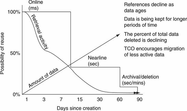
Source: Horison

Several companies specialize in managing the A/V data archiving process. EMC (AVALONidm), Front Porch Digital (DIVArchive), Masstech Group (MassStore), SGL (FlashNet Archive Manager), and SGT are among the few that cater to the special needs of the A/V industry. They provide software to manage the migration across the hierarchy and R/W from storage robotics. What makes managing storage special in A/V facilities? A few aspects are A/V data flows involving very big files (15 GB movies), partial file restore, appreciation for metadata, unusual A/V gear compared to enterprise devices, and time-critical delivery. Some traditional A/V equipment automation companies manage data movement between near-line and online storage as well.

Most large-scale facilities need both storage management and control automation software solutions to meet all their A/V data flow needs. As online and offline storage capacity increases and prices drop, fewer designs demand a full three-tier solution.

Many large broadcasters use tape archive systems. Sometimes the content is owned by the broadcasters (movies, dramas, for example), and they expect very long-term storage. Alternatively, the archive may cache materials for several months or years for reuse later. One example of programming reuse is at KQED in San Francisco, a PBS member station. This station stores up to 12,000 hr of PBS programming locally in a Quantum archive for reuse as needed. See Chapter 10 for a case study on KQED.

3A.7.3 Archive Storage Choices

Offline archive devices can be complex and usually involve some or all of the following:

1. Tape and/or optical removable media

2. Drives to control and R/W the media

3. Robotics to insert/remove media from drives

4. Housing for controllers, media, drives, and robotics

There has been a debate about what is a true archive media format. Some vendors tout 7–15 years media life as an archive format, whereas another will say that true archive needs a 35 + year media life. Although a worthwhile discussion, let us bypass this argument and treat any data tape or optical media as an archive format.

Archive devices are divided into at least three different camps: tape (helical and linear heads), optical disc, and holographic. In the mainstream, tape is the most popular, followed by optical. Some vendors manufacture all the components in the value chain, whereas others offer only pieces. For example:

• Sony manufactures media, robotics, and enclosure for the PetaSite tape storage system. The PetaSite supports up to 1.2 Petabytes (10¹⁵ bytes is one Petabyte). One Petabyte of capacity can store ~100,000 movies at a 10 Mbps compressed rate.

• Spectra Logic manufactures the T-Series tape robotic system. It supports SAIT and LTO drives and media. This system scales from 50 to 680 tapes and 24 drives.

• Imation manufactures tape media, including format support for DLT, Ultrium (LTO), and SAIT media.

3A.7.3.1 Magnetic Tape Systems

The magnetic tape industry produces more than 10 different recording formats with nearly 15 automated tape robotic suppliers. Single cartridge capacity is expected to approach ~3 terabytes in ~2011 based on planned improvements in recording density. The automated tape market is expected to grow as archive and disaster recovery requirements increase due to all things going digital (Moore 2002).

Out of the total, there are four top players in high-end archival tape formats. Sony offers AIT/SAIT (Super Advanced Intelligent Tape). A consortium of several vendors created the LTO (Linear Tape Open) format branded as Ultrium. Sun’s StorageTek brand offers the 9 × 40 tape format family. Quantum offered the DLT/SDLT (Super Digital Linear Tape) format for many years but discontinued it in 2007 in favor of LTO.

The current format leader is the LTO-4 with 800 GB native capacity at 120 MBps R/W rates. Figure 3A.19 shows the roadmap for the LTO format, the likely end winner in the format wars.

FIGURE 3A.19 LTO Roadmap (LTO-5,6 estimated dates).

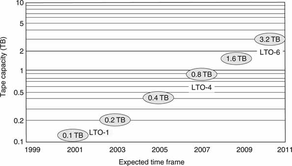
Also, both Sun and IBM have created “LTO-like” drives with native capacity at 1TB in 2009. LTO uses a “linear serpentine” recording format that stripes the data back and forth across the tape rather than the helical head scan format that was common for many years. For the economy minded, Sony and HP have co-developed a version of Digital Audio Tape (DAT) that has a native capacity of 320 GB at 86 GB/hour rates.

SMPTE is developing a tape layout format called the Archive Exchange Format (AXF). Any data tape that vendor A writes to using AXF can be read by vendor B. Before AXF, end users were locked into one vendor for all archive management needs. This is an untenable situation given the value of the media on the tape and possibility of the vendor defaulting.

In closing, a complete analysis of storage system performance involves metrics beyond tape formats. Other metrics include storage capacity per square foot and cubic foot of enclosure space, aggregate R/W throughput, tape retrieval time, search time, overall capacity, cost per TB (or per MBps), and line power needed per TB. Depending on your workflow, space, and power needs, these metrics have varying value.

3A.7.3.2 Optical Systems

Optical systems have always lagged behind magnetic tape in capacity and data rate, but recent products show promise for low-cost archives. Optical discs come in several flavors, including

• DVD with a single-sided, dual-layer capacity of 8.5 GB (single layer is 4.7 GB).

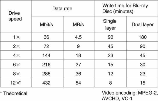
• Blu-ray disc is the crowned DVD successor format for HD. Secondarily, the format serves as pure data storage. See Figure 3A.20. At least one vendor supports 8 burner speeds in 2009. Plasmon, HP, and others offer Ultra Density Optical (UDO) with up to 60GB density per disc.

FIGURE 3A.20 Key parameters of the Blu-ray disc format.

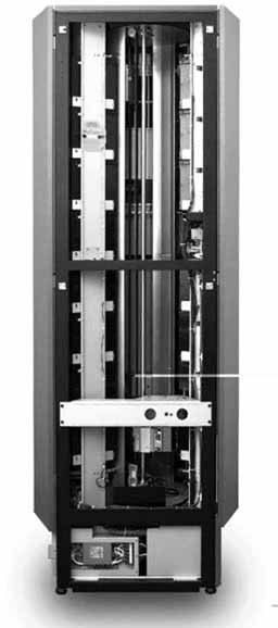
Optical R/W rates are much less than for tape, but their access times are better by a factor of 50 or more. Also, the robotics for managing optical discs tends to be less expensive than tape robotics because the disc is very light and easy to maneuver. The optical-based archive is finding applications in A/V facilities worldwide. One example of an optical storage system is the TeraCart from Asaca Corp. It supports SAN and NAS connectivity and Blu-ray discs with an enclosure capacity of 9.8 TB in only 4 square feet of footprint. More than 2,000 hr of 10 Mbps programming can be stored in one relatively small unit. Up to eight libraries may be connected to act as one unit. Figure 3A.21 shows this unit, the AM420PD.

FIGURE 3A.21 Asaca TeraCart using ProDATA storage (9.8 TB).

3A.7.3.3 Other Archive Devices

This section reviews some new and promising methods to archive data. One that is starting to gain momentum is Massive Array of Inactive Discs (MAID). The concept behind MAID is HDD-based storage designed specifically for write once, read occasionally (WORO) applications, where the focus is on infrequent access rather than I/Os per second. Applications that only occasionally access data permit the majority of discs not to spin, thereby conserving power, improving reliability, and simplifying data access. A typical MAID architecture may have only 1 percent of data spinning at any one time. Data access is measured in milliseconds to seconds—the time it takes to spin up a drive. MAID will have application in broadcast facilities where archived data are accessed only occasionally—say, to load a day’s playlist. MAID is not used for long-term, deep archive.

Holographic storage has been a promising technology for years. Until recently, it seemed as though it would languish forever in the laboratory. However, InPhase Technologies (www.inphase-technologies.com) has recently developed a WORM product (Tapestry) with 300 GB of capacity at 20 MBps transfer rates with a roadmap to 1.6 TB/120 MBps on a single platter. Several of the value propositions for holographic storage are leaders in density per cubic foot (32TB/cubic foot), 50-year media life (magnetic tape is 8 to 20 years), and reading rates faster than Blu-ray (factor of ~2× in 2008). Not to be ignored is the cost of the media itself. Holographic discs promise to be the low-cost leader compared to tape or other optical storage systems. Of course, holographic storage is immature and needs industry experience before it takes any appreciable market share from tape or optical.

A promising approach to achieve storage is the Pergamum project developed at the University of Santa Cruz (Pergamum). It uses a distributed network of intelligent, MAID-based, disk-based storage appliances (bricks) that store data reliably and energy-efficiently (~2.5 W per TB stored). Pergamum uses both intra-disk and inter-disk redundancy to guard against data loss. Each brick is Ethernet connected to create a unit that allows for obsolescence replacement with other commodity bricks.

3A.8 IT’S A WRAP: SOME FINAL WORDS

Storage technology is at the heart of all AV/IT systems. A good understanding of these concepts will help you better evaluate vendors’ products. Plus, you will be able to decipher vendor speak when it comes to their storage offerings and connectivity. Expect to see the “pocket server” in a few years as HDD density continues to head into the stratosphere. Storing 500 hr of content on one drive is not far off, and small A/V media clients scattered throughout a facility may become commonplace. It is not hard to imagine an A/V infrastructure with centralized storage (a mix of online and near-line) and media clients located across the LAN and WAN.

The next chapter outlines three common methods for clients and servers to connect to storage. The trilogy of DAS, SAN, and NAS are the basis of modern storage connectivity. By aggregating the information in this chapter with the next, you will develop a good foundation of the essentials of storage systems.

1 In this context, fibre has always followed the British spelling rather than the American fiber. This is a legacy of the standard body’s efforts to differentiate it from older fiber optic cabling schemes.

2 IDC defines a disc storage system as a set of storage elements, including controllers, cables, and host bus adapters, associated with three or more disc drives [direct attach storage device (DASD)/hard disc drive (HDD)]. A system may be located outside or within a server cabinet. The average cost of the disc storage systems does not include infrastructure storage hardware (i.e., switches) and non-bundled storage software.

3 www.veritas.com has several white papers on virtualization of storage.

4 This paragraph is paraphrased from Microsoft’s description of its DFS. See www.microsoft.com/dfs.

5 Note that MBps indicates megabytes per second, whereas Mbps indicates megabits per second. The B/b nomenclature is commonly misused in the technical literature, so beware.

6 See Appendix A for some 2^N computing tricks.

REFERENCES

GlassHouse Technologies, White Paper, Uncovering Best Practices for Storage Management, www.glasshousetech.com, 2002.

Information Lifecycle Management, Horison Information Strategies, 2003, www.horison.com.

Moore, Fred (2002). Storage Manifesto. Boulder, Colorado: Spectra Logic Inc.

Mark W. Storer et al. Pergamum: Replacing Tape with Energy Efficient, Reliable, Disk-Based Archival Storage, Proceedings of the 6th USENIX Conference on File and Storage Technologies (FAST ‘08), February 2008, pages 1–16.

..................Content has been hidden....................

You can't read the all page of ebook, please click here login for view all page.

Table of Contents for 3A. Storage System Basics

Create new playlist

Sign In

Sign Up

CHAPTER 3A

Storage System Basics

3A.0 INTRODUCTION TO STORAGE SYSTEMS