
Identification and Prediction of Fractures in Volcanic Reservoirs
Fracture is a part of the volcanic reservoir space that connects pores and seepage pathways. Volcanic rock fractures and their occurrences can be investigated and evaluated based on geological study on fractures and analysis of logging response characteristics, using acoustic and electrical image logging and conventional logging. The development and effectiveness of fractures can be evaluated according to the electrical conduction mechanism of fractures, such as fracture parameters derived from microresistivity scanning image logs and dual laterologs. Based on fracture identification and interpretation in single wells, seismic data can be calibrated by other log data. In this chapter, we discuss the systematic integration of the analysis of near-wellbore seismic trace responses, poststack seismic attribute analysis, prestack subazimuth seismic attributes processing and analysis, and fracture parameter inversion to predict the spatial distribution of fractures in volcanic rocks, reveal the basic characteristics of fractures, and provide a basis for optimizing the designs of well grids and horizontal well locations.
6.1 Research challenges and technical solutions
6.1.1 Challenges in fracture identification and prediction
Fractures in volcanic reservoirs are highly variable, with complicated origins and logging and seismic response characteristics. The challenges in their identification and prediction can be summarized into the following three aspects.
1 Difficulties in fracture identification due to various types of volcanic fractures and diverse geological characteristics
There are various natural fractures in volcanic reservoirs [1–3], and hence various challenges in their identification. Structural fractures and columnar joints have a long extension and large scale and are thus easily identifiable in outcrops, cores, and logging curves due to their easily recognizable characteristics. Contraction fractures and blast fractures, characterized by a short extension, small scale, and special shapes, are easily identified in cores and thin sections because of their distinct features but are difficult to recognize in logging curves. Weathering fractures and sutured fractures have a limited extension and small scale, and as such they are difficult to recognize in outcrops, cores, thin sections, and logging curves due to their inconspicuous characteristics. The key to identifying dissolution fractures is to look for corrosion traces. In general, dissolution fractures are easily identified in cores and thin sections, but they are difficult to recognize in logging curves.
In addition, the identification of natural fractures in volcanic rocks can be confounded by false fractures, fluid properties, and physical properties of the matrix. In general, these features pose a challenge in fracture identification.
2 Large error range in calculation of fracture parameters due to complex electrical conduction mechanisms of volcanic rocks and significant changes in log responses
The conductivity of volcanic rocks is affected by factors such as rock framework, matrix pore, fluid type, and fracture. Volcanic rocks have complex electrical conduction mechanisms and significant changes in log response characteristics. Based on rock conductivity, therefore, the fracture parameters can be calculated with resistivity imaging and dual laterologs, but the calculation error is large. Moreover, the high level of difficulty in fracture identification also increases calculation errors for fracture parameters.
3 Difficulties in seismic prediction due to various volcanic fractures and complicated stratigraphic structures
Limited by resolution, only fracture zones developed in groups can be predicted by seismic data. Among the great variety of fractures developed in volcanic rocks, structural fractures and columnar joints developed in groups can be identified easily using seismic data; blast fractures and contraction fractures are small in scale with limited extension, making them difficult to identify based on seismic data; weathering and sutured fractures are difficult to recognize using well log data and even more difficult to predict based on seismic data. In addition, volcanic rocks are characterized by rapid lithological change with various lithological boundaries, internal architectural boundaries, and complex stratigraphic structures. All of these factors pose challenges in fracture prediction using seismic data.
6.1.2 Research approaches and solutions
To meet the challenges in identification and prediction of fractures in volcanic rocks, the technical processes for volcanic fracture identification and prediction are established in this study, following the concept of integrated geological, geophysical, and seismological investigations on fractures. Through application of qualitative identification, quantitative interpretation, and multiapproach prediction (Figure 6.1), the techniques for identifying and predicting fractures in volcanic gas reservoirs can be developed.

1 Geological investigations on fractures
Fracture classification can be used as a basis to establish identification markers for lithology, lithofacies, morphology, infilling, and group characteristic of fractures in volcanic reservoirs. Outcrop, core, and thin section data are utilized to identify fractures; quantitatively characterize fracture shape, size, and accumulation and permeation capacity; and reveal the genetic mechanisms, morphological characteristics, and distribution of various fractures. These lay the foundation for log identification. Details on this subject will be discussed in Chapter 11 and will not be repeated here.
2 Log identification and evaluation
Fracture identification and the evaluation of fracture distribution can be achieved by calibration of well log data using core data, analyzing log response characteristics, and establishing log identification markers, and through the integrated use of Full-bore Micro scanner Imaging (FMI) and conventional logging. The density, width, length, surface porosity, and permeability of various fractures are calculated on the basis of fracture identification using resistivity imaging logs. Fracture width, porosity, and permeability are estimated by the application of conventional logging; thereafter, the development and effectiveness of fractures in volcanic rocks are evaluated, and the distribution characteristics of fractures in wells are ascertained.
3 Prediction of fracture distribution
On the basis of fracture identification and evaluation in wells and analysis of seismic response characteristics of fractures, the methods of integrating poststack attribute analysis, prestack subazimuth attribute analysis, and fracture parameter inversion can be used to predict the distribution of fractures in volcanic reservoirs, reveal the distribution of fractures, and establish a basis for optimizing well grid design, as well as locations and trajectories of horizontal wells.
6.2 Identification of fractures in volcanic reservoirs
Various types of fractures can be qualitatively identified and their degree of development evaluated on the basis of log calibration with core data by analyzing log response characteristics and establishing the imaging and conventional log identification models for fractures in volcanic reservoirs.
6.2.1 Identification of fractures based on imaging logs
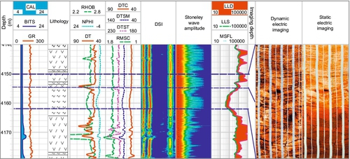
The acoustic and electric imaging logs provide high-resolution sidewall images and fine depiction of geological characteristics of subsurface formation fractures, rock textures, and beddings. In volcanic reservoirs, FMI imaging logs are widely used to identify fractures.
1 Imaging log response characteristics of fractures
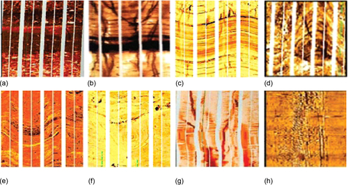
In an FMI imaging chart (Figure 6.2), open fractures have low resistivity and usually show black-colored, sinusoidal or irregular lines or narrow stripes. The characteristics of filled fractures are related to the conductivity of infilled material. If the filler conductivity is low, filled fractures will show white, sinusoidal or irregular lines or stripes. If the filler conductivity is high, filled fractures will be black sine-curves or stripes. The height difference between the peak and valley of a sine curve is related to the fracture dip angle: the greater the dip angle, the greater the height difference.

2 FMI imaging log identification model
Highly conductive fractures, high-resistivity fractures, microfractures, and induced fractures can be identified effectively using the sine-curve theoretical fitting method [4] to establish an FMI imaging log interpretation model for volcanic rock fractures (Figure 6.3, Table 6.1).

Table 6.1
FMI Imaging Log Response Characteristics of Different Fractures
| Fracture Type | Major Geological Origin | Imaging Logging Characteristics | |||
| Color | Shape | Grouping Characteristics | Extended Distance | ||
| Highly conductive fracture | Structural fracture, columnar joint, dissolution fracture, sutured fracture | Black | Sine-curve type | Multigroup | Long |
| High- resistivity fracture | White | Sine-curve type | Multigroup | Long | |
| Microfracture | Blast fracture, contraction fracture, weathered fracture | Black | Irregular | Chaotic, nongroup | Short |
| Induced fracture | Stress-released fracture, hydraulic fracture | Black | 180-degree symmetrical feathered and chevron shapes | Single group | Long |

1) Highly conductive fractures
Highly conductive fractures consist of mostly open structural fractures, columnar joints, and dissolution fractures. The direction or orientation of these fractures depends on the regional tectonic stress field, and pores and cavities are developed in as bead strings along fracture faces. In an FMI imaging chart, they show black sine curves or narrow stripes with multigroup characteristics and long extensions (Figure 6.3a, Table 6.1).
2) High-resistivity fractures
These fractures refer to early structural fractures and columnar joints, which are closed or filled with high-resistivity materials. In an imaging chart, they show white sine curves or narrow stripes with multigroup characteristics and long extensions (see Figure 6.3b, Table 6.1).
3) Microfractures
This group comprises blast fractures, contraction fractures, and weathering fractures with a limited extension, as well as structural fractures that are locally filled or closed. They serve primarily as connections between pores in the reservoir. In an FMI imaging chart, microfractures show black irregular lines or narrow stripes with a short extension, without any typical sine-curve or group characteristics. Therefore, these fractures usually do not fit the sine-curve theory (see Figure 6.3c, Table 6.1).
4) Drilling-induced fractures
These fractures are non-natural fractures generated during drilling and related to crustal stress. The fracture orientation follows the direction of the maximum horizontal principal stress. In the imaging chart, they show feathered or chevron-shaped black symmetrical curves (180 degrees) appearing along the sidewall with single-group characteristics and a long extension (see Figure 6.3d, Table 6.1).
3 Fracture identification through image logging
Natural fractures are classified and picked up based on the identification model, the result of lithology identification, and the discrimination between true and false fractures. Induced fractures are identified based on an analysis of regional structural stress. The characteristics of various fractures in wells are ascertained to establish a basis for determining fracture shapes, spatial distribution, and fracture parameters.
1) Fracture identification based on lithological constraints and identification
Different types of major fractures are developed in different lithologies. Structural fractures and dissolution fractures are developed in all lithologies; contraction fractures occur mainly in effusive volcanic rocks; blast fractures occur in explosive volcanic rocks and near volcanic conduit facies; and sutured fractures occur in the hot base surge subfacies of explosive facies. Therefore, lithological constraints for fracture identification are established through lithological identification.
2) Identification of natural fractures through image logging
Natural fractures can be ultimately identified according to petrogenetic differences and the response characteristics of image logging and by determining the differences between natural fractures and geological features (e.g., layer interfaces, fault planes, shale stripes, bedding planes, rhyolitic structures, and hydraulic fractures):
1. Layer interface. This refers to the interface between two sets of formations. In an image logging chart, layer interfaces are marked by a group of nearly parallel conductivity anomalies. Compared with fractures, layer interfaces have the characteristic of uniform, continuous, and integral distribution, and they do not intersect each other. Usually there is a color transition between layer interfaces and formations (Figure 6.4a).
2. Shale stripes. Unlike fractures, the high conductivity anomalies of shale stripes are generally parallel, regular, and have clear boundaries. Even after severe tectonic deformation, the change in their widths will not be significant (Figure 6.4b).
3. Beddings. Beddings appear in groups within a certain range. In general, low-angle beddings are parallel to each other and demonstrate extremely good regularity between lines (Figure 6.4c).
4. Faults. There is displacement in the formations at both sides of fault plane, but there is no displacement in the fracture system (Figure 6.4d).
5. Rhyolitic structure. In an image logging chart, rhyolitic structures are deformed sine curve in shape with a visible disturbance trace, but the line is smooth. The long axis of elongated vesicles is aligned with the direction of magmatic flow (Figure 6.4e).
6. Perlitic structure. As the name implies, this is a unique structure for perlite and is marked by arcuate or concentric cracks; these cracks divide acidic volcanic glass into many small balls. In imaging logs, perlitic structure shows dark-colored, arcuate, or concentric lines under a high-resistivity background. Therefore, it can be easily distinguished from fracture zones (Figure 6.4f).
7. Heavy mud hydraulic fractures. These are the hydraulic fractures caused by the imbalance between drilling fluid and structural stress, resembling stress-release fractures, and generally developed in two to four groups (Figure 6.4g).
8. Scratches of drilling tools. These scratches are caused by the friction between drilling tools and the well sidewall, without sine-curve characteristics in the imaging chart, and their cutting depth is shallow (Figure 6.4h).
3) Classified pickup of natural fractures and induced fractures
On the basis of a clear understanding of the differences between natural fractures/induced fractures and other similar geological features, natural fractures and induced fractures are picked up in the classification process using special image logging interpretation software and the human-machine interaction approach. This lays the foundation for fracture parameter calculation and the evaluation of fracture development, fracture effectiveness, and fracture orientation.
6.2.2 Identification of fractures through conventional logging
Natural and induced fractures with different dip angles are identified by qualitative log analysis and semiquantitative fracture index calculation according to the abnormal response characteristics of fractures in conventional logging curves.
1 Conventional log response characteristics of fractures in volcanic rocks
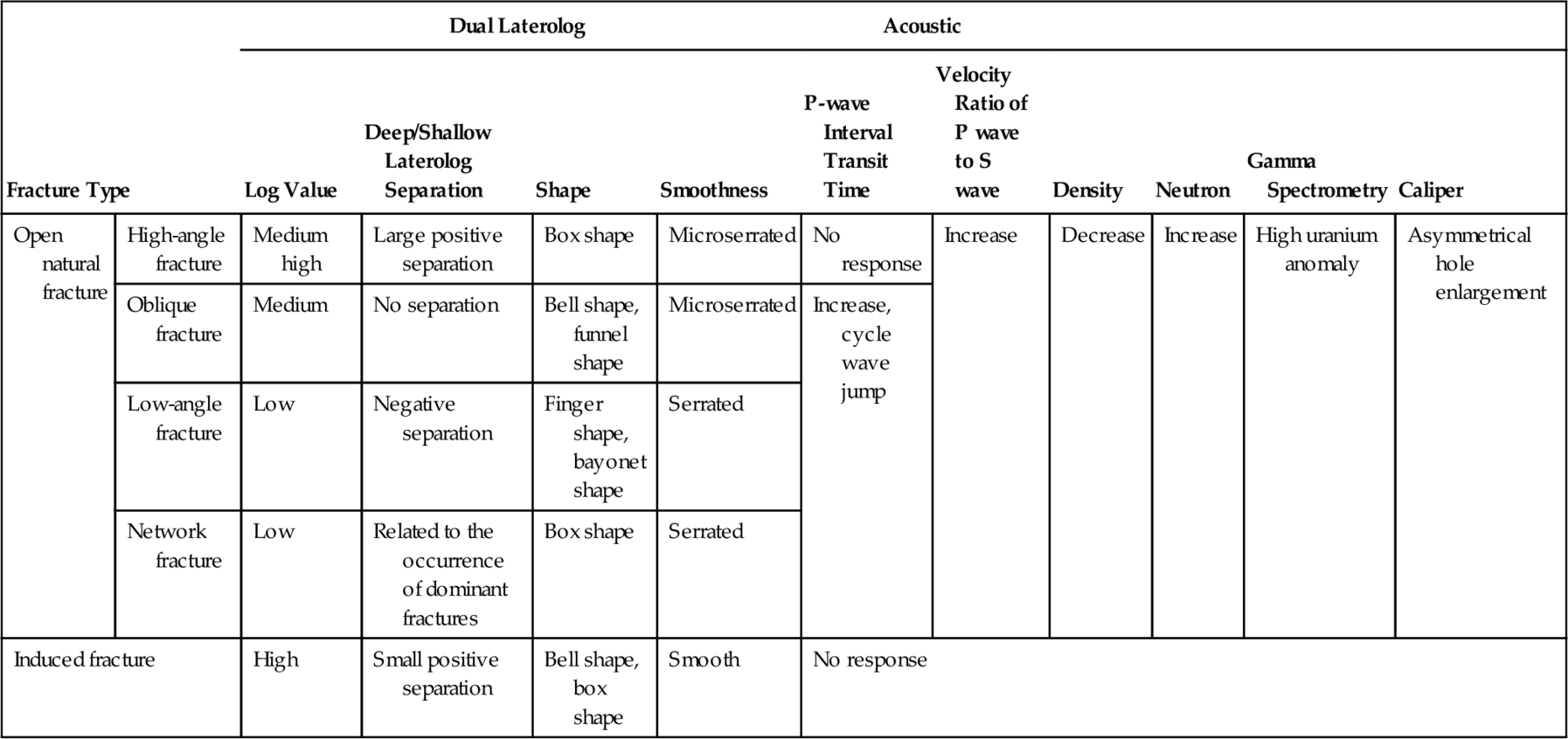
The radioactivity, physical properties, and conductivity of a rock formation are measured through conventional logging to indirectly reveal the characteristics of fracture development in volcanic rocks. Conventional log data can be calibrated by descriptive logs of cores and analysis of the logging response characteristics of cored intervals, which will help reveal the conventional logging characteristics of fractures in volcanic rocks (Table 6.2) and establish the typical fracture log identification model.
Table 6.2
Conventional Log Response Characteristics of Fractures in Volcanic Rocks
| Fracture Type | Dual Laterolog | Acoustic | |||||||||
| Log Value | Deep/Shallow Laterolog Separation | Shape | Smoothness | P-wave Interval Transit Time | Velocity Ratio of P wave to S wave | Density | Neutron | Gamma Spectrometry | Caliper | ||
| Open natural fracture | High-angle fracture | Medium high | Large positive separation | Box shape | Microserrated | No response | Increase | Decrease | Increase | High uranium anomaly | Asymmetrical hole enlargement |
| Oblique fracture | Medium | No separation | Bell shape, funnel shape | Microserrated | Increase, cycle wave jump | ||||||
| Low-angle fracture | Low | Negative separation | Finger shape, bayonet shape | Serrated | |||||||
| Network fracture | Low | Related to the occurrence of dominant fractures | Box shape | Serrated | |||||||
| Induced fracture | High | Small positive separation | Bell shape, box shape | Smooth | No response | ||||||
1) Dual laterolog
A dual laterolog provides resistivity curves that reflect undisturbed formations and fracture-invaded zones.
In deep and shallow laterolog resistivity curves, open fractures result in a decrease in resistivity values and a difference between the deep and shallow laterolog resistivity values. Thus, high-angle fractures (dip angle > 75 degrees) have a positive separation (i.e., RLLD > RLLS (recorded laterolog shallow)), low-angle fractures (< 60 degrees) have a negative separation, and oblique fractures (60 ~ 75 degrees) have a small separation or no separation (see Table 6.2) [5,6].
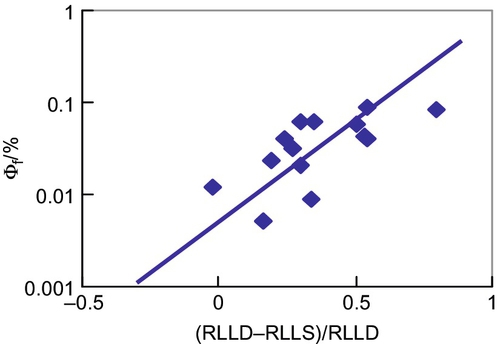
In volcanic reservoirs, high-angle structural fractures are predominant. In dual laterolog curves, fracture-bearing intervals are characterized by decreased resistivity value, and positive separation between deep and shallow laterologs. Figure 6.5 is a crossplot of the surface porosity of fractures in cored intervals, which shows a difference between deep and shallow laterolog resistivity values [(RLLD−RLLS)/RLLD] in the XX gas field. This figure shows that the more developed the fractures (the greater the surface porosity), the smaller the RLLD, and the larger the RLLD−RLLS values. This implies that high-angle fractures are responsible for the decrease in resistivity and the increase in positive separation between deep and shallow laterolog resistivity values.
2) Acoustic log
There is no response for high-angle fractures in P-wave interval transit time curves. Instead, the response increases in low-angle fracture and network fracture intervals, and even “jumping cyclic waves” occur in these intervals. At the same time, fractures cause an increase in the acoustic travel time of S waves and Stoneley waves but a decrease in their amplitude. The amount of change is greater than that of P waves [5,7], and the velocity ratio (Δts/Δtc) of P wave to S wave increases (see Table 6.2).
Figure 6.6 is the crossplot of surface porosity of fractures in the cored interval and the P-S ratio of acoustic travel time in the XX gas field. This figure demonstrates that the P-S ratio of acoustic travel time increases as the surface porosity of fractures increases, but it is affected by fluid properties.

3) Compensated density and compensated neutron logs
A compensated density log reflects the total porosity in rocks, whereas a neutron log detects the hydrogen content in formations. Fractured intervals have reduced density and increased neutron log values, but natural gas causes a decrease in both density and neutron values (see Table 6.2). Under identical conditions, therefore, the level of fracture development is determined with the direction of relative change in density and neutron log values [5,7].
4) Gamma spectrometry log
Fluid is more active in fractures than in matrix pores, which facilitates abnormal uranium enrichment and intensifies the radioactivity in formations [5,7]. The degree of fracture development can be determined by analyzing the uranium enrichment characteristics (see Table 6.2).
5) Caliper log
In dual- (or multiple-) caliper log curves, well radius enlargement and ROP change occur when the caliper detects an open fracture. The more developed the fracture, the more significant the caliper response. Therefore, an asymmetrical hole enlargement is the primary basis for fracture identification in dual-caliper (or multiple-caliper) log curves (see Table 6.2).
2 Conventional logging identification model for fractures in volcanic rocks
A conventional logging identification model for fractures in volcanic reservoirs is established through an analysis of log response characteristics, after the conventional log is calibrated by core description logs and imaging logging identification [12].
1) High-angle fractures
In conventional log curves, high-angle fractures commonly have a smooth box shape and are characterized also by moderate amplitude values and a large separation of deep and shallow laterologs, small interval transit time, high density, and significant neutron log values.
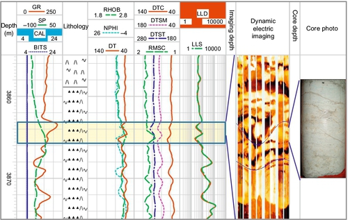
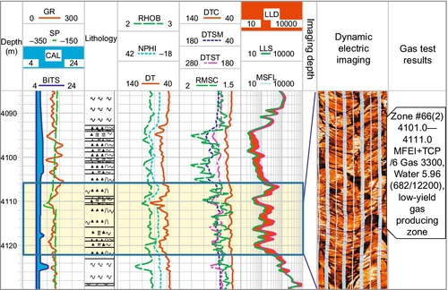
The brecciated lava reservoir interval in 3705 to 3744 m of Well XX8 is a typical example (Figure 6.7). Core description and imaging log identification information indicate that this interval has the characteristics of abundant vesicles and dissolution pores, good matrix properties, and its fractures are mostly high-angle structural fractures. Its conventional log curve shows a smooth box shape. Its average value of deep and shallow laterolog resistivity is 38 Ω·m and 21 Ω·m, respectively. The acoustic transit time is 71 μs/ft on average, with neutron porosity of 14% on average and rock density 2.32 g/cm3 on average. As the gas test in the studied interval shows, its natural production rate of natural gas is up to 23 × 104 m3/d, its producing pressure differential is 8 MPa, and no water is produced. A short-period production testing for 30 days shows that the gas production rate was maintained at 15 × 104 m3/d, the water production rate increased from 6.3 m3/d to 98 m3/d, and the water-gas ratio stabilized at 6.6 to 6.8 m3/104 m3, implying that the water from the lower water zone has risen up into the gas zone along high-angle fractures.

2) Low-angle fracture
Low-angle fractures have a bayonet shape in conventional log curves, with low amplitudes in resistivity curves, a large negative separation between deep and shallow laterologs, large interval transit time, small density, and large neutron values.
The tuff-bearing volcanic brecciated reservoir in 3863 to 3866 m of Well XX5 is a typical example (Figure 6.8). Core description and imaging log interpretation indicate that a group of low-angle fractures (3 ~ 4) is developed in this interval. Conventional log curves show a bayonet shape. Their average values of deep and shallow laterolog resistivity are 44 Ω·m and 50 Ω·m, respectively, which are lower than those of the surrounding rocks. A negative separation is also observed. Their interval transit time is 64 μs/ft on average, and their neutron porosity has an average of 5%, which is slightly higher than that of the surrounding rocks. Their rock density has an average of 2.58 g/cm3, which is slightly lower than that of the surrounding rocks.
3) Network (netlike) fractures
These are formed by intercrossing fractures with various occurrence patterns, indicating a high degree of fracture development. In conventional log curves, the intervals with network fractures have serrated and box shapes and a low-amplitude resistivity curve. Whether deep and shallow laterologs show positive or negative separation depends on the occurrence of dominant fractures. Their interval transit time is long, neutron porosity is high, and the density is small.
The brecciated lava reservoir interval in 4108 to 4122 m of Well XX9 is a typical example (Figure 6.9). The imaging log indicates that this interval is rich in predominantly high-angle network fractures. Conventional log curves are serrated or box shaped. Their average value of deep and shallow laterolog resistivity is 230 Ω·m and 95 Ω·m, respectively, and a positive separation is observed. Their interval transit time has an average of 65 μs/ft, and their neutron porosity is 4% on average—higher than that of the surrounding rocks. Their rock density is 2.52 g/cm3 on average—lower than that of the surrounding rocks. As shown by the gas test in this interval, the natural production rate of natural gas is 0.33 104 m3/d, and the water production rate is up to 5.96 m3/d.
4) Stress-release fractures
Stress-release fractures are developed mainly in tight intervals where tectonic stress is not easily released. In conventional log curves, they have a smooth box shape. They are characterized by a high amplitude resistivity curve, a small positive separation or no separation in deep and shallow laterolog resistivity, a short interval transit time, low neutron porosity, and high rock density values.
The dacite formation in 3980 to 3985 m of Well XX401 is a typical example (Figure 6.10). The imaging log indicates that this interval has abundant 180-degree symmetrical stress-release fractures. Its conventional log curve has a smooth bell shape. The average value of deep and shallow laterolog resistivity is 1452 Ω·m and 1244 Ω·m, respectively, and a small positive separation is observed, albeit larger than that of the surrounding rocks. Their interval transit time has an average of 52 μs/ft, and their neutron porosity is 3% on average—lower than that of the surrounding rocks. Their average rock density is 2.57 g/cm3—higher than that of the surrounding rocks.

3 Identification of fractures through semiquantitative calculation of fracture index
According to the response characteristics of fractured intervals in conventional log curves, fractures are further identified by calculating indicative curves that reflect the degree of fracture development, using the curve combination technique.
1) Calculation methods
The calculation methods commonly used are as follows:
1. Secondary porosity method. In reservoirs dominated by high-angle fractures, the variation of interval transit time is small, whereas the rock density and neutron porosity are high. An indicator function that reflects the degree of high-angle fracture development is thus established:
Where
ϕND — neutron and density crossplot porosity (%);
ϕS — acoustic porosity (%).
2. Apparent pore structure index method. Fractures improve the flow pathways and electric conduction paths in reservoirs, and they cause the pore structure index to decrease. An indicator function that reflects the degree of overall fracture development is thus established:
Where
Rw — formation water resistivity (Ω·m);
Rt — original formation resistivity (Ω·m);
ϕ — matrix porosity (%).
3. Deep and shallow laterolog amplitude difference method. High-angle fractures cause an increase in the positive separation between deep and shallow laterolog resistivity. An indicator function that reflects high-angle fracture development degree is thus established:
Where
RLLD — deep laterolog resistivity (Ω·m);
RLLS — shallow laterolog resistivity (Ω·m).
4. Uranium anomaly index method. Fractures provide the migration pathway for various fluids, which become more active than in the matrix. Formations with abundant fractures have higher enrichment of radioactive uranium. A fracture identification indicator function based on gamma spectrometry is established:
Where
U — gamma spectrometry uranium curve (ppm);
Th — gamma spectrometry thorium curve (ppm).
5. Fracture probability function method. A comprehensive method of fracture probability function is established based on the preceding methods. This method will further amplify the log response of fractures and improve the congruence rate of fracture identification. The fracture probability function calculation formula is

Where
XFPR2 — the normalized curve of FPR2;
Xm — the normalized curve of m*;
XFPU — the normalized curve of FPU;
XFLPL — the normalized curve of FLPL;
W1–W4—the weighted coefficients for XFPR2, Xm, XFPU, and XFLPL.
6. Fracture development exponential function method. To reduce artificial errors, a fracture development exponential function curve that semiquantitatively evaluates fracture development is further established:
Where
2) Calculation results
A fracture indicative curve is established using the previously described methods. The relationship between the indicative curve and fracture parameters of FMI imaging logs is then determined. The adaptability of each method is analyzed here.
Calculation of fracture indicative curve using conventional logs
Secondary porosity (FPR2), the apparent pore structure index (m*), deep and shallow laterolog amplitude difference (FLPL), uranium anomaly index (FPU), fracture probability function (FIDX), and fracture development index (FID2) are calculated based on conventional logs using the preceding methods. Traces 8 to 13 in Figure 6.11 show that FPR2, m*, FIDX, and FID2 are generally consistent with the fracture development characteristics determined through image logging, and the correlation between FPU, FLPL, and imaging log interpretation results is poor. This implies a poor applicability or adaptability of the deep and shallow laterolog amplitude difference method and the uranium anomaly index method to the identification of fractures in volcanic reservoirs.

Applicability and adaptability
The applicability and adaptability of each method is analyzed by establishing the relationship between indicative curves and imaging log fracture parameters.
Based on calculated fracture indicative curves and the expression between each calculated curve and fracture parameters of the FMI imaging log, the adaptability of individual evaluation methods is analyzed.
In Well XX14, the thickness of volcanic rocks is approximately 400 m. Rhyolite, rhyolitic brecciated lava, rhyolitic tuffaceous lava, and rhyolitic volcanic breccia are encountered during drilling. Lithofacies include effusive facies, explosive facies, volcanic conduit facies, extrusive facies, and volcanic sedimentary facies. Therefore, this well can be regarded as highly representative of various lithologies. The calculation result of Well XX14 and analysis (Figure 6.12, Table 6.3) shows the following:
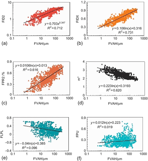
Table 6.3
Table of Adaptability Analysis of the Calculation Methods of Fracture Indicative Curves by Conventional Logs
| Method | Analysis of Relationship with Fracture Hydrodynamic Width via Imaging Logs | Correlated Thickness | Lithology | Lithofacies | |
| Expressions | Rt | ||||
| Secondary porosity method | y = 0.01ln(x) + 0.013 | 0.62 | 400 m | Rhyolite, breccia lava, tuffaceous lava, volcanic breccia | Effusive facies, explosive facies, volcanic conduit facies, extrusive facies |
| Pore structure index method | y = 0.22ln(x) + 3.193 | 0.62 | |||
| Deep and shallow laterolog difference | y = 0.04ln(x) + 0.385 | 0.1 | |||
| Uranium anomaly index method | y = 0.012ln(x) + 0.223 | 0.02 | |||
| Fracture probability function method | y = 0.105ln(x) + 0.316 | 0.71 | |||
| Fracture development index method | y = 0.703x0.346 | 0.73 | |||

1. The volcanic secondary porosity method. FPR2 increases with fracture development and correlates fairly well with the hydrodynamic width of fractures determined via imaging logs (Figure 6.12c), showing a good applicability and adaptability for this method.
2. The apparent pore structure index method. m* decreases with the degree of fracture development and correlates fairly well with the hydrodynamic width of fractures determined via imaging logs (Figure 6.12d), also indicating a good applicability of this method.
3. The deep and shallow laterolog difference method. FLPL increases with high-angle fracture development and correlates poorly with the hydrodynamic width of fractures determined on the basis imaging logs (Figure 6.12e); this method is highly affected by the variation of lithology, induced fractures, and fluid type, indicating poor applicability.
4. The uranium anomaly index method. FPU increases with fracture development and correlates poorly with fracture hydrodynamic width determined via FMI imaging logs (Figure 6.12f); this method is highly affected by the variation of lithology and sedimentary environment and thus is of poor applicability.
5. The fracture probability function method. FIDX increases with fracture development and correlates fairly well with fracture hydrodynamic width determined via imaging logs (Figure 6.12a); it shows somewhat improved results compared with single methods and offers good applicability and adaptability.
6. The fracture development index method. FID2 increases with fracture development and correlates fairly well with the fracture hydrodynamic width determined from imaging logs (Figure 6.12b); it has been improved somehow compared with single methods and offers good adaptability.
Among these six evaluation techniques, the methods based on deep and shallow laterolog difference and uranium anomaly index are shown to have a poor applicability or adaptability due to the impact of such factors as lithological change, induced fractures and fluid type variation; they are mainly suitable for qualitative analysis of volcanic reservoirs with stable lithology and significant difference of fluid activity. The other four methods offer a good applicability and adaptability and can be used to semiquantitatively evaluate the degree of fracture development.
3) Parameter characteristics of fracture indicative curve in volcanic rocks
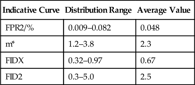
In the XX gas field, the calculation results of several wells have been statistically analyzed, and the results can be summarized as follows (Table 6.4): secondary porosity (FPR2) is between 0.009% to 0.082% with an average value of 0.048%, which means that the secondary action in volcanic reservoirs is not strong; the apparent pore structure index m* ranges between 1.2 to 3.8 with an average value of 2.3; the fracture probability function (FIDX) ranges between 0.32 to 0.97 with an average value of 0.67; and the fracture development index (FID2) ranges between 0.3 to 5 with an average value of 2.5.
6.2.3 Comprehensive identification of volcanic fractures in wells
Comprehensive studies involving geology, imaging logs, and conventional logs are carried out by integrating core description for the cored intervals, calibrating imaging log with cores, and calibrating conventional logs with cores and imaging logs. Fractures in volcanic reservoirs are identified in single wells according to the log response characteristics and fracture identification models.
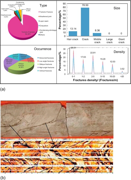
1 Describing fractures in cored intervals to calibrate imaging log data
Through fracture description for cored intervals, basic characteristics of fractures in volcanic reservoirs such as the type, configuration, and size are revealed. This helps calculate the fracture parameters, construct the volcanic reservoir fracture concept model (Figure 6.13a), and calibrate the imaging log (Figure 6.13b).
2 Identifying fractures with FMI imaging and integrated with core data to calibrate conventional logs
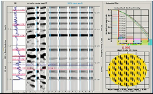
On the basis of the identification model for FMI imaging logs, fractures are picked up by type, piece by piece in noncored intervals, and conventional logs are jointly calibrated by core and image logging results (Figure 6.5, Figure 6.6, and Figure 6.14). As shown in Figure 6.15, traces 4 to 6 are the tadpole plots of highly conductive fractures, microfractures, and induced fractures, respectively. The figure shows that mainly oblique microfractures are developed in Well XX301, with upright induced fractures developed in its upper part.

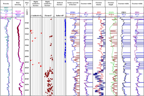
3 Qualitative identification of different fracture occurrences based on conventional log response characteristics
The high-angle, low-angle, network, and induced fractures are qualitatively identified with conventional log data, in accordance with the log response characteristics and identification model of induced fractures and fractures of different occurrences. In Well XX301 (Figure 6.15), the upper part (3950 to 4020 m) of the log curve shows mid-low amplitude values, a box shape, and good smoothness, suggesting mostly high-angle fractures; the lower part of the log curve shows high amplitude values and box and serrated shapes, pointing to mostly network fractures. The result of conventional log identification is largely consistent with the tadpole plot results using FMI imaging logs (tracks 4 to 6).
4 Semiquantitative evaluation of the degree of fracture development based on a fracture indicative curve derived from conventional logs
The degree of fracture development is semiquantitatively evaluated on the basis of the fracture indicative curve derived from conventional log data.
In Figure 6.15, traces 7 to 12 are the integrated curve of FPR2, m*, FPU, FLPL, FIDX, and FID2. Compared with the imaging log identification results, there is a general agreement between m* and fracture width. FPR2 and FLPL are basically consistent with the surface porosity of fractures; FIDX and FID2 are in agreement with the fracture width, whereas the effectiveness of FPU is poor. Therefore, the degree of fracture development can be semiquantitatively evaluated with conventional logs [8].
6.3 Interpretation and evaluation of volcanic reservoir fracture parameters
Fracture identification, as discussed in the previous section, involves interpreting fracture parameters, evaluating the degree of fracture development, fracture orientation, and fracture effectiveness, and determining the development characteristics of fractures in volcanic reservoirs, all of which will serve as the basis for fracture prediction.
6.3.1 Interpretation of fracture parameters
This mainly includes the interpretation of fracture density, fracture width, fracture porosity, and fracture permeability.
1 Calculation methods
1) Fracture density and fracture length
In this study, fracture density (FVDC) refers to the linear density, which is defined as the number of fractures per unit length (1 m) of the sidewall (unit: 1/m). Fracture density parameters are generally calculated from the fracture pickup in the acoustic or electric imaging chart. Other methods for fracture density calculation carry various degrees of uncertainty [9].
Fracture length (FVTL) is defined as the total fracture length per unit area (m2) of the sidewall (unit: m/m2 or 1/m). It is statistically determined by special software based on fracture identification.
2) Fracture width
Fracture width refers to the opening width of a fracture along the normal direction. It can be determined by acoustic/electric imaging and conventional logs.
The calculation method based on FMI imaging logs
Fracture width is generally smaller than the resolution of microresistivity image logging, which cannot be read directly. Instead, it has to be calculated indirectly on the basis of fracture color representation in the imaging log chart [10], and it is calculated using the following formula:
Where
ɛ — width of a single fracture (mm);
a, b — constants related to instruments, wherein b is close to zero;
A — the area of conductivity anomaly (mm2) caused by fracture;
Rxo, Rm — resistivity values of invaded zone and drilling fluid (Ω·m).
The width of fractures is different in a different part of the reservoir. Fracture width can be determined by one of the two methods according to the result of point-by-point calculation:
1. The average fracture width (FVA), which is defined as the average value of all the fracture trajectory widths per unit well interval (1 m)
2. The average hydrodynamic width of the fracture (FVAH), which is defined as the cube and extraction of cubic root of fracture trajectory widths per unit well interval (1 m), which can be regarded as a fitting for the fracture hydrodynamic effect
The calculation method based on conventional logs
Before acoustic or electric imaging log was invented, Sibbit and colleagues provided a method for fracture width calculation with a dual laterolog resistivity curve [6]. This technique first requires the judgment of fracture occurrence, followed by the following parameter calculations, respectively:
Network fractures: first determine the width of high-angle and low-angle fractures, respectively, and then sum them up,
Where
Cd, Cs, Cm — conductivity values of deep laterolog, shallow laterolog and mud (mS/m);
Cb— matrix conductivity (mS/m) can be read from tight intervals near the interpreted layer.
3) Fracture porosity
Fracture porosity is calculated with an acoustic/electric imaging log and a conventional dual laterolog:
1. The calculation method based on the FMI imaging log. For FMI imaging logs, fracture porosity (FVPA) is defined as the apparent opening area of fractures per unit area of coverage in imaging chart (unit: cm2/cm2), calculated using the following formula:
Where
FVPA — fracture porosity (cm2/cm2);
FVA — average fracture width (cm);
FVTL — fracture length (m);
CAL — well radius (cm).
2. The calculation method based on conventional logs. Fracture porosity is calculated with a dual laterolog curve using the following formulae:
Where
ϕf— fracture porosity (fraction);
Cw— formation water conductivity (mS/m);
mf— fracture pore structure index, which is related to width variations and the bending of a fracture, typical range 1 to 1.3;
Kr— fracture’s influence coefficient on shallow laterolog resistivity, which is related to fracture occurrence and development degree; typical range 1.1 to 1.3; values of 1.3 to 1.5 for reservoirs with poor fracture development.
4) Fracture permeability
Fracture permeability is divided into two types. The first type, referred to as intrinsic fracture permeability, only takes into account the conductivity of fracture for fluid flow, ignoring the condition of surrounding rocks. It is mainly affected by the fracture surface, the fluid flowing direction, and the intrinsic characteristics of fractures. Its typical expression is

For the second type, known as fracture permeability of fractured reservoirs, the fracture and its surrounding rocks are treated as a whole hydrodynamic unit. This permeability is related to the degree of fracture development and the connection between fracture and matrix pores, calculated using the following formula:
Based on fracture occurrences and their combination types, the fracture permeability is calculated based the following three models:

Where
Kif, Kf — the intrinsic permeability of fractures, fracture permeability (mD);
di, d — width of the i-th fracture, average fracture width (μm);
α, β — the angle of a fracture and fluid flowing direction (°);
nα, nβ — number of fractures in fracture group that form α and β angles with the fluid flowing direction (fractures);
ϕf — fracture porosity (fraction).
The calculation result of Formula 6.3.9 represents the sidewall fracture permeability [10], where the radial extension characteristics and bending degree of the fracture are not reflected. To better reflect the reservoir fracture permeability, Formula 6.3.9 is improved as follows:
Where
R — fracture radial extension coefficient.
When a the radial extension of a fracture is greater than 2 to 3 m, the fracture is approximately of infinite extension (R = 1); when its extension is 0.5 to 2 m, it is of medium extension (R = 0.8); when its extension is 0.3 to 0.5 m, it is of shallow extension (R = 0.4); and when its extension is less than 0.3 m, it is of extremely shallow extension (R = 0);
The mf value refers to the structural characteristics index of the fracture, which reflects the fracture width and the degree of bending. For wide fractures, mf = 1.0; for narrow fractures, mf = 1.3. The greater the mf value, the less a fracture contributes to permeability.
2 Calculation result
As an example from Well Block XX21, Figure 6.16 shows the interpretation of fracture parameters for Well XX21, with the following results: (1) with increased fracture development, there are greater values for the fracture density, width, surface porosity, and permeability; and (2) the result of conventional logging interpretation largely agrees with the FMI imaging log and is slightly better than the imaging log for the gas-bearing interval (3660 to 3720 m).

The calculation results indicate that Well Block XX21 has a maximum fracture density of 21.33 fractures/m, 4.38 fractures/m on average, but mostly (72%) in the range of 1 to 5 fractures/m; fracture length ranges between 0.01 to 22.63 m/m2, with an average value of 4.07 m/m2, but mostly (80.69%) 1 to 8 m/m2; fracture width attains a maximum of 510 μm, ranging between 0 to 60 μm, with an average of 23.5 μm, and microfractures being predominant; fracture porosity is 0.537% at maximum and 0.03% on average; and fracture permeability is 103 mD at maximum and 0.9 mD on average.
6.3.2 Evaluation of fracture development
The degree of fracture development can be used to evaluate qualitatively the fracture development conditions in volcanic reservoirs. The criteria for fracture development evaluation are established on the basis of fracture identification and fracture parameter interpretation. Fractures are evaluated zone by zone, and their degree of development in different intervals of volcanic rocks in wells are ascertained, thereby providing the basis for fracture prediction.
1 Criteria for evaluating the degree of fracture development
In the XX gas field, the evaluation criteria for fracture development in volcanic reservoirs are established on the basis of parameter sensitivity analysis, through selection of three parameters, including fracture density (FVDC) interpreted based on FMI imaging logs, the fracture development index (FID2) derived from conventional logs, and the percentage of fracture intervals in reservoir thickness (HELF) [8]. The degree of fracture development in volcanic reservoirs is classified into four levels (see Table 6.5):
Table 6.5
Discrimination Criteria of Fracture Development Degree (XX Gas Field)
| Fracture Development | HELF / % | FID2 | FVDC / (fractures/m) |
| Well developed | > 70 | > 2.5 | > 2.5 |
| Fairly developed | 1.5 ~ 2.5 | ||
| Ordinarily developed | < 1.5 | ||
| Fairly developed | 40 ~ 70 | 2 ~ 2.5 | > 2 |
| Ordinarily developed | < 2 | ||
| Fairly developed | 10 ~ 40 | 1 ~ 2 | > 3 |
| Ordinarily developed | < 3 | ||
| Undeveloped | < 10 | < 1 | < 0.5 |

1. Well developed fractures: HELF > 70%, FID2 > 2.5, FVDC > 2.5 fractures/m
2. Fairly developed fractures, which are composed of three cases:
If HELF > 70% and FID2 > 2.5, then FVDC ranges between 1.5 and 2.5 fractures/m.
If HELF ranges between 40% to 70% and FID2 ranges between 2 and about 2.5, then FVDC > 2 fractures/m.
If HELF ranges between 10% to 40% and FID2 ranges between 1 and 2, then FVDC > 3.0 fractures/m.
3. Ordinarily developed fractures, which are also composed of three cases:
If HELF > 70% and FID2 > 2.5, then FVDC < 1.5 fractures/m.
If HELF ranges between 40% and 70% and FID2 ranges between 2 and 2.5, then FVDC < 2 fractures/m.
If HELF ranges between 10% and 40% and FID2 ranges between 1 and 2, then FVDC < 3.0 fractures/m.
4. Undeveloped fractures:
2 Evaluating the degree of fracture development
Fracture development is evaluated interval by interval on the basis of fracture development evaluation criteria, with fracture density (FVDC) interpreted from imaging logs, the fracture development index (FID2) from conventional logs, and the fracture thickness percentage (HELF) determined comprehensively. This lays the foundation for fracture prediction.
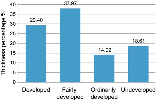
In the case study of Well XX21 (see Figure 6.16), the results of fracture development evaluation indicate (Figure 6.17) that, according to the four-level discrimination criteria, the fracture development in volcanic rocks of this well is ranked predominantly “fairly developed,” which accounts for 37.97% of total fractures; this is followed by the “well-developed” category (29.4%); “undeveloped” intervals only account for 18.6%. This suggests that the fractures in volcanic reservoirs of this well are fairly developed in general.
6.3.3 Evaluation of fracture effectiveness
Opening natural fractures are important for pore connection and fluid flow passages in volcanic reservoirs. The effectiveness of fractures in volcanic reservoirs is evaluated by geological analysis, acoustic log analysis, and comprehensive multiple-data analysis. This provides the basis for predicting effective reservoirs.
1 Geological evaluation
This line of evaluation is carried out mainly with respect to fracture width, infill characteristics, radial extension, and fluid flow capacity. Larger fracture width means longer extension, better openness, stronger fluid flow capacity for the fractures, and greater effectiveness. As is shown in the case study of Well Block XX21, comprehensive geological analysis revealed the following characteristics for the volcanic rock fractures in the study area:
1. The degree of openness is high: volcanic open fractures account for approximately 77% in cores; the highly conductive fractures and microfractures interpreted via FMI imaging log are predominantly open fractures (~ 95.7%). High-resistivity fractures account for only 4.3%.
2. The fracture width is 23.5μm on average, which is far greater than the throat diameter (0.14 μm on average).
3. The size of fractures is fairly large. Structural fractures and columnar joint fractures extend several tens of meters or even up to 100 meters. The average length of diagenetic fractures, such as blast fractures and interclast fractures, can reach up to 4.1 m/m2.
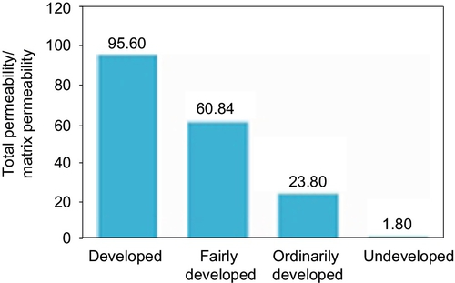
4. Fractures can significantly improve the fluid flow capacity of reservoirs. Diagenetic fractures mainly connect pore throats (Figure 6.18). Structural fractures are important as fluid flow channels. Thus, these fractures effectively improve the fluid flow capacity of volcanic reservoirs. In Well Block XX21 (Figure 6.19), for example, when fractures change from undeveloped to developed, the total permeability of volcanic reservoirs will increase by 1.8 to 95.6 times of the matrix permeability; therefore, fractures are crucial for improving the permeability of volcanic reservoirs.

2 Acoustic log analysis
The S-wave anisotropy of the orthogonal dipole acoustic log is one of the important methods for evaluating fracture effectiveness [11,12].
1) The fundamental principle
At a certain angle between the direction of particle vibration caused by the S wave and the fracture strike, the so-called S-wave splitting will occur—that is, the incident S wave splits into a fast S wave and a slow S wave, which have particles parallel and perpendicular to the fracture strike, respectively, vibrating and propagating upward along the borehole axis and traveling at different velocities. In fractured volcanic formations, therefore, the S-wave velocity of the dipole sonic imaging (DSI) log generally shows obvious azimuthal anisotropy. The S-wave anisotropy of the formation is measured by the orthogonal dipole technique. Stress-release fractures, other fractures, and faults are identified, and their strikes are evaluated tentatively by parameters such as energy-percentage anisotropy (OffEne), acoustic travel time anisotropy (SLOANI), and time-based anisotropy (TIMANI).
2) The evaluation method
Figure 6.20 is an example of fracture effectiveness evaluation through the integrated use of DSI anisotropy and the FMI imaging chart. In the left chart, the third trace shows the velocity and energy-percentage anisotropy of fast and slow S waves; the fourth trace shows the azimuth and error of fast and slow S waves. This chart demonstrates that this reservoir section has very strong anisotropy and a wide range of variation in fast S-wave azimuth, implying that the phenomenon causing such anisotropy has multiple distribution azimuths. In the FMI imaging log chart, the anisotropy is caused by multiple high-angle fractures of different azimuths, and both the width and extension range of fractures are quite large, suggesting that these are effective fractures. The right chart shows just the opposite. The fractures shown in the FMI imaging log chart have a small width with limited extension, thus being ineffective fractures. The anisotropic characteristics shown in the DSI log are inconspicuous.

Many factors affect rock anisotropy, including variations in lithology, directivity and changes in rock texture and porous structure, and lineation and distribution of rock constituents. On the basis of acoustic anisotropic analysis and other log data, therefore, the uncertainty of evaluation can be reduced through an integrative interpretation of fracture effectiveness.
3 Integrative analysis based on multiple log data
Different logging tools have different resolutions and detection depths, and different log data can be analyzed together, for example, high-resolution FMI imaging logs and other logs (e.g., Azimuthal resistivity imaging (ARI), array induction, DSI, and conventional logs) can be analyzed and compared with each other. Thus, the effectiveness of fractured reservoirs and the influence of fractures on reservoirs can be evaluated.
When fractures and the matrix are considered together, the fracture effectiveness will also depend on matrix pore development and pore-fracture combination characteristics. When matrix pores and effective fractures are developed and the pore-fracture combination is good, the fractured volcanic reservoirs will be effective. As shown in Figure 6.21, 17 fractures are picked up from the dacite formation at 4150 to 4156 m in Well XX9 based on the FMI imaging log, where the fracture density is 2.83 fractures/m. Nine fractures are picked up from the rhyolite formation at 4156 to 4162 m, where the fracture density is 1.5 fractures/m; conventional logs and DSI interval transit time curves demonstrate that the lower interval has good physical properties, has low resistivity (380 Ω·m), and contains effective fractured porous reservoirs, where fractures improved the fluid flow property of the reservoirs. The upper interval has poor physical properties and high resistivity (approximately 20000 Ω·m) and contains fractured volcanic reservoirs of poor accumulation capacity, where fractures only work as seepage channels.
Methods for evaluating fracture effectiveness also include correlation analysis of FMI and ARI, Modular Dynamic Tester (MDT) testing, Stoneley wave energy attenuation analysis, dual laterolog and conventional porosity log combined analysis, and so on.
6.3.4 Evaluation of fracture occurrence (configuration)
Fracture occurrence or configuration refers to fracture dip, inclination, and strike, and it is one of the major factors for optimizing the planning of development well grid pattern and the design of horizontal well trajectory. Fracture occurrence is generally evaluated using the paleomagnetic method and imaging log method.
1 Paleomagnetic method
Rocks record the direction of the geomagnetic field when they were formed, changes of the geomagnetic field since their formation, and the direction of the latest geomagnetic field. The theory of paleomagnetism suggests that the geomagnetic field has the characteristics of a geocentric axial dipole field (GAD field), the location of the geomagnetic pole as recorded by rocks is almost always near the geographic pole, and magnetic coordinates are largely consistent with geographic coordinates. Therefore, the geographic coordinates of a core sample can be determined by measuring its direction of magnetization [13].
1) Definition of core coordinates
As shown in Figure 6.22, a standard XYZ coordinate system is established as follows: first, mark a line through the center of a circle, which is the cross section of the core column; this line is parallel with a group of fractures, and it is defined as the x-axis (the virtual north direction); second, drawing a line along the length of the core as the z-axis. Then, extract a minicore 25 mm in diameter along the direction of the marked line (x-axis), and establish a corresponding coordinate system xyz in this tiny core. Therefore, the corresponding relationship between these two coordinate systems is
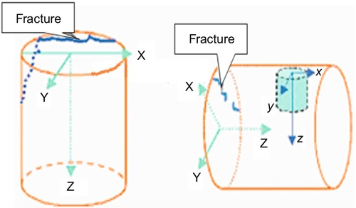

The occurrence of the fracture face within the XYZ coordinate system is known. The geographic coordinates of the tiny core sample can also be determined through measurements. The fracture occurrences data within the geographic coordinate system can be determined using this coordinate conversion formula.
2) Measuring the direction of magnetization of minicore sample
The magnetism that volcanic rocks obtained during a rock’s cooling moment is called the characteristic remanence (ChRM), which records the direction of the geomagnetic field when the rock was formed. The direction of the geomagnetic field when the volcanic rocks were formed can be determined by measuring the direction of their characteristic remanence. Once the characteristic remanence has been formed, it may decrease due to viscous demagnetization, or it may increase due to viscous remanence (VRM, which refers to the new intensity of magnetization continuously obtained below the Curie temperature). The ultimate direction of viscous remanence (which accounts for approximately 50% of the natural remanence) is consistent with the direction of the present geomagnetic field. Therefore, the direction of the present geomagnetic field (i.e., the present geographic direction) can be determined on the rock specimen through measurement of the direction of viscous remanence [14,15].
Viscous remanence can be erased under low-temperature demagnetizing conditions. Thermal demagnetization can be carried out at 12 temperature levels (i.e., 100° C, 150° C, 200° C, 250° C, 300° C, 350° C, 400° C, 450° C, 500° C, 530° C, 550° C, and 570° C). Each of the low-temperature components obtained through step-by-step thermal demagnetization below 300° C represents the direction of later viscous remanence, while each of the high-temperature components obtained above 300°C represents the direction of characteristic remanence. Figure 6.23 shows the demagnetization analysis of a core sample from the depth of 3100 m in Well XXSG2. Its natural remanent magnetization is 306 mA/m, which shows a uniform decrease from the demagnetization intensity of NRM –250° C to 70% of natural remanent magnetization, indicating approximately a viscous remanence demagnetization vector of NE 30 degrees. Beyond 300° C, as the demagnetization temperature rises, the remanent magnetization decreases gradually until it reaches 570° C when the remanent magnetization attenuates to 0.3 mA/m, indicating that the overall demagnetization direction of characteristic remanence remains at approximately NW 317 degrees with a dip angle of 61 degrees. This indicates that the direction of the magnetic field was NW 317 degrees when the volcanic rock was formed, whereas the direction of the present geomagnetic field is NE 30 degrees and the fracture direction is aligned largely toward the NE.

2 Imaging log method
Fracture occurrence can be determined by an image log chart. As shown in Figure 6.24, once fractures are identified, the height difference h between the peak and valley of the fracture sine curve and the average well radius d at the fractured interval are determined in the imaging chart. Thus, the dip angle θ of the fracture face can be expressed as [16]

The inclination of fracture planes can be read directly from the x-coordinate where the sine curve’s valley is located, and the fracture strike is perpendicular to its inclination.
The occurrence of a single fracture can also be read from the tadpole plot interpreted from the dip log and imaging log. The x-coordinate at the circular point of the tadpole is simply the fracture dip angle, whereas the azimuth at the tadpole tail point is the fracture inclination (see Figure 6.24). Azimuthal statistical analysis is performed for the target layer based on the determination of fracture occurrence. The predominant dip angle and inclination in the target layer are displayed by the azimuth frequency diagram (rose diagram; Figure 6.25).

6.4 Prediction of fractures in volcanic reservoirs
The results of fracture prediction provide an important basis for exploring high-quality volcanic reservoirs, optimizing well spacing, and optimizing horizontal well trajectories. Seismic response characteristics are analyzed on the basis of well identification, evaluation, and seismic calibration. Planar distribution of fractures is predicted by methods such as poststack seismic attribute analysis, prestack subazimuth processing and attribute analysis, and fracture parameter inversion.
6.4.1 Seismic response characteristics of fractures
The seismic reflection, wave impedance, and azimuthal anisotropic characteristics of fractures can be determined on the basis of a feasibility study on fracture prediction in volcanic rocks, through calibration of seismic data using fracture data from wells, and based on an analysis of seismic response of fractures, which therefore will lay a foundation for fracture prediction in volcanic reservoirs.
1 Feasibility of fracture prediction
Figure 6.26 is a geological model for vertical fracture simulation. The denudated top interface in its upper part is rugged and cut by minor faults. Fractures extend from the top interface into the model. The number of fractures indicates the developmental level of the fracture zone. Figure 6.27 is the seismic profile obtained through forward geological modeling. Comparison between these two charts shows almost no response on the left of the charts, but there is obvious amplitude, frequency, and phase anomalies on the right side; from left to right, as the degree of fracture development increases, the abnormal response in their seismic profiles becomes increasingly significant. This suggests that the seismic information cannot identify small single fractures but can identify fractured zones made up of small fractures.
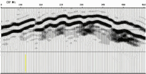
2 Characteristics of seismic reflection waveform
In the forward model (see Figures 6.26 and 6.27), fractured zones have the characteristics of poor continuity, weakened energy, and reduced frequency.
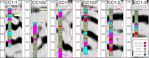
In seismic profiles, fractured zones often lead to changes in seismic reflection events [17]. As shown in Figure 6.28, in the fractured interval, the near-wellbore seismic trace event of Well CC1-1 corresponds to the wave trough and shows reflection characteristics of medium-weak amplitude and poor continuity; the event of the fractured interval in Well CC102 corresponds to the wave trough and shows reflection characteristics of medium-weak amplitude and poor continuity; the event of the fractured interval in Well CC1 corresponds to both the wave crest and trough and shows reflection characteristics of medium-weak amplitude and poor continuity; the event of the fractured interval in Well CC103 corresponds to the wave crest and shows reflection characteristics of medium-weak amplitude and poor continuity; and the fractured interval in Well CC1-2 corresponds alternately to wave crests and wave troughs and shows reflection characteristics of medium-weak amplitude and poor continuity. In seismic profiles, therefore, volcanic fracture intervals show reflection characteristics of weak energy and poor continuity.
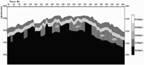
3 Wave impedance characteristics
In fractured intervals of volcanic rocks, a decrease in density and slowdown of acoustic propagation velocity are associated with a decrease in wave impedance. Figure 6.29 demonstrates the wave impedance variation characteristics of the fractured interval in Well CC103. In this figure, the fractured zone in volcanic reservoirs corresponds to a relatively low impedance, and the upper limit for the CC gas field is approximately 13200 (g/m3) · (m/s).

4 Anisotropic characteristics
Fractures have obvious anisotropic characteristics. If fractures in volcanic reservoirs are symmetrically arranged, the seismic attributes of fractured intervals will have distinct anisotropic characteristics [18]. In Figures 6.30 and 6.31, the results of prestack forward modeling for Well XX5 show that its fractures are distributed along the SN direction. It can be concluded from these figures that when the incident angle is small, the reflection amplitude of various azimuths remains the same; however, when the incident angle reaches 12 degrees or higher, the reflection amplitude of various azimuths becomes different, with larger incident angles correlated to greater differences. Therefore, fracture distribution can be predicted by detecting the anisotropy in seismic attributes.

The seismic response of fractures in volcanic reservoirs is simultaneously affected by multiple factors, such as lithological boundaries, faults, and the distribution of accumulation and seepage bodies. For fracture prediction, the results of log identification and evaluation must be fully utilized. The geological constraints must be used to improve the accuracy of prediction.
6.4.2 Method of post-stack seismic attribute analysis
The poststack seismic attributes for fracture prediction mainly include coherence, dip angle, amplitude, azimuth, and curvature.
1 Coherence analysis technique
The coherence analysis involves the calculation of dissimilarity among adjacent traces in seismic data volumes to construct coherent data volumes and to measure the similarity among multiple traces of seismic data. These data volumes are used to characterize the variation characteristics of continuity in seismic wave groups [19].
1) Coherence calculation method
The calculation method for seismic coherence is simple, using the following formula to calculate the correlation coefficient on the basis of the number of traces, the dip angle, and the time window of the given data volume:
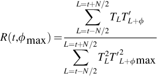
Where
R — coherence coefficient, which is a function of the time of seismic trace and the dip angle between two seismic traces;
t — time;
φ — dip angle, which is affected by azimuth and is not easily to be determined;
T, T′— seismic trace data pair.
The number of coherent traces involved in the calculation includes linear 3-trace, orthogonal 3-trace, orthogonal 5-trace, and orthogonal 9-trace. A greater number of traces will lead to a greater averaging effect. Multitrace coherence is used mainly to highlight major faults. In contrast, fewer coherent traces lead to a smaller averaging effect. Coherence of fewer traces is suitable for identifying minor faults or fracture zones. Selection of the coherent time window typically depends on the apparent period t of reflection waves in the seismic profile. Its value is usually in the range of t/2 to 3 t/2.
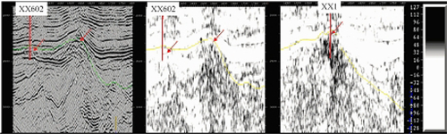
2) Prediction of fracture distribution using coherence analysis technique
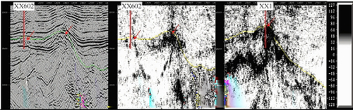
Figure 6.32 shows the T580-line migration profile, coherence profile, and T713-line coherence profile of the XX gas field. It demonstrates that the location in the migration profile with an event offset shows poor-coherence stripes in the coherence profile, whereas the location with good event continuity shows good coherence in the coherence profile. The area near Well XX602 with good coherency shows white stripes in the coherence profile, where fractures or faults are undeveloped, and the gas test confirms dry layers; the area near Well XX1 with poor coherency shows black irregular stripes in the coherence profile, where fractures or faults are developed, and the gas test shows commercial gas layers. This confirms that the coherence analysis technique can be used to identify fractured zones. However, the coherent data anomaly caused by lithological changes or poor data quality must be identified.
2 Margin-detection technique
Margin refers to the end of one region and the start of another. Margin detection treats seismic data as a special image and uses margin-detection operators and the maximum gradient or the zero-crossing point of a second derivative to extract image margins (location, direction, amplitude); therefore, the configuration of an abnormal change zone can be determined to achieve fracture prediction [20,21].
Figure 6.33 shows the T580-line migration and its margin-detection profiles and the T713-line margin-detection profile from the XX gas field. In the migration profile, the location with an event offset (arrow) corresponds to high (black) values in the margin-detection profile (the high yield zone in Well XX1), whereas the location with good event continuity corresponds to low (white) values in the margin-detection profile (the dry zone in Well XX602). This confirms that the margin-detection technique can also be used to predict fracture development zones effectively, although the prediction result still has some ambiguity, with fuzzy boundaries and low definition.
3 “Three-instantaneous” attribute analysis
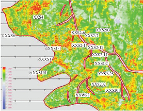
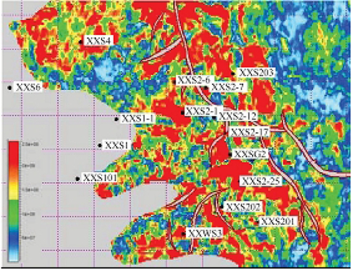
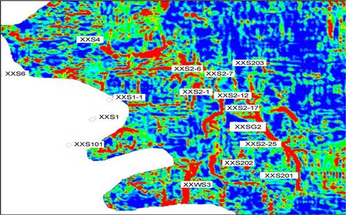
Petrophysical modeling experiments indicate that when the fracture opening decreases by 6.5 μm, the velocity of the seismic wave will increase by 4%, the quality factor by 70%, the amplitude by 1200%, and the dominant frequency by 44%. It is advantageous, therefore, to study fractures using the dynamical information (amplitude, frequency, and absorptive attenuation, etc.) of seismic waves. The technique of “three-instantaneous attribute analysis” predicts fractures on the basis of instantaneous amplitude, instantaneous frequency, and the instantaneous phase of seismic waves [22]. A good example for the application of this technique is found in the study of the YC3I top surface of Well Block XXS2-1 (Figures 6.34 through).


1) Instantaneous amplitude (A)
Instantaneous amplitude reflects the energy level of seismic reflection waves. The presence of pores, cavities, and fractures in reservoirs causes a decrease in reservoir velocity, reflection coefficient, and amplitude and energy of the reflection waves. Figure 6.34 demonstrates the presence of a low-amplitude areas in the southwest of Well Blocks XXS4 to XXS2-1, the east of Well XXS101, and the southeast of Well XXS2, which are in agreement with the poor-coherence area in the coherence analysis and the strong absorption area in the absorption coefficient analysis.
2) Instantaneous phase (Q)
The instantaneous phase reflects the continuity of seismic reflection waveforms. In terms of seismicity, minor faults and zones of pores, cavities, and fractures are characterized by event offsets, chaos, discontinuities, the increased number of event, and so on. In Figure 6.35, the areas of the chaotic instantaneous phase are mainly located in regions near Wells XXS4 to XXS2-1, Wells XXS to XXS2-25, west of Well XXS101, and near Well XXWS3. This is slightly different from the coherence areas and strong absorption areas.
3) Instantaneous frequency (F)
A rapid change in seismic wave frequency is related to factors such as stratigraphic pinch-outs and oil-gas-water interfaces. The presence of fractures in reservoirs causes the reservoir reflection coefficient sequence to change, which also results in abrupt changes in the instantaneous frequency, which is mainly reflected by the decrease of the instantaneous frequency. In Figure 6.36, areas of relatively low instantaneous frequency are mainly located in regions near Wells XXS1-1 to XXS2-7, north of Well XXS4, east of Well XXS101, and south of Wells XXS2-25 to XXS201. These correspond well with the poor-coherence areas and strong absorption areas.
4 Absorption coefficient analysis
Seismic wave absorptive attenuation is caused by the intrinsic viscoelasticity of the rock matrix (e.g., internal friction between particles and on fracture surfaces), the relative flow of liquids in porous rocks, the local saturation effect, and geometric diffusion. Fractures and their gas-bearing property will result in changes in seismic wave attributes such as velocity, amplitude, and frequency, thereby leading to absorptive attenuation of the seismic wave and further to changes in the seismic absorption coefficient.
1) Methods for calculating absorption coefficient
Under low-frequency conditions, when the seismic wave propagates in viscoelastic media, the absorption coefficient can be expressed with the following formula:

Where
η′— viscosity coefficient of viscoelastic media;
ω — circular frequency (Hz);
ρ — rock density (g/cm3);
κ — elastic modulus of rocks (N/m2);
λ, μ — lame coefficient.
The absorption coefficient is related to the rock density, elastic modulus, viscosity coefficient, and the seismic wave’s frequency. Assuming that c is a constant in viscosity coefficient η′ = c/ω and that P-wave velocity ν is used in place of the elastic coefficient, then the absorption coefficient can be simplified as follows:

Therefore, the effective absorption coefficient is inversely related to the cube of wave velocity. In other words, the sensitivity of the absorption coefficient in reflecting seismic anomalies far exceeds that of velocity, thus making it feasible to use the absorption analysis technique to predict fractures.
2) Prediction of fractures using absorption coefficient analysis method
There are two types of absorption coefficients: absolute absorption coefficient and relative absorption coefficient. Relative absorption coefficient refers to the absolute absorption coefficient divided by the background absorption coefficient, which highlights seismic energy absorption anomaly areas to better reflect the heterogeneity of geological bodies and as such is widely used to predict fractures.
Figure 6.37 is the planar distribution diagram of the absorption coefficient on the top surface of YC3I in Well Block XXS2-1, in which strong absorption areas are located mainly near Wells XXS2-6 to XXS2-1 and XXS2-17 to XXWS3; favorable reservoirs proven by drilling are mostly located in areas marked by high absorption coefficient values. This implies that the absorption coefficient method is suitable for predicting fractures in volcanic reservoirs.
5 Stress analysis technique
The tectonic strain and compressive strength of rock strata determine the occurrence and scale of faults and fractures. The formation strain in each tectonic phase is calculated using the kinematic and dynamic tectonic reconstruction method and by performing inverse and forward modeling of the structural history of rocks. By taking into consideration parameters such as formation thickness and lithology, the fractured zones and fracture direction in volcanic reservoirs can be predicted under the constraints of seismic attributes (e.g., coherence, amplitude attributes) [17,23,24].
Figures 6.38 and 6.39 show the planar distribution of formation strain and open fractures on the top surface of YC3I in Well Block XXS2-1 of the XX gas field, in which the areas of high formation strain values are mainly located near the fault zones north of Well XXS2-6 and secondarily west of Wells XXS2-1, XXS2-25, XXWS3, and XXS101. This indicates that faults and structures are important in controlling fracture development and distribution and that open fractures are mainly located near faults and in structural high areas.
6.4.3 Prestack fracture prediction method
The seismic reflection of fractured zones has anisotropic characteristics. The degree of fracture development and fracture orientation can be effectively predicted through prestack seismic subazimuth processing and attribute analysis [25–27].
1 Anisotropic characteristics of volcanic reservoirs
Earth media has three types of anisotropy: intrinsic anisotropy, secondary anisotropy, and wave length anisotropy. Volcanic rocks have secondary anisotropy caused by lithological change, rhyolitic structure, fractures, and the like. In an anisotropic medium, if the elastic properties in all directions at a given plane are the same and the axial directions of all points in the perpendicular plane are all mutually parallel, this plane is called an isotropic plane, the axis perpendicular to the isotropic plane is called the axis of symmetry (Figure 6.40), and the elastic medium for the isotropic plane is called the transversally isotropic (TI) medium. When the TI medium’s axis of symmetry coincides with z-axis, it is called a VTI medium, such as thin interbeds cyclically deposited in a horizontal bedded medium. When the TI medium’s axis of symmetry coincides with the x-axis or y-axis, it is called an HTI medium or an expansion anisotropic medium. For example, the volcanic reservoirs with vertical fractures generated by tectonic stress are isotropic longitudinally but anisotropic transversely.

2 Prediction principle
Prestack fracture detection techniques recognize fractures based on the rule of azimuthal anisotropy of 3D P-wave attributes in the HTI medium, including the VVA, AVA, and FVA techniques.
1) VVA technique
The VVA technique identifies fractures with the characteristics of reflection wave velocity that changes with the incident azimuth. As shown in Figure 6.41, the P-wave velocity of the HTI medium is [26,27]

Where
α — p-wave velocity during vertical incidence;
δ(v), ε(v)— Thomsen parameters of the HTI medium;
ϕ — azimuth, which is the angle between the ray plane (i.e., the source-receiver azimuth) and the HTI medium’s axis of symmetry.
From Formula 6.4.4, for horizontal fractures, ϕ = 90 degrees and Vp0 = α, where the Vp0 value is the maximum.
For vertical fractures,
where the Vp0 value is the minimum; and the azimuth and velocity between them range between these two values.
When directional vertical fractures are present in the formation, the velocity along different azimuths will show an ellipse: the velocity is the maximum when it propagates along the fracture strike. The velocity is the minimum when the propagation is perpendicular to the fracture strike. Mallick, Craft, and colleagues believe that the long axis direction of the azimuthal ellipse represents the fracture strike and the ellipticity represents the fracture density.
2) AVA technique
AVA refers to the change of amplitude with azimuth. The AVA technique identifies fractures based on the characteristics of reflection amplitude that change with incident azimuth. Rüger provided a P-wave reflection coefficient formula for HTI media [26,27]:
From the preceding discussion, it can be concluded that the P-wave reflection coefficient of the HTI medium is related not only to the P-wave velocity, S-wave velocity, shear modulus, and Thomsen anisotropy parameters δ and ɛ, but also to the incident azimuth and incident angle. Rüger believes that for a large fixed incident angle, the change of the HTI medium’s P-wave reflection coefficient with incident azimuth shows elliptical characteristics, the ellipticity being proportional to fracture density, and the long axis azimuth of the ellipse representing the fracture azimuth [26,27].
3) FVA technique
The seismic scattering theory for fractured reservoirs suggests that the seismic wave’s high-frequency attenuation caused by fractures results in the anisotropy of the seismic reflection frequency. The FVA technique detects fractures by the azimuthal anisotropy of 3D P-wave frequency attributes. Like VVA and AVA, the long axis direction of the ellipse of frequency changes with the azimuth and represents the fracture strike, and the ellipticity represents the anisotropic intensity of the frequency, which is related to the density of open fractures.
The frequency attributes related to attenuation mainly include the following: (1) the maximum amplitude frequency (i.e., the frequency corresponding to the maximum amplitude) is related to the fluid—the greater the seismic wave attenuation, the lower the frequency; (2) the frequency corresponding to 85% of seismic energy (i.e., the corresponding frequency when the energy in the analysis time window reaches 85% of total energy; Figure 6.42) is related to fluid properties—the greater the seismic wave attenuation, the smaller the frequency value; and (3) the frequency attenuation gradient refers to the intensity of frequency attenuation within unit distance (or time) and reflects the absorption of P-wave propagation by the strata—the stronger the strata’s absorption, the greater the gradient value.
3 Prediction method
The fracture-sensitive seismic attributes can be optimized based on the anisotropic characteristics of the prestack seismic attributes of fractures, through subazimuth processing of prestack seismic data, and hence the degree of fracture development and azimuth can be predicted. This is discussed next using the XX gas field as an example.
1) Forward modeling
Forward modeling is an important approach for building petrophysical models and analyzing the seismic anisotropic response characteristics of the models, which is the basis for predicting fractures with prestack seismic data.
HTI media are formed in volcanic reservoirs where vertical fractures are developed, and five independent elastic coefficients are needed to describe the anisotropic characteristics. Random anisotropic media will be formed by stratum inclination caused by tectonic movement, and 21 elastic coefficients are needed to describe the anisotropy. On the basis of the fractured reservoir geological model and elastic media model, and using rock P-wave velocity, S-wave velocity, and density parameters, the prestack forward model is built to calculate the elastic tensor and anisotropy-equivalent Thomsen indices, to calibrate the response of prestack seismic reflection along individual azimuths, and to determine the relationship between seismic reflection amplitude and fractures. The calculation results provide seismic responses to fractures at near-borehole seismic traces, including prestack amplitude variation with offset (AVO) characteristics, prestack AVO characteristics of individual azimuths, and the changes in AVO characteristics with azimuth influenced by fractures.
Figure 6.43 shows the results of prestack forward modeling for Well XX5 at different incident angles. The designed fracture direction is true north, where the azimuth is 0 degrees toward the true east direction. The first trace in the diagram is the gamma curve. The second trace shows synthetic traces and seismic records. For the third trace, the upper section simulates how the reflection amplitude of volcanic reservoirs changes with the changing incident angle with different azimuths, and the lower section is the amplitude ellipse simulated by reflection amplitudes of individual azimuths at different incident angles. Figure 6.43 demonstrates the following:
1. When the incident angle is small, it is equivalent to the vertical incidence of seismic waves, where the reflection amplitude of various azimuths has no difference; the larger the incident angle, the bigger the difference. Therefore, prestack fracture detection requires data acquired using large incident angles (i.e., large offsets).
2. With a fixed azimuth, the amplitude of the reflection wave is the maximum when it is perpendicular to the fracture direction (an incident angle of 0 degrees), decreases as the incident angle increases, and becomes the minimum when it is parallel to the fracture direction (90 degrees).
3. The difference between reflection amplitudes at various azimuths increases with the incident angle, and likewise the ellipticity of reflection amplitudes increases with the incident angle. When the incident angle is ≤ 3 degrees, the ellipticity is 1. At an incident angle of 12 degrees, the ellipticity is 1.006. When the incident angle reaches 24 degrees, the ellipticity is 1.026. At an incident angle of 27 degrees, the ellipticity is 1.033.
The incident angle in the target layer of the field survey system in the XX gas field is between 2 degrees and 13.5 degrees, without significant azimuthal differences. The requirements of prestack fracture detection in processing must be ensured as much as possible.
2) Prestack subazimuth processing of fractures
Prestack subazimuth processing of fractures is an important part of prestack fracture detection. The processing procedure is as follows.
Preliminary processing
This step includes denoising, deconvolution, amplitude compensation processing, and so on. The main processing parameters include common midpoint (CMP) bins 25 m × 50 m, number of record trace 1920, and sampling rate 1 ms, recorded length 6 s, and datum level 120 m, replacing speed 1600 m/s.
Prestack conventional processing
This step focuses on velocity selection and residual static correction. Velocity selection depends on whether the energy of the velocity spectrum is concentrated and whether there is an obvious trend in velocity change. Moreover, the first arrival muting and spike pulse energy depression of large amplitude must be performed, and spectrum whitening must be used to improve the data resolution.
Subazimuth processing
Subazimuth processing is the most important step in prestack fracture detection. It is affected by uneven azimuth distribution, survey system offset, and the raw data interval times. On the basis of the actual situation in the XX gas field, the azimuth division scheme is determined by the method of azimuth division with unequal spacing (Table 6.6). At the same time, the range of offset is restricted at 200 to 1600 m, for the following reasons: (1) near-offset data come from near-vertical incident seismic waves and cannot reflect the azimuthal AVO characteristics of the fracture media; (2) the azimuth distribution or seismic data volume offsets are uneven, with unequal azimuth being used for division and uniformization processing being performed in bins; and (3) the bin cover times cannot be too large because some bins will have to take a detour far away, but the cover times should not be too small either because the stack quality will deteriorate. It is generally appropriate to use the cover times of 25.
Table 6.6
Azimuth Division Table
| Range of azimuth/(degrees) | 0 ~ 41.4 | 41.4 ~ 68 | 68 ~ 90 | 90 ~ 112.3 | 112.3 ~ 138.6 | 138.6 ~ 180 |
| Average azimuth/(degrees) | 20.7 | 54.7 | 79 | 101.2 | 125.5 | 159.3 |

Figure 6.44 is the processed profile of different attributes at different azimuths, and the results of subazimuth processing show that the structures have a normal shape, and the signal-to-noise ratio (SNR) and resolution satisfy the fracture detection requirements.

3) Prestack fracture prediction methods
Method selection
The application of various methods on the volcanic rock reservoirs of the XX gas field within the 0 to 20 ms time window range produced four types of distribution maps of anisotropic intensities (Figure 6.45). Among these, the warm tones indicate a strong anisotropic intensity and highly developed vertical fractures, and cold tones indicate a weak anisotropic intensity and less developed vertical fractures. The correlation analysis of fracture characteristics of the drilled target layer (Table 6.7) indicates that among the four attributes, the “quantile frequency of seismic energy” offers the highest congruence rate of up to 80%, and the remaining three methods are relatively poor, with a congruence rate of 60%. Therefore, the “quantile frequency of prestack seismic energy” attribute is selected for predicting fracture development characteristics of volcanic reservoirs.

Table 6.7
Table of Matching Information on Fracture Development in the Upper Interval of Cycle I in Volcanic Rocks of the XX Gas Field within a 0- to 20-ms Time Window
| Well Name | Fracture Density/(Fractures/M) | Quantile Frequency of Seismic Energy | Attenuation Gradient | Dominant Frequency | Amplitude |
| 601 | 4.5 | Match | Unmatch | Unmatch | Unmatch |
| XX1 | 1.9 | Match | Unmatch | Match | Unmatch |
| XX6 | 4.45 | Match | Match | Match | Match |
| XX5 | 0 | Match | Match | Match | Match |
| XX502 | 3.7 | Fair match | Match | Unmatch | Match |
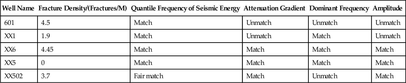
Fracture prediction
On the basis of prestack subazimuth processing of seismic data and the changes in quantile frequency of seismic energy with azimuth, the volcanic rock fracture development and orientation in target layers are predicted horizontally.
Figure 6.46 shows the following results of fracture prediction in the research area. Figure 6.46a illustrates the magnitude of ellipticity of the azimuthal ellipse for the “quantile frequency of seismic energy” attribute, where warm tones indicate a large ellipticity and a high fracture density, and cold tones depict a small ellipticity and a low fracture density. Figure 6.46b shows the result of directional rose-diagram statistics within the elliptical space of the same attribute. This result indicates the azimuth of fractures, and the size of the statistical grid is 100 m × 100 m. In this figure, the fault trends represented by black polygons are predominantly NNW and secondarily NNE; fractures are mostly developed to the left of faults along the NNW direction, and the fracture direction is mostly EW and NNW.
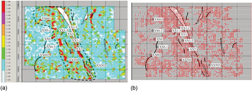
4) Analysis of controlling factors
The major controlling factors in prestack fracture prediction include the following.
Geological characteristics of volcanic gas reservoirs
The geological factors leading to the anisotropy in strata are complex. In addition to directionally arranged fractures, the factors also include lithological change, anisotropy inside rocks, fractures, folds, and so forth. Petrophysical research at Stanford University (in the United States) suggests that mudstone has a stronger anisotropy than sandstone. Fracture prediction based on the anisotropy in volcanic reservoirs is ambiguous. In practice, it must be combined with geological studies in order to enhance the geological guidance.
Acquisition and processing factors
Prestack fracture detection utilizes 3D data to acquire azimuthal anisotropy of P-wave attributes. Theoretically, it requires accurate seismic incident data from at least three different azimuths. Therefore, the acquisition process must satisfy wide-azimuth acquisition, as well as ensure uniform time coverage along individual azimuths and uniform distribution of offsets at individual azimuths. In actual practice, it is a challenging task to meet these requirements. During data processing, therefore, multiple methods must be used to determine processing parameters so as to minimize the negative impact of acquisition factors.
6.4.4 Fracture parameter inversion methods
The statistical relationship between fracture parameters and wave impedance is established on the basis of wave impedance inversion. 3D wave impedance data volumes are converted into fracture development parameter volumes with specific geological significance. These steps facilitate the effective prediction of fracture distribution in volcanic reservoirs [28].
1 Analysis of the statistical relationship between fracture parameters and wave impedance
From a petrophysical perspective, there are certain relationships among wave impedance, resistivity, and the fracture development index. The relationship between wave impedance and the fracture development index can be obtained through crossplot analysis.
1) The relationship between fracture index RTC and wave impedance
The dual laterolog resistivity is fairly sensitive to fractures. On the basis of crossplot analysis of wave impedance versus deep and shallow laterolog resistivity values (Figure 6.47), the conversion formula fitting wave impedance to resistivity is obtained:

The formula converting deep laterolog to shallow laterolog is obtained through statistics:
The formula converting deep/shallow laterolog to fracture index RTC is as follows:
Where
RLLD, RLLS — deep laterolog resistivity, shallow laterolog resistivity, (Ω·m);
Im — wave impedance [(g/cm3) · (m/s)];
RTC — fracture index; the larger the RTC value, the more developed the high-angle structural fractures.
2) The relationship between fracture development index FID2 and wave impedance
The degree of fracture development is positively correlated with the fracture development index but inversely correlated with wave impedance. Correlation analysis (Figure 6.48) indicates that there is a negative linear relationship between fracture development index FID2 and wave impedance:

Where
FID2 — fracture development index;
Im — wave impedance [(g/cm3) (m/s)].
2 Wave impedance inversion
Conventional wave impedance inversion includes basic processes such as fine horizon calibration, wavelet extraction, initial model setup, and volume inversion. The inversion results yield volcanic reservoir wave impedance 3D data volumes.
3 Fracture parameter inversion
There is a good statistical relationship between RTC and wave impedance, but a poor statistical correlation between FID2 and wave impedance. Therefore, the following two types of inversion are adapted.
1) RTC inversion
This inversion is performed in three steps: (1) the previously mentioned expressions are used to convert relative wave impedance data volume obtained through sparse-spike inversion into deep and shallow laterolog resistivity data volume; (2) a geological model is built by interpolating deep and shallow laterolog resistivity curves, followed by frequency band compensation performed on the model to correct its low-frequency and high-frequency components, and finally absolute deep and shallow laterolog resistivity inversion data volumes are generated; and (3) RTC data volumes are ultimately obtained through conversion in accordance with the relationship between deep/shallow laterologs and RTC.
2) FID2 inversion
This inversion is performed in the following steps using the so-called double inversion approach (Figure 6.49): (1) an apparent acoustic curve is established by the statistical relationship between the fracture development index (FID2) and acoustic wave; (2) reservoir horizon calibration and wavelet extraction occur; (3) the inversion model is constructed; (4) the pseudo-impedance volume derived from the characteristic parameters of fractures is obtained through constrained inversion of the model; and (5) fracture development index 3D data volume is obtained through constrained inversion of the characteristic parameter curve for the fractures.

4 Fracture prediction
In the volcanic reservoir of YC3I in Block XXS2-1, fracture distribution is predicted through RTC inversion. The results indicate (Figure 6.50) that areas with high RTC values are mainly located near Well XXS4, along the XXS2-1 to XXS2-6 to XXS2-7 to XXS203 zone, near XXS202 to XXS2-25, as well as northwest and north of the study area. Drilling operation has since confirmed that these are fracture-developed zones.

In the volcanic reservoir of YC1I in Block XX8 and Block XX9, the results of FID2 inversion indicate (Figure 6.51) that areas marked by high FID2 values correspond to the development of horizontal strips, present in a total of five plays, including XX9 to XX902, XX3 to XX14, XX8 to XX801, XX301, and XX7 to XX3. These fractured zones in the volcanic reservoir have also been confirmed by subsequent drilling.

6.4.5 Methods for optimization of volcanic reservoir fracture prediction
Many fracture prediction methods are available. The fracture prediction method suitable for a particular volcanic reservoir is optimized through assessment of the advantages, disadvantages, contributing factors, and seismic data requirements of different prediction methods, with reference to the volcanic reservoir characteristics.
1 Characteristics of fracture prediction methods
Different fracture prediction methods are based on different principles and, therefore, their advantages and disadvantages are also different (Table 6.8).
Table 6.8
Comparison of Volcanic Reservoir Fracture Prediction Methods
| Prediction Technique | Major Advantage | Disadvantage | Influencing Factors | |
| Poststack seismic attribute analysis | Coherence analysis | Sophisticated technique, simple operation | Strong ambiguity | Lithological boundary, fault |
| Margin detection | Intuitive image identification | Fuzzy boundary, low definition | Lithological boundary, fault boundary | |
| Three-instantaneous attribute | Simple, direct, and reliable | Strong ambiguity | Internal structure, fluid types | |
| Absorption coefficient | Sensitivity is high, result is good | Gas influence is high | Pore structure, fluid flow, local saturation effect | |
| Stress analysis | Theoretical basis is reliable | Paleostructure restoration too complex | Formation thickness, lithology, structure history | |
| Prestack seismic prediction method | Subazimuth processing, ambiguity is reduced, development degree and direction are also predicted | Strict requirements for wide-azimuth acquisition of seismic data; heavy workload for long time coverage | Data acquisition and processing; other anisotropic characteristics of formation | |
| Fracture parameter inversion method | Well-constrained, easy to implement | Dependence on level of correlation between fracture parameters and seismic information, uncertainty high | Relationship between inverted parameter and wave impedance; thickness and distribution of sedimentary rocks | |
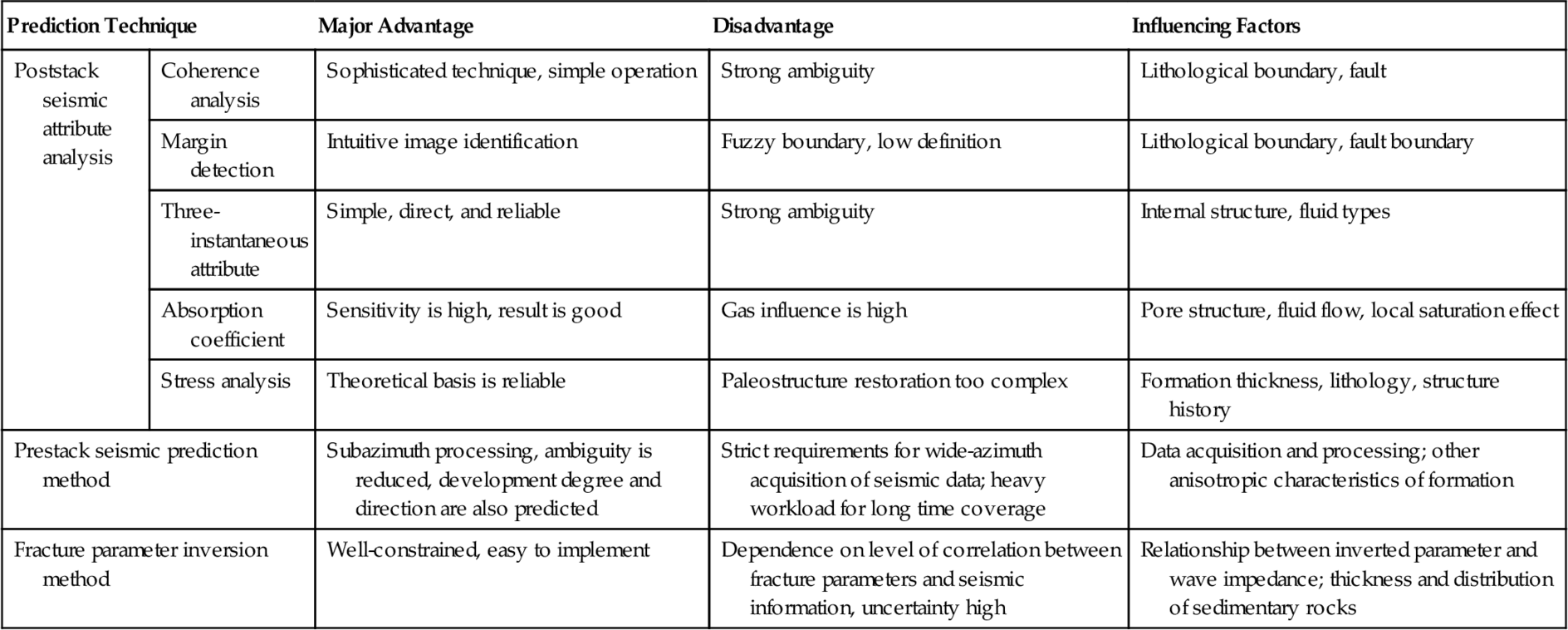
1) Method of poststack seismic attribute analysis
1. Coherence analysis. This is a sophisticated attribute analysis technique. It predicts fractures based on the dissimilarity between adjacent seismic traces. Its advantages include easy extraction of attributes and simple operation. However, it is strongly affected by factors such as lithological boundaries and faults, with strong ambiguity.
2. Margin-detection technique. This method predicts fractures through image analysis, which is visual, intuitive, and suitable for detecting large faults. For fracture prediction, however, the boundaries tend to be fuzzy, of low definition, and easily affected by faults, lithological boundaries, and so on.
3. Three-instantaneous-attribute method. This method detects fractures directly with P-wave dynamical information (amplitude, frequency, phase), which is simple, direct, and reliable. However, this method is significantly affected by internal structure and fluid type in volcanic rocks, also resulting in strong ambiguity.
4. Absorption coefficient method. This method predicts fractures based on the principle that fractures will intensify the seismic wave absorptive attenuation. Its advantages include high sensitivity and a good prediction result. However, it is strongly affected by the gas-bearing nature of formations and is also influenced by many other factors such as porous structures, fluid flow, and local saturation effect, also leading to strong ambiguity.
5. Stress analysis. This method predicts fracture distribution by calculating the strain generated during tectonic activities using the kinematic tectonic reconstruction method. It has a reliable theoretical basis and offers a good prediction result. However, the tectonic reconstruction process is complicated, thus the prediction result is affected by factors such as formation thickness, lithology, and structural history, resulting in some uncertainty.
The method of poststack seismic attribute analysis requires high-quality poststack 3D seismic data.
2) Prestack seismic prediction methods
These methods predict fracture distribution by the “quantile frequency of seismic energy” attribute based on fracture anisotropy. Their advantages include the ability to reduce ambiguity through subazimuth processing. However, subazimuth processing needs a huge data volume and a long cycle time, and it requires the data volumes acquired via wide azimuth and processed via subazimuth. At the same time, the prediction result is easily affected by other anisotropic media (such as mudstone) in the formation.
3) Fracture parameter inversion method
The spatial distribution of characteristic parameters of fractures is predicted using seismic inversion techniques, which are simple to implement and offer a high well-point congruence rate. However, their prediction effectiveness depends on the level of correlation between fracture parameters and seismic information, leading to a high degree of prediction uncertainty. They are also strongly affected by the thickness and distribution pattern of sedimentary rocks, leading to further increase in uncertainty. The fracture parameter inversion methods require high-quality 3D seismic data.
2 Optimization of volcanic fracture prediction methods
Volcanic fracture prediction methods under different conditions are optimized based on the guidelines of employing the highest-quality seismic data and most advanced prediction methods available, taking into consideration characteristics of volcanic rocks such as highly variable rock types, complex internal structures, complex fluid distribution, and a great variety of fracture types:
1. If the field seismic data are collected with wide-azimuth and processed by prestack subazimuth and amplitude preserving method, the prestack fracture prediction method can be used to predict fracture-developed zones for improving prediction accuracy.
2. If only conventional poststack seismic data are available, several methods, such as stress analysis, absorption coefficient, and multiattribute coherence, can be used together to predict fracture-developed zones with reduced ambiguity.
3. Poststack seismic inversion of fracture parameters is now considered an auxiliary method for the two techniques.
In summary, when seismic methods are used to predict fracture developed zones, the seismic data must go through high-resolution, high-SNR, and high-definition processing to meet the requirements of fracture prediction.
6.5 Technological applications
The characteristics and distribution patterns of fractures in volcanic reservoirs can be ascertained using various fracture identification and prediction techniques. This will provide the basis for predicting favorable reservoir zones, optimizing well locations, and analyzing bottom water coning.
6.5.1 Prediction of favorable reservoir zone in volcanic gas reservoirs
In volcanic reservoirs, fractures are important for connecting pores and enhancing fluid flow pathways. As the degree of fracture development increases, the permeability of volcanic reservoirs increases by 1.8 to 95.6 folds compared to matrix permeability (see Figure 6.19). As a result, fractures constitute a major controlling factor for the permeability of volcanic reservoirs. Favorable reservoir zones in volcanic gas reservoirs can be predicted on the basis of fracture distribution and the distribution characteristics of effective reservoirs. This lays the foundation for locating high-yielding wells.
6.5.2 Well location optimization
Fractures determine the well grid pattern, well spacing, and horizontal well trajectories. For development wells in fractured gas reservoirs, irregular well patterns are generally used: (1) high-yielding wells should be placed to a maximum in fracture-developed zones; (2) wide well spacing should be adopted along the direction of fractures, and narrow well spacing along the direction perpendicular to fractures; the more developed the fractures and the longer the fracture half-length, the higher the irregularity of the development well pattern; and (3) the trajectory of horizontal wells is generally perpendicular or oblique to fractures. In the XX, CC, and DD gas fields, 12 horizontal wells were drilled on the basis of the prediction of fractures in volcanic rocks, and all of which have met their expected goals, with excellent results.
6.5.3 Determination of vertical distribution of fractures for analysis of bottom water coning
Fractures are important communicating mechanisms between gas layers and bottom water. When the production pressure differential exceeds a given value, the bottom water may migrate upward along fractures, resulting in water production from gas layers. The vertical distribution of fractures can be assessed through fracture identification and evaluation, which will provide the basis for the evaluation of bottom water coning.