Chapter 3

The Contemporary and the Everyday Life of Wireless Optical Communication

3.1. Basic principles

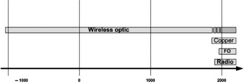
The wireless optical communication systems were the first to be used (Figure 3.1) and, due to technological innovations, they become attractive, mainly because of the lack of produced or suffered radio interference and, especially, from the ever-increasing demand of the data rate.

Before presenting the daily and contemporary applications of wireless optical communication, we define some basic principles and the different modes of propagation.

3.1.1. Operating principle

3.1.1.1. Block diagram

Wireless optical communications refer to the use of light propagation in the field of optics with free space as a transmission medium.

An example of the principles of operation is detailed in Figure 3.2 with various technical modules present in an optical wireless in emission (Tx) and in reception (Rx). At the transmission (Tx), from digital data received by a computer or a server via a suitable interface (D-Tx), a digital and analog electronic processing (El-Tx) is performed to adapt the signals to electrical-optical converter (Ot-Tx). This converter is usually a light-emitting diode (LED) or a laser. Using the divergence optical device (Op-Tx), a beam is emitted more or less divergent to the receiving device. At the reception (Rx), part of the received beam is optically concentrated (Op-Rx) to be focused on the optical-electrical converter (Ot-Rx), which is a photodiode. Electronic processing (El-Rx) is inversely made to adapt the signals to the interface (D-Rx). This communication is also possible in the opposite direction and provides a two-way communication.

In most cases, a monitoring software is supplied with devices. This software allows us to configure the connection and obtain qualitative and quantitative information of the various modules.

One of the main parameters in the characterization of a wireless optical device is the distance: it varies depending on the equipment from a few tens of centimeters (IrDA equipment) to several tens of thousands of kilometers (intersatellite link). The rate and type of application recommended is also essential. The proposed data rate starts from a few kilobits per second or Kbps (103 bit/s) to several terabits per second or Tbps (1012 bit/s). The different applications are discussed later in this chapter.

3.1.2. The optical propagation

There are several propagation characteristics in optical wireless links. The propagation between the emitting source and the receiving cell can be carried out in three systems (hybrid systems combine one and/or the other of these characteristics):

– line of sight (LOS);

– wide line of sight (WLOS);

– propagation by diffusion with specular and diffuse reflection (DIF) also sometimes referred to as non-line of sight (NLOS).

3.1.2.1. Line of sight propagation — LOS

This is the simplest link and best-known system for point-to-point (PtP) communication. In this case, the transmitter and the receiver are manually or automatically pointed (tracking), one toward the other to establish a link (Figure 3.3).

The LOS from the transmitter to the receiver must be clear of obstructions and the majority of the transmitted beam is directed toward the receiver. This is the configuration of the majority of outdoor wireless optical communication systems (free-space optic — FSO) and optical communication systems between computers or devices (IrDA). These links can be created temporarily for a session of data exchange between two users (or computer systems), or permanently set in a local network.

This type of propagation is characterized by:

– the absence of any obstacle in the space between the transmitter and the receiver;

– high power efficiency, due to the low divergence emission (a few degrees). Much of the signal is routed to the receiver;

– a less important receiver sensitivity to ambient light because field of view (FOV) of the receiver is lower;

– better resistance to multipath and, by extension, to intersymbol interference (ISI), again because of a low FOV of the receiver;

– an available throughput only function of the link budget and not from the dispersion of multipath and problems related to ISI, the latter is similar to an echo phenomenon.

These LOS systems, therefore, have very limited flexibility and high sensitivity to the obstacles and are particularly suited to a PtP configuration.

Unfortunately, these narrow beams do not provide a large coverage for communication. To remedy this problem, two approaches are possible and are described below.

In the first approach, a manual or automatic pointing device [MAM 98] is installed, the response times are fast, but the costs are currently incompatible with the creation of a common network.

In the second approach, a multiple transmitting/receiving device with multiple coverage angles is used [PAR 01]. In this multisectoral or cellular approach (Figure 3.4(a)), it is possible to ensure high coverage while maintaining high data rates [WIS 97].

The implementation of multiple transmitter and receiver couples, each couple having a specific and different angle of coverage, can be achieved by the introduction at the reception of an angular diversity [CAR 00, OME 09], presented in Figure 3.4(b). Another more compact approach [YUN 92] is shown in Figure 3.4(c) for the reception part, for example. It consists of several receptors (matrix array) arranged on a flat surface and associated with a converging lens [KAH 98]. This device allows an imaging reception where the detector will be different depending on the angle of the incident beam [OBR 03]. This second solution offers a significant miniaturization of optronics modules.

3.1.2.2. Wide line of sight — WLOS

Configuration for WLOS (Figure 3.5) is characterized by an emitter with a larger divergence angle, so more coverage, and receivers with a wide angle of reception. This extended coverage makes it easier to overcome an alignment between the transmitter and the receiver, but the downside is that only a small fraction of the emitted power is received by the receiver. So there is a significant degradation of the link budget.

In addition, the implementation of the high divergence emitter leads to the appearance of reflections on walls and objects in a room. This results in the possible appearance of multiple paths arriving on large FOV receptors. From a certain distance between the transmitter and the receiver, it is a side effect that restricts the data rate and the quality of the transmission; this is known as ISI.

The ISI is an unwanted phenomenon for a wireless optical communication, which is manifested as a signal distortion. Indeed, the symbol transmitted at time T-1 and having bounced off a wall, for example, can become a noise and affect the transmitted symbol at time T. This is equivalent to an echo phenomenon and makes communication less reliable. Orthogonal frequency-division multiplexing (OFDM) and discrete multitone (DMT) modulation are solutions in the field of data processing that reduce the ISI (see Chapter 9).

WLOS links are more adapted to point-multipoint (PmP) communication. A typical example is an access point that allows for communication with receiving devices in the covered area [SMY 95] and the best-known product is the remote control device.

3.1.2.3. Diffusion propagation (DIF) and controlled diffusion

In a diffuse system, the connection is always maintained between any transmitter and any receiver in the vicinity, by reflecting the optical beam on surfaces such as ceilings, walls, and furniture (Figure 3.6). In this case, the transmitter and the receiver are not necessarily directed toward each other, the emitter uses a highly divergent beam, and the receiver has a large FOV, so that the direct path is not required.

Such a mode of operation ensures a communication, regardless of the obstacles or the person preventing the direct path. However, the penalty of the diffuse transmission is that the capacity is reduced compared to the LOS system. This is mainly due to losses that are typically over 100 dB and a multibeam receiver, which create ISI.

The signal-processing solutions are required to reduce this phenomenon, but an approach known as controlled diffusion can also solve this problem.

The first controlled diffusion device was proposed in the late 1970s (Figure 3.7) by Gfeller and Bapst [GFE 79] at a rate of 1 Mbps. Then a data rate of 50 Mbps was reported in the 1990s by Marsh and Kahn [MAR 96]. This system illuminates the walls and ceiling with controlled lighting, coupled with a receiver that accepts the reflected beam in a limited angular aperture. It aims to combine the robustness of the diffuse system with high data rates.

Many publications have proposed such geometries [DJA 00], including the use of transmitters that illuminate small areas on the ceiling [YUN 92]. They are used in conjunction with a narrow FOV receiver to capture the different incident beams with similar optical path.

The latter two regimes are well suited to the application of wireless local area networks such as WLAN (wireless local area network) and WDAN (wireless domestic area network) because users do not need to know the location and orientation of the various communicating devices.

3.1.3. Elements of electromagnetics

The transmission of information can take different forms. The use of transfer of information from the information that can convey the electromagnetic waves is one of the richest possibilities. More details about electromagnetic waves are discussed in the next section. This section will consist of a classic reminder of electromagnetic waves. We discuss the Maxwell equations that control the propagation of these waves in different environments, then we recall the expression of the energy carried by these waves, and, finally, we present the propagation rays models.

3.1.3.1. Maxwell’s equations in an unspecified medium

The propagation of electromagnetic waves is conducted by Maxwell’s equations that are [BRU 92, COZ 83, VAS 80]:

These equations allow us to treat the propagation of electromagnetic waves in any medium. If we consider the propagation in free space which is the subject of this book, the previous set of equations is simplified. Indeed, the wave propagation takes place in a homogeneous environment and without charge ( = 0 and ).

In addition, we consider the transmission medium as isotropic, and linear or non-dispersive:

The simplest case is vacuum propagation where (F/m) and (H/m). In a specific medium, we will call /₀ the relative permittivity _r and /₀ the relative permeability _r.

To address this problem, we consider the case of sinusoidal time. In other words, we look after solutions that exist for t = −∞ to +∞ and assume that the fields and inductions vary sinusoidally with time and at the same pulsation . For example, the real electric field denoted by can be written as:

To simplify the calculations, it is generally preferred to use the following complex notation:

In the rest of this section, we use the complex notation, the field will simply be noted .

3.1.3.2. Propagation of electromagnetic waves in an isotropic medium

The goal of this part is to characterize the waves propagating in a linear and isotropic homogeneous medium. The medium is homogeneous if the permittivity is constant. Let us consider the simplest case, i.e. the propagation in a homogeneous medium without any electrical charge. Using the complex notation, this can be written as:

From the four preceding relations, the two following equations are deduced:

These two relations are generally known as the equations of propagation. Their analytical resolution shows that:

is the wave vector or propagation vector. It expresses the spatial frequency of the wave. The spatial period is linked to through .

, , and form a right-handed orthogonal trihedral of vectors. In other words, if the electric field propagates along the direction given by its wave vector , the associated magnetic field has a single direction. The real fields and vary sinusoidally with time. Their dependence on the distance is shown in Figure 2.1. For a propagation in a homogeneous, dielectric, and isotropic material, and , as well as their associated complex notations, lie in a plane normal to the direction of propagation. In this case, the electromagnetic vibration is said to be transverse.

From the previous relations, the phase of the wave can be written in the form:

The phase velocity, i.e. the speed necessary for remaining at a constant phase, is:

For a wave propagating in a medium:

3.1.3.3. Energy associated to a wave

The energy balance is one of the most significant parameters for the link. Until now, we have considered plane waves extending in all the planes normal to the direction of propagation. For optical links, the beams will be limited laterally. We shall recall here the expression for luminous flux through surfaces in the case of plane waves.

To calculate the energy carried by a wave, let us first recall that the electromagnetic energy present in a volume V is expressed by the relation [BRU 92]:

The energy density is given by:

In the case of a plane wave propagating in a perfect medium, it can be shown that the electrostatic energy is equal to the magnetic energy. The electromagnetic energy density is therefore:

Let us now consider the luminous flux through an uncharged homogeneous surface, normal to the direction of propagation, where the normal to the surface is parallel to the -axis. Let us consider the amount of energy during time dt = dz/, where is the speed of light in the medium considered. If the electric and magnetic fields are linearly polarized along Ox and Oy, it can be shown that the energy flux through the plane is equal to the flux of a normal vector given by [BRU 92]:

The Poynting vector is written as:

The instantaneous energy associated with the wave cannot be measured due to the fact that the frequency of light is about 10¹⁵ Hz, and the detectors measure only the average energy. Indeed, only the energy average over a period T is observable:

The average flux of the Poynting vector through a surface corresponds to the average energy carried by the wave through this surface.

NOTE. — Here again, it is necessary to be careful depending on whether the real or complex notation of the electromagnetic fields is used [VAS 80].

3.1.3.4. Propagation of a wave in a non-homogeneous medium

The plane waves described previously give the ideal case of an infinite, homogeneous, linear, and lossless medium. The case of wave propagating in air is close to this ideal case. Of course part of the electromagnetic energy propagating in the atmosphere will be absorbed by molecules in the air; the absorption process will be described in detail in Chapter 5. In a bounded medium, as is the case in an optical fiber or waveguide, it is necessary to take Maxwell’s equations regarding the differences between the media into account. The equations of propagation will no longer assume the simple form given by equation [3.8]. Since a purely analytical solution is not always available, it is necessary to use numerical algorithms for the resolution of the propagation equations of an electromagnetic wave in the system under consideration. Let us mention some algorithms such as the finite difference time-domain (FDTD) method, the beam propagation method in time domain (BPM), and the finite element integration method.

3.1.3.5. Coherent and incoherent waves

In free-space propagation, the diffraction and reflection processes generate several waves that interfere with one another (Figure 3.9). If two waves have a phase relation, i.e. they are coherent, the fields will be summed in amplitude and phase. The resulting field depends on the phase difference between the waves. If the two waves are incoherent with respect to one another, i.e. if there is no phase relation, the intensities still sum up. Thus, it is important to consider the phase relation between the detected signals.

Figure 3.9 shows the pattern at the detector level where two light beams will be added, one that has spread in a direct line (a) and another that has reflected on a surface roughness (b), and 2 is the FOV of the beam.

There is a more complete account of coherence and interference phenomena in the references given in the preceding section. Here, we shall only mention a few properties defined for plane waves, as well as some definitions and relations associated with the coherence of different detected signals.

It has been shown that the density of electromagnetic energy is proportional to the square of the electric field.

Let us consider the fields E_a and E_b emitted by the source after their propagation along the paths and with lengths L_a and L_b, respectively:

The average intensity of the field at the detector is therefore:

Variation in the signal can be observed due to the phase difference between the beams. The ideal case corresponds to that of perfectly monochromatic waves, where the wave emission of the source is infinite. Reality can be very different: the term including the phase difference can be zero. In this case, the two beams are said to be incoherent with respect to one another, and therefore their respective intensities will be directly added. The reduction in the coherence of a source can be associated either with the space incoherence of the source related to its spatial extension or with the spectral width of the source that is not null as in the case of an ideal monochromatic light.

When the length difference between the two optical paths varies, the energy passes through minima and maxima. The visibility V is defined by:

The visibility depends on the degree of coherence of the source, on the length difference between the paths, as well as on the location of the detector with respect to the source. The coherence among various beams arriving at the detector also depends on the crossed media: for example, the diffusing medium can reduce the coherence. We can use coherent sources on condition that parasitic reflections are not interfering with the main beam, inducing modulations of interference signal. Lasers have a coherence length longer than a meter, whereas the coherence length of white light sources can be of the order of the micron.

3.1.3.6. Relations between electromagnetism and geometrical optics

In the course of this book, geometrical optics will be extensively used. First, we shall briefly outline the transition from electromagnetism to geometrical optics and explain why the use of ray optics is fully justified in this context. Let us consider the case of an actual non-homogeneous medium. The refractive index can vary. Thus, we search for solutions of the following form:

This wave is a harmonic wave. The quantity G is called Eikonal, is comparable to a distance and corresponds to the optical path, while and are vector quantities. The readers interested in the Eikonal function are referred to the reference [COZ 83]. Here, we briefly describe some of their properties, as well as the relation between rays and waves.

Using Maxwell’s equations, equation [3.1], and with the notation in the equations above, we obtain:

Of course, if and were constant, we would find the same relations as in the case of a plane wave. The plane wave approximation is justified, provided that:

where ΔE and ΔH are the variations of the amplitudes of electric and magnetic fields when we move from to + dx.

Thus, the harmonic wave turns out to be similar to a plane wave. In other words, if the variations in amplitude of the fields are small with respect to the wavelength, the harmonic wave can be considered locally as a plane wave.

The wavefront is the locus of the points that are in phase, i.e. where is constant. For a plane wave, the wave front is a plane. For a harmonic wave, it may assume any specific shape (see Figure 3.10).

In this figure, each surface element is equivalent to its tangent plane. The beam normal to the local plane sets out a beam of light. The normal to the wave front of the harmonic wave is given by the vector , which of course depends on the point considered in the wave front:

For any point, the vector defines a normal to the wave front associated with this point. This corresponds to the definition of a light ray in geometrical optics. Likewise, is related to the refractive index of the medium, where the harmonic wave propagates through the equation:

where c is the velocity of light.

The concept of plane wave, like that of light ray, is a purely theoretical notion used for approaching reality in a simplified way. The concept of light ray assumes a point source coming from infinity, while the concept of plane wave supposes a plane wave extending to any point of space. This means that in the following, every time the notion of light ray is used, it is implicitly assumed that a plane wave can be defined locally.

The free-space loss is due to scattering or absorption of energy as the wave moves away from its emission source. It is a function of distance from the place and time of emission, the environment in which the wave propagates, and its frequency.

In the vacuum, electromagnetic waves propagate with a speed called speed c (299,792,458 m/s). Depending on the frequency or wavelength, we speak, for example, of radio waves, light waves, or X-ray.

The period of the wave is T = 1/ν its wavelength is ₀ = cT in the air, and = cT/n in a medium of index n (the index of air is 1, and the water index is about 1.33).

This representation of the wave radiation is well suited to the study of phenomena such as diffraction, which involve radiation–radiation interaction. Regarding the study of radiation–matter interactions, for example when there is an exchange of energy status of optoelectronic components, the particle representation is better suited.

In this approach, it is defined as a plane wave frequency ν is associated with a particle: the photon energy E = hν =and momentum p = h/, where h is Planck’s constant (h = 6.62606896 × 10⁻³⁴ J.s).

3.1.3.7. The electromagnetic spectrum

All these different frequencies or wavelengths form what is called the electromagnetic spectrum. It is divided into two categories: ionizing bands and non-ionizing bands, depending on the impact of these waves on biological tissues and matter. The ionizing part of the electromagnetic spectrum includes what is defined as alpha, beta, gamma, and X-rays. The wavelength is then very short, <60 nm, so frequency is very high. The non-ionizing radiation is defined by metrics waves, radio waves, microwaves, infrared, visible light, and ultraviolet.

This spectrum is very wide; it extends from a few hundred hertz to several billion hertz. Figure 3.11 shows the extent of the electromagnetic spectrum based on the frequency. There are successive bands of radio (Radio), infrared (IR), visible (Vis), ultraviolet (UV), X-rays (X), and gamma rays (γ).

3.1.3.8. Units and scales

As can be seen, the spectrum of electromagnetic waves is very wide, with wavelengths ranging from 10⁻¹⁴ m up to 10⁴ m. Both very long and very short wavelengths will be encountered throughout this book. Table 3.1 gives the meaning of some prefixes that are used on these occasions.

In the field of optical wireless communications, it is possible to define four spectral bands currently in use. These bands are shown in Figure 3.12 and ranged from 100 nm to 3,100 nm. For comparison, the spectrum of the Sun at sea level is also shown (black curve).

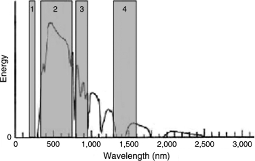
The four spectral ranges are:

– band from 200 nm to 280 nm or ultraviolet band or C-band;

– band from 350 nm to 750 nm or visible band (visible light communication — VLC);

– band from 800 nm to 950 nm or near-infrared band 1 (first window of fiber-optic communications and optical wireless);

– band from 1,300 nm to 1,600 nm or near-infrared band 2 or Telecom band (last window of fiber-optic and optical wireless communications).

Each band offers advantageous features and constraints consistent within the parameters outlined below:

– eye safety;

– optical disrupting;

– the optic link budget;

– ease of industrialization, that is to say, a low complexity;

– the transmitted power;

– the sensitivity;

– etc.

The choice of wavelength is therefore an important parameter in the realization of a wireless optical link.

We should also mention a few units used in the field of optical links:

– The amplitude of the electric field is measured in volts per meter (V/m).

– The amplitude of the magnetic field is measured in ampere per meter (A/m).

– The energy density of electromagnetic field is measured in watts per square meter (W/m²), or in milliwatts per square meter (mW/m²), or in milliwatts per square centimeter (mW/cm²).

Fundamentally, a wave is an oscillation, i.e. a periodic variation of a physical state that propagates in space or through matter. It is characterized by its amplitude, its direction of propagation, its speed, and its frequency in hertz.

The number of oscillations per unit of time is referred to as the frequency, and is measured in hertz (Hz).

The time interval between two successive oscillations with same direction and size is called the period. Its unit is the second (s).

The space traveled in by the wave during this time is the wavelength. Its unit is the meter (m).

The set of points reached by the disturbance in a homogeneous medium after a given time, starting from the time of emission, is referred to as the wave surface or wave front.

The relation among these different units (frequency, period, and wavelength) is presented below:

– The frequency f = 1/T.

- f = frequency in hertz (or multiple);

- T = period in seconds (or multiple).

– The wavelength = c × T = c/f.

- T = period in seconds (or multiple);

- c = velocity or speed of light = 3 × 10⁸ m/s or 299,792 km/s;

- f = frequency in hertz (or multiple).

– The period T = 1/f.

- T = period in seconds (or multiple);

- f = frequency in hertz (or multiple).

Depending on the field of study, different units are used for various spectral bands. Table 3.2 shows the relations among the frequency, the period, the wavelength, and the characteristics, depending on the part of the electromagnetic spectrum being considered. Different parameters are generally chosen merely for ease of use, but are associated with the same physical phenomenon.

However, it is recommended to use the international system MKSA (meter, kilogram, second, ampere) in calculations.

3.1.3.9. Examples of sources in the visible and near visible light

We now present a few examples of optical sources and provide some information concerning solar radiation. Indeed, it is important to know the spectral signature of these sources of perturbation for optical links since these radiations may disturb optical links in free space.

The main natural source of electromagnetic radiation is the Sun. Natural electromagnetic energy (solar radiation) allows, among other things, photosynthesis of trees and plants. Its spectrum extends from 300 nm to more than 1,500 nm, with varying intensities or amplitudes. The peak intensity is located approximately 480 nm (corresponding to the color blue) before progressively decreasing as the wavelength increases. Our eye perceives but a small fraction of solar radiation, that between 400 nm and 700 nm (see Figure 3.13). The Sun emits incoherent radiation. The Sun’s spectrum is shown in Figure 3.13 (for good visibility, the absorption peaks of oxygen molecules, ozone, and water are not shown) in intensity per unit frequency and MKSA unit is Wm⁻²Hz⁻1.

The Sun can be approximated as a black body. Another example of a black body is a filament lamp. The intensity of radiation from a black body at temperature T is given by Planck’s law of black body radiation:

For the Sun, this spectrum exhibits a maximum at the frequency f = 4 × 10¹⁴ Hz.

Another source of electromagnetic radiation, commonly used in both office and home environments, is the tungsten filament lamp.

Figure 3.14 shows the emission spectrum of a 60 W lamp. This spectrum is very broad and continuous, and exhibits a peak around 1,000 nm.

It might be stressed that optical communications use sources with a quasi-monochromatic narrow bandwidth (Figure 3.15) whose spectra can be compared instructively with the spectra resulting from ambient lights (the Sun, lamps, etc.). However, it is clear that for optical communication in free space, any source emitting in the spectral window of the detector is likely to disturb the transfer of information.

3.1.3.10. Conclusion

Since free-space telecommunication relies on the use of electromagnetic waves, it seemed essential to us to briefly describe some properties of these waves. Likewise, since geometrical optics is extensively employed for simulating free-space links, it was necessary to present the relation between electromagnetic waves and light rays, as well as the practical limitations of geometrical optics.

3.1.4. Models for data exchange

3.1.4.1. The OSI model

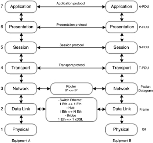
To describe the essential features for communication between computers in networks, the International Organization for Standardization (ISO), a dependent of the United Nation (UN) and made up of 140 national standards bodies, proposed a model called the Open Systems Interconnection (OSI) reference ISO 7498.

This model describes a particular reference level in network modeling. It consists of seven layers (see Figure 3.16):

– The physical layer transmits signals between equipment. The data are bits, for example RS232, xDSL, or WiFi.

– The data link layer manages communications or error-free transmissions of frames between two adjacent network equipment (MAC layer, such as ATM and Ethernet).

– The network layer manages communication step-by-step and provides the functions of addressing and routing packets (e.g. ARP and IPv6).

– The transport layer handles communications between end-to-end processes (running programs) and makes cutting or reassembly information (e.g. TCP and UDP).

– The session layer manages the synchronization of exchanges and allows opening or closing trading session (e.g. Real Time Streaming Protocol (RTSP) and Telnet).

– The presentation layer and code structure of data exchanged by applications (e.g. ASCII and Videotex).

– The application layer is the user access to network services via the application (e.g. HTTP, VoIP, and Mozilla).

Each level consists of the following:

– A service that provides primitives. These are commands, such as a connection request “connection.request”, or events, such as receiving data “data.indication”.

– A protocol that consists of a set of messages and rules for exchanges to achieve this service. The messages of a protocol are called protocol data unit (PDU). Some features of a protocol, such as the detection of transmission errors, the correction of these errors, and flow control, may be present in several levels.

– An interface that is defined as the access point to service in the standard. It is characterized by the library functions in a program, for example, or by a set of registers to the input of a circuit in a hardware configuration.

The process of data exchange between layers is generally similar. After a connection request from the applicant “connection-request”, the requested informs the demand “connection-indication” and responds either positively or negatively “connection-response”, which is validated by the applicant “connection-confirmation”. The latter event is an acknowledgment. Data transfer follows the same process (“DATA.request”, “DATA.indication”, and “DATA.confirm”) [TOU 03].

For example, to emit, the layer level N + 1 sends data to layer level N with the primitive “DATA.request”. These data will be encapsulated according to the protocol layer N + 1 (N + 1-PDU). In turn, the layer of level N will encapsulate the data according to its own protocol (N-PDU) before transmitting to N − 1. Upon receipt, each layer protocol analysis corresponding to its layer de-encapsulates the data and transmits them to the top layer with the primitive “DATA.indication”.

But the text of the standard is very abstract because there was the desire to make it applicable to virtually any network. As a result, a different model, simpler and more widely used, has emerged: the Transmission Control Protocol/Internet Protocol (TCP/IP) model (Figure 3.17).

3.1.4.2. The DoD model

The TCP/IP model was developed in the mid-1970s as part of the research DARPA (Defense Advanced Research Projects Agency, — the USA). This model should meet the needs of interconnects computer systems of the Army (Department of Defense — DoD).

It incorporates the modular approach, but it consists of four layers:

– The network layer includes the physical layer and data link layer of the OSI model. For example, Ethernet is a typical implementation of this layer because it can send and receive IP packets in a network.

– The Internet layer performs the interconnection of remote networks. It provides the functions of routing packets independently of each other until the final destination. The routing function allows us to compare it to the network layer of the OSI model. Its name is Internet Protocol (IP).

– The transport layer is the same as that of the OSI model. In this model, this layer has two implementations: TCP and User Datagram Protocol (UDP); it can transmit data faster but less reliable because there is no acknowledgment.

– The application layer, unlike the OSI model, is immediately above the transport layer and contains all higher level protocols such as Telnet, Trivial File Transfer Protocol (TFTP), Simple Mail Transfer Protocol (SMTP), and HyperText Transfer Protocol (HTTP).

3.2. Wireless optical communication

It was the U.S. Department of Defense (DoD) that was the first to recognize the value of optical wireless links because of their potential to provide links that could not be intercepted or interrupted. From 1944, the Navy tested an infrared military telephone. The phone operated with an infrared lamp using vapors of cesium (852 nm and 894 nm) for transmission and a photocell associated with an audio amplifier for reception.

Subsequently, by studying the main technological challenges of engineering related to these telecommunication systems, the activity of defense and aerospace engineering has helped establish a strong technical and scientific basis on which were based commercial optical communication systems.

Then, in the late 1990s with the advent of the Internet and the strong need for speed in the telecommunications sector, several companies have developed a new generation of outdoor optical communication systems for commercial use and adapted to the private sector. Then in the mid-2000s, faced wih the growing need for home or business use, and to deal with the various proposed radio solutions with the constraints of power and spectrum resource, indoor wireless optics communications solutions emerged as a relevant alternative.

3.2.1. Outdoor wireless optical communication

3.2.1.1. Earth-satellite wireless optical communication

The first known project was initiated in the 1970s [MAY 05]. It was called Spaceborne Flight Test System (Space Flight Test System) program and had the code number “405B Program”. It was at that time “the study of a space laser communication” in the Weapons System (WS) projects, funded entirely by the U.S. Air Force and the Pentagon. This project was conducted with the participation of NASA, DARPA, Goddard Space Flight Center, and Jet Propulsion Laboratory.

During the same period and always with the financing of the U.S. military, telecommunications links between aircraft have been tested using high-power lasers. Then, logically, these experiments were extended in the 2000s with programs such as Oracle or Orcle. These programs proposed wireless optical communications prototypes from ground–ground, ground–plane, plane–airplane, satellite, aircraft, and satellite–submarine or high-altitude platform communication [GIG 02, HAP 11, HEN 05, HOR 04] or drones [LOH 11].

Finally, around 2005, studies were conducted on communications between Earth and modules on Mars (NASA’s Space Exploration Initiative — SEI) with the Lewis Research Center Laboratory. It was to use lasers in order to achieve data rates of 100–1,000 Mbps. The findings of preliminary studies showed the availability of a complete system for 2020 [KWO 92].

3.2.1.2. Intersatellite wireless optical communication

In the 1990s, civil studies were initiated for intersatellite communications, and in November 2001, the first civilian application of laser high-speed communication was implemented. A 50 Mbps link was established between the French satellite SPOT-4 and the European satellite Artemis, separated from the other by tens of thousands of miles. Figure 3.18 represents a wireless optics communication between SPOT-4 satellite and Artemis satellite, by using the Silex laser system.

This European success is the result of a project called Semiconductor Intersatellite Link Experiment (SILEX) initiated in the early 1990s. The partners were Matra Marconi Space, Astrium, the European Space Agency (ESA), and the Centre National d’Études Spatiales (CNES).

Since 2008, the German Space Agency (DLR) operates an intersatellite link between the satellite TerraSAR-X and NFIRE. This connection is based on a second generation of laser communications technology. This solution will also be used for the new European satellite data relay (European Data Relay Satellite — EDRS) in 2013. The low power consumption and compact size have favored this approach over the radio.

3.2.1.3. Free-space optic

In France, the first trial of free-space laser communication was made in the late 1960s to Lannion between a building at the Centre National d’Études des Télécommunications (CNET) and trailer laboratory [TRE 67]. The device used a helium–neon laser of wavelength 632.8 nm at the emission side and a photomultiplier at the reception. Another study looked at a carbon dioxide laser wavelength of 10.6 µ. Video transmission tests were carried out over a distance of 1.2–19 km.

Other products, commercially mature, appeared in the world in the mid-1980s. But despite advances in technology, transmitters and sensors, transmission quality and availability of communication links did still not meet the expectations of a telecommunications operator.

But in the early 2000s, a new wave of products was proposed, mainly from European and American origin. These devices were tested by Centre Commun d’Études de Télévision et Télécommunications (CCETT) from Rennes (France) in order to determine what market segments the digital communications technology could propose.

The telecommunications market has become competitive; these technical solutions have been proposed as an extension to optical fiber or private Ethernet intersite communications.

The framework for using these wireless optical systems has been developed with the International Telecommunication Union (ITU) [ITU 11] and more specifically the ITU-R, CE3 [ITU 03, ITU 04, ITU 05b, ITU 07a, ITU 07b], CE5 [ITU 05a, ITU 08], and CE9.

3.2.2. Indoor wireless optical communication

The development of indoor wireless optics communication has existed since the early 1980s with a different approach to technical solutions according to the objectives, needs, and technological advances.

Table 3.3 outlines a non-exhaustive history of optical communications mentioning the company or the laboratory, the proposed data rate, the type of propagation, the modulation, and the used wavelength.

Wireless optical communications in limited space found many markets in domestic, transportation, and the office domain. Before dwelling on four typical examples, we can mention some everyday uses: wireless optical mouse and wireless keyboard, video game controllers with position sensing (indoor positioning — IdP), the wireless door key for access to homes or vehicles, the bar code reader and the electronic tag in the supermarket, and the wireless stereo headphones. There are also more innovative applications such as wireless optical communications between integrated circuits on a printed circuit board and the wireless optical network sensors in a plane [DAV 09].

3.2.2.1. The remote controller

By definition, a remote control is an electronic device for PtP unidirectional used to modify the remote operation of equipment, such as a TV channel and the volume. The first public television remote control appeared in 1955 (Zenith with Flash-Matic). It used visible light and four-cell reception (on/off, volume and the channels selection). One year later, wireless radio technology, with a greater coverage, replaced the light solution. But radio waves pass through obstacles such as walls, resulting in potentially changing the TV program in the neighborhood. The infrared solution was then finally retained.

Since the early 1980s, the vast majority of remote controls use infrared technology, and dispatch of orders is done by transmitting a digital signal, whose frequency is modulated at a few tens of kilohertz. Owing to the proliferation of owner controllable devices by a remote controller, up to 10 per household, there is now universal remote controller that controls all or part of the buttons. They are configurable or appear on an LCD touch screen.

3.2.2.2. The visible light communication

Visible Light Communication Consortium (VLCC) is a Japanese association, which aims to search, develop, and propose standardization of communication systems, using a ubiquitous solution, LED in the visible spectral range. Communication is achieved by intensity modulated at high frequency, with a consideration for human security. The use of communication is available in personal lighting, offices, car lights or road infrastructure (Intelligent Transport System — ITS), electronic signs for advertising, etc. The advantage of this approach is to offer a unique solution for lighting and communication. From 2007, papers were proposed and new working groups from the IEEE 802.15 [WON 07] have been created (IEEE 802.15.7) to provide communications solutions in the visible area with PtP and point-to-multipoint (PmP) solution.

3.2.2.3. The IrDA solutions

Another use case that comes from Infrared Data Association (IrDA) offers a 1 Gbps PtP solution called Giga-Ethernet (previously known as EFIR) for a distance of 0.2 m [KDD 11]. To meet the demands of rapid data transfer, the members of this association are intending to provide such a system in 2012. Examples of use are a portable multidevice interface and fast music or film download.

As part of a collaborative project called Regional Techimages, Orange Labs in Rennes, with regional research partners, have achieved a PtP at 1.25 Gbps over a distance of 0.5 m [BOU 09]. As part of a European collaborative project called Omega [OME 11a], the 1.25 Gbps data rate was achieved over a distance of 3 m.

3.2.2.4. The indoor wireless optical network (WON)

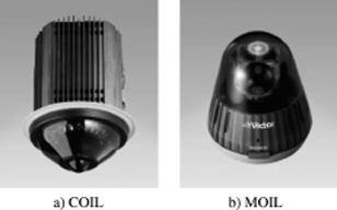
The VISPLAN product was the first system providing a wireless optical communication network, and it was only sold in Japan by JVC. VIPSLAN is typically a WLAN or a WDAN in direct competition with WiFi solutions. But the first version of WiFi pushed this device into the background. Based on the work of the Infrared Communication Systems Association (ICSA) [ICS 11] and the recommendations of the IR PHY IEEE 802.11 [IEE 11b], it offered a rate of 10 Mbps, then 100 Mbps.

The device (Figure 3.19) consisted of two elements:

– the base station (or COIL — Figure 3.19(a)) providing a data rate of 100 Mbps Ethernet with a range of 5 m (coverage of about 25 m²) in WLOS propagation;

– modules (or MOIL — Figure 3.19(b)) with the same characteristics of speed and range mentioned above, but constituted of an automatic pointing device.

So far, in this last area, the home or business wireless network WDAN and WLAN, commercial success was not to progress and several reasons can be advanced:

– A non-economically viable offer for a PtM optical link budget in a room.

– A non-available or inadequate network m layer (MAC layer).

– A broadband access point (xDSL or FTTH) or a connectivity insuring an inter-room link and using the power line communication (PLC) technique or fiber optic was not available.

– The concepts of energy savings or safety were less important.

However, over the past decade, the increase in throughput was highly significant and did not seem to have reached its asymptote. WiFi (IEEE 802.11) is a perfect example.

In wireless communication, the growing need for throughput can make indoor wireless optics technology a good alternative or complementary solution to the radio systems because of some interesting features:

– A high throughput (>1 Gbps) can be achieved, like radio system (e.g. system at 60 GHz).

– A spectral availability of more than 700,000 GHz, unregulated or taxed.

– The optical transmission is limited within a room, so they are naturally more secure.

– It is possible to reuse the same optical wavelength in the next room or the neighboring apartment with the same level of security.

– The installation of equipment is more intuitive (optical propagation).

– There is no suffered or performed interference with radio systems.

– The safety aspect or immunity refers to recognized international standards (IEC or FCC 60825).

3.2.3. The institutional and technical ecosystem

Communication solutions in wireless optical communications in limited space can be divided into several areas, shown in Figure 3.20.

– VLC: The application VLC was first devoted to PtP, short-range, and low data rate solutions by the VLCC association. But due to the work done within the IEEE 802.15.7 Working Group, VLC specification became wider.

– IEEE 802.15.7: IEEE 802.15 committee focuses on the development of PtP and PmP standards of WLAN in the visible area. In this context, a task group (TG) dedicated to the VLC was established in January 2009. Called 802.15.7 and chaired by Samsung, this working group has proposed a standard in 2010 whose main specifications are:

- the PtP and PmP solutions with a star or an ad hoc network configuration;

- two physical layers (PHY layer): Type 1 low data rate (10–100 Kbps) and Type 2 high speed (3.2–96 Mbps);

- the low data rate applications are mainly for road signs information (ITS), the dissemination of information in public or domestic places, indoor geolocation and advertising messages;

- the applications for high speed concern diffusion in public space or for household purposes (music, video, etc.) or the fast downloading for mobile devices (PDA, phone, etc.).

– ECMA: The VLC was also discussed at the ECMA in 2009. To this end, a white paper presented by the Lumilink company was proposed to the Technical Committee 47 (TC47) and a presentation to Samsung to promote the potential of visible light LED for near field communication.

– IrDA: Established in 1993, IrDA is an association that works in the infrared. In 1997, the association suggested a recommendation for a PtP economic digital infrared module (Infrared Communication — IRC). The IrDA device was present on many portable devices such as phones and laptops and also on devices such as printers and video cameras. Several standards have been developed and these provide the increased flow (data rate). The final specification, completed in 2010, offers an Ethernet communication up to 1 Gbps. The goal is to offer this standard on the same equipment with various applications: multi-interface mobile devices, music or video downloading from a Kiosk or at the rental store, promotion or advertising message, etc. Members are Casio, Finisar, Fuji, KDDI, Mitsubishi, NEC, NTT, Panasonic, Sony Ericsson, etc.

– OWMAC: The Optical Wireless Media Access Control (OWMAC) protocol specification is clearly defined for PmP broadband in a home or business network [OME 09]. This specification is wavelength independent and can more integrate the IEEE 802.15.7 and IrDA applications, and home automation applications.

If we have to make a comparison with another technological solution, it is always a very delicate operation as it should, initially, harmonize the above mentioned characteristics definitions.

In addition, it is preferable and realistic to better define the different radio and wireless optical technologies in a complementary than a competitive aspect.

However, a qualitative comparison (Table 3.4) is available from a radio technology that has similar characteristics (systems in 60 GHz) in order to obtain a more general view on the advantages and disadvantages of these two technologies.

Indoor wireless optics network is much less mature than radio systems, but it can be seen as having some equivalences, although it is difficult to make a comparison to “equivalent basis”.

Other parameters may be considered, such as energy use and safety. We now address the first aspect of the wireless optical communication, the transmission channel modeling.

Table 3.4. Comparison between 60 GHz radio and wireless optical technologies

Features	Radio 60 GHz	Wireless Optic
Spectrum availability	Reduced	Abundant
Spectrum regulation	Restricted	Free
Spectrum fee	Important to free	Free
Multipath fading	Very important	None
Data security	Encryption	Intrinsically secure by the walls
Intersymbol interference	Low	Potentially significant at high speed
Created or suffered electromagnetic interference	Possible if similar frequency or harmonic	None
Dominant noise	Other users	Artificial light and daylight
Human safety	Epidemiological study ongoing	Safety (Class 1) Internationally accepted standards