Chapter 5
Indicators of Price Levels
Prices of goods and services change. Sometimes the cause of the change is a temporary imbalance between supply and demand. When there is excess demand relative to supply, there is an upward pressure on the market price, and when supply exceeds demand there is a downward pressure on price. Since prices must be sufficiently high to cover costs for a business to sustain its operations, but not so high as to lose business to competitors, the price a firm will charge is affected by changes in the prices it must pay to acquire the labor, raw materials, energy, and other resources needed to provide its product or service. Consequently, price changes in one sector of the economy spill over to other sectors. Further, as we will discuss in chapter 9, macroeconomic policy can affect price levels. This chapter deals with economic indicators that monitor changes in prices.
Inflation
The economy is a largely closed system whereby the providers of resource inputs to one sector of the economy are also either directly or indirectly purchasers from the sectors to which they sell. As we saw in the previous two chapters, consumers are both the largest recipient group of final goods in GDP and the group receiving most of the income from the creation of final goods in the GDP. When the prices that consumers pay increase substantially, incomes must increase for consumers to be able to continue to acquire the goods and services they need. The increase in incomes, in turn, puts more cost pressure on the goods and services that require labor, resulting in a positive feedback loop. For this reason, prices for most goods and services tend to move in tandem.
When purchasers in an economy generally have to pay more to acquire the same physical goods and services, there is said to be price inflation. When the costs of acquiring the same physical goods and services decrease, there is said to be price deflation. The rate of inflation is usually expressed as the percent increase on an annualized basis. (In the case of deflation, the rate is usually expressed as a negative percent increase.)
We will discuss the role of inflation in macroeconomic policy in chapter 9, but here we can say that when the rate of price inflation is high and uncertain, inflation itself creates turmoil for the economy. In making decisions on capital investment and business strategy, most businesses need to anticipate the future prices they will receive for the goods and services they sell and how much they will pay for the goods and services they buy, even years in advance. When inflation is high and uncertain, projects that require investment of resources look very risky and firms may hold back from investment as a result. Also, when inflation is high and uncertain, both firms and employees will endeavor, if possible, to increase the prices for the goods and services they provide, not only to compensate for recent increases in prices they pay, but in anticipation of even higher costs they expect to face in the near future, thereby stirring more price inflation.
In this chapter, we will consider some important indicators of price levels that help determine the degree of price inflation present and whether inflation is increasing or decreasing. Initially, we will address some broad indicators that reflect general price level changes. Next, we will examine some indicators that track the prices of key goods or sectors of the economy.
The Consumer Price Index
Probably the most widely reported measure of general price levels in the United States is the Consumer Price Index, or CPI. The intent of the index is to provide a relative measure of prices faced by consumers in one time period compared to other time periods. Prices are weighted by amounts of each item that are used by a typical household, called a “market basket.” The index is prepared by the Bureau of Labor Statistics (BLS) in the U.S. Department of Labor, which reports new index values on a monthly basis. Reports are issued near the middle of the month following the month of the report.1
The BLS actually prepares two CPI indexes: The CPI-U tracks general price levels for urban consumers, which represents about 87% of the U.S. population. The CPI-W tracks price levels for wage earners, which represents about 32% of the population. Both indexes use the average prices over the three-year period from 1982 to 1984 as the base period values. Indexes are reported for four regions of the nation (northeast, midwest, south, and west) and several metropolitan areas.
Reports are usually cast in the form of percent increases from the prior month and percent increases from one year earlier. Values are reported with and without seasonal adjustments. Figure 5.1 shows the annual average CPI-U from 1970 to 2010. Figure 5.2 shows the year-to-year percent change in the CPI-U for the same period. The values in the second graph provide an estimate of inflation rates faced by urban consumers.
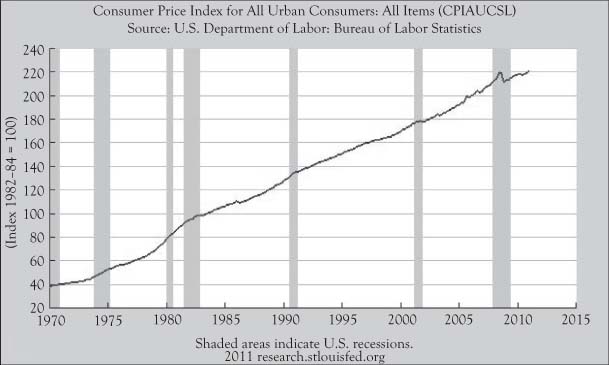
Figure 5.1. Consumer price index for urban consumers, all items, seasonally adjusted, from 1970 to 2010. (Source: Federal Reserve Bank of St. Louis, FRED Economic Data.)

Figure 5.2. Percentage change from one year earlier in consumer price index for urban consumers, all items, seasonally adjusted, from 1970 to 2010. (Source: Federal Reserve Bank of St. Louis, FRED Economic Data.)
The composition of the market basket is determined from the Consumer Expenditure Survey. This composition changes over time due to changes in what consumers buy. For example, over the last century, consumers have changed from eating relatively higher amounts of pork, to relatively higher amounts of beef, and later to relatively higher amounts of chicken.
The monthly reports also provide indexes for prices of the individual items in the market basket, as well as the percent month-to-month and 12-month changes in the prices of those items. Prices of some of these components are more volatile than others. Items related to food and energy tend to fluctuate more due to the random effects of weather on food and the impact of political events on foreign supplies of crude oil. The CPI measures are reported with food and energy items excluded to form what is called a core CPI. This measure is more stable and often cited as a better indicator of inflation in consumer prices.
The percentage change in the CPI is sometimes used to estimate changes in the cost of living. Many programs, including federal government programs like Social Security, use the CPI-U as the basis for adjusted payments from year to year. The CPI-U is also the basis for adjusting income brackets for individual U.S. income taxes.
However, the BLS states that CPI is probably an upper bound for the change in the cost of living, because it does not account for consumer decisions to substitute consumption in response to price changes so as to get more utility per dollar of expenditure. The BLS has started reporting a Chained CPI-U that better accounts for this substitution.2
During the last century, the CPI was criticized for not reflecting quality changes in a commodity. For example, a television set purchased in 2011 has different features and quality than a television purchased in 1982. In some cases, items are no longer sold and have been replaced with similar, but not identical items. The BLS has developed a technique called a hedonic quality adjustment to try to address this issue and has been expanding the use of this adjustment to a wider array of goods and services.3
The PCE Price Index
The Bureau of Economic Analysis, in conjunction with its data collection, analysis, and reporting of personal income and outlays, provides another index of inflation in consumer prices. Since this index is based on expenditures on the items included in the personal consumption expenditures component of GDP, it is known as the PCE Price Index. Like personal income and outlays, it reports the index on a seasonally adjusted monthly basis, with 2005 as the base year. However, the new value is usually expressed in terms of the annualized percent increase from the prior month. The monthly percentage change in the index excluding food and energy is announced as well.
The PCE price index appears to be measuring changes in same set of consumer prices as the CPI. In fact, in preparing the PCE, the BEA uses data from the Bureau of Labor Statistics, which produces the CPI. Month-to-month changes in the PCE price index are often close to the CPI-U, as shown in Figure 5.3 for years from 1970 to 2010. One reason for any difference is that while the CPI is based on prices paid directly by consumers, the PCE price index includes expenditures by nonprofit organizations on behalf of individuals. Another source of difference is that the weights assigned to components in the PCE price index change from month to month to reflect changes in purchasing patterns, while the CPI only revises the expenditure weights every two years. (However, the methodology used in calculating Chained CPI-U does reflect period-to-period changes in purchasing patterns.)
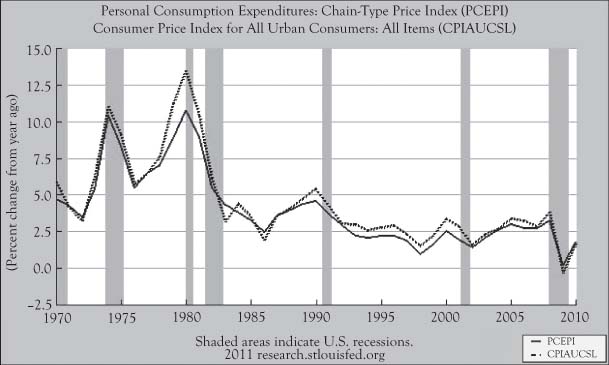
Figure 5.3. Percentage change in annual PCE price index vs. CPI-U, seasonally adjusted, from 1970 to 2010. (Source: Federal Reserve Bank of St. Louis, FRED Economic Data.)
The PCE price index has received increased attention due to a belief that the Federal Reserve places greater trust in the PCE index than the CPI-U as an indicator of inflation. Analysts and investors who are trying to guess how the Federal Reserve will act in its next meeting use the PCE price index reports as a basis for those guesses.
The Producer Price Index
The CPI and PCE price indexes focus on final goods that are directed at consumers. While prices for other goods and services in the economy mirror the general movement in consumer prices, there are differences in timing and magnitude. Since consumer price changes are driven by changes in production costs, price changes may occur first in basic materials and intermediate goods before being manifested in final consumer goods. Some firms have “pricing power” that allows them to pass along cost increases in the form of higher prices, even in a weak economy, without suffering a significant loss in sales volume. However, in times when the consumer demand is soft, it is possible for prices of some basic materials and intermediate goods to rise without being passed along a price increase to the consumer.
To track prices across the economy at all stages of production, the Bureau of Labor Statistics compiles a monthly Producer Price Index (PPI).4 The index is built from individual price indexes for thousands of goods and services, with recent values of the index and month-to-month changes of each in the detailed monthly report. The BLS uses 1982 as the base year for prices, but updates quantity weights every five years to reflect changes in the economy. The report is issued near the middle of the month following the month featured in the report.
In addition to providing a total producer price index, goods are classified as being finished, intermediate, or crude. Finished goods are goods for which processing is complete and are ready for distribution or sale. An example would be an automobile that has completed assembly. Intermediate goods are those where some processing is complete, but there is additional processing to go. A manufactured part that has no value as a good in itself, like a dashboard for a car, would be an intermediate good. Crude goods are goods that have been extracted via farming, forestry, or mining, but not processed.
Figure 5.4 shows the PPI components for finished goods and crude goods on the same graph from 1970 to 2010. Clearly there is more fluctuation in the price index for crude goods than finished goods, with the spikes corresponding to periods when there were spikes in oil prices. Crude goods are based more on commodity prices and less on labor costs than finished goods.

Figure 5.4. Producer price index for fi nished goods and crude goods, seasonally adjusted, from 1970 to 2010. (Source: Federal Reserve Bank of St. Louis, FRED Economic Data.)
The monthly report provides individual producer price indexes for 15 major sectors of the economy. The portions of the PPI related to food and energy are reported separately, and those components are extracted from the total PPI to provide a core PPI. As with the CPI and PCE Price Index, the lead report on the PPI is expressed in terms of percent change from the prior month and seasonally adjusted. Also, since the PPI tracks prices of individual items and those items are periodically replaced or updated with similar items of different functionality, the BLS makes quality adjustments to some item indexes.
A graph showing year-to-year percent change in the PPI from 1970 to 2010, compared to the CPI, appears in Figure 5.5. Note that the changes in the CPI largely track the changes in the PPI, though not exactly. Again, there are good reasons to expect the indexes to track closely: consumer prices are related to the costs of producing consumer goods and many of the finished goods in the PPI are intended for personal consumption. The PPI sometimes moves slightly in advance of the CPI, particularly when the CPI is compared to the PPI indexes for crude or intermediate goods.
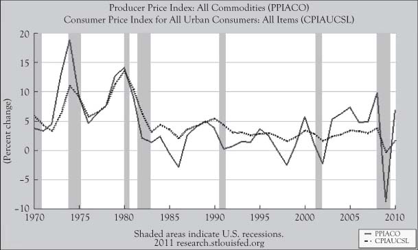
Figure 5.5. Average annual percent change in PPI and CPI-U, seasonally adjusted, from 1970 to 2010. (Source: Federal Reserve Bank of St. Louis, FRED Economic Data.)
The GDP Deflator
The data collected by the Bureau of Economic Analysis to calculate the PCE price index is part of a broader ongoing project to collect data on prices of all final goods in the U.S. domestic economy. These efforts are necessary to be able to express GDP and GDP components in terms of real dollars (currently with 2005 as the base year.) The basis for converting GDP to a real dollar amount uses a chained price index that, as with the index used in the PCE price index, better responds to substitution than price indexes like the CPI and PPI, which use fixed quantity weights to aggregate the price changes of individual items into a single index.
The ratio of the GDP in nominal (or current) dollars in a period to the associated real dollar value in that period creates an index-like measurement called the GDP deflator. By examining changes in the deflator from one quarter to the next and then annualizing the change, one gets an estimate of the inflation rate for all final goods in the economy.
Although the GDP deflator reflects price changes over a wider range of final goods, the deflator closely tracks the PCE price index. Since the PCE price index is estimated on a monthly basis and the GDP deflator is estimated quarterly, the PCE price index tends to receive more attention in the business media.
Average Hourly Earnings
Labor is generally a dominant expense for businesses, and wages and salaries are the main source of income for most households. If wages outpace consumer prices, households can either increase savings or increase consumption. If consumer prices outpace wages, consumers will either reduce savings or consumption. The wages and salaries received by an individual are the product of the number of hours worked and the rate of earnings per hour. We will examine an indicator of the number of hours worked in chapter 7. For a typical person fully employed at 40 hours per week, change in earnings per hour reflect changes in that person’s income from wages and salaries.
The Bureau of Labor Statistics releases a report called The Employment Situation in the early part of each month.5 One item in that report is the average hourly earnings of employees on nonfarm payrolls in the previous month. While not a formal index, it can be used as an index of the average earnings corresponding to an hour of employed labor. The report states the change in earnings per hour in monetary amount and percent change.
The BLS started reporting average hourly earnings of all employees on nonfarm payrolls in 2006. This indicator expands the base of employees represented in another monthly BLS time series that measures average earnings of production and nonsupervisory employees of private businesses. Interestingly, average hourly earnings for production and nonsupervisory employees in private businesses have climbed at a fairly steady rate over the last 30 years. The increase continued even during periods of recession, when unemployment increased, and there was an excess supply of labor.
The Employment Cost Index
From the perspective of employers, compensation of employees is wages and salaries plus benefits. The Bureau of Labor Statistics prepares a quarterly employment cost index to track these components.6 The index uses 2005 for a base year and is seasonally adjusted. The report appears at the end of the month following the end of the quarter.
The report also separates the employment cost index into a wage and salary index and a benefits index. A graph of these separate indexes from 2001 to 2010 appears in Figure 5.6. Note that the cost of benefits rose faster than wages in the first five years.
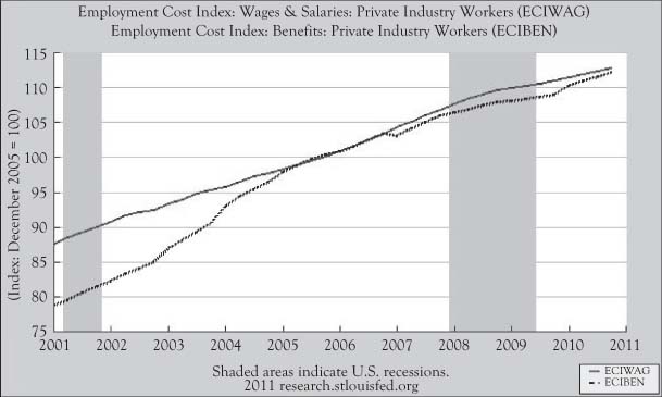
Figure 5.6. U.S. Employment cost index for wages and salaries and employment cost index for benefi ts, private industry workers, seasonally adjusted, from 2001 to 2010. (Source: Federal Reserve Bank of St. Louis, FRED Economic Data.)
The detailed report provides separate employment cost indexes for employees in private firms and employees of government. There are also separate indexes for major private sectors.
The S&P/Case-Shiller Home Price Indices
In studying changes in home prices, economist Karl Case developed a method for estimating the rise in home prices looking at repeat sales of homes. Based on an impression that the rise in home prices was not sustainable, he worked with economist Robert Shiller, and the two concluded there was a housing market “bubble” prior to the collapse of residential real estate prices in the first decade of this century.
Case and Shiller expanded their research into an ongoing program based on a modification of their repeat sales methodology with monthly reports that are published by Standard & Poors.7 Data are collected from 20 metropolitan areas. In addition to price indices for each area, there is a 20-city composite index that uses 2000 as the base year. Cities are weighted by the relative value of real estate in each metropolitan area. The composite index for 20 cities begins in the year 2000. Originally data were collected in 10 of the metropolitan areas. There is a composite index reported for these 10 areas that dates back to 1987.
While the index and changes in the index are reported monthly, the index is actually based on a three-month moving average of repeat sales data. The indices are published on the final Tuesday of the second month following the month featured in the report. Houses that undergo substantial change after the initial purchase are excluded to avoid problems with changes in quality. The analysts also remove repeat sales that do not involve two sales that are both arm’s length exchanges between private parties.8
Sales Price of Existing Home Sales
The National Association of Realtors maintains a considerable database of existing homes that sold or are available for sale. This organization offers a public report toward the end of every month summarizing sales of existing homes and pending home sales.9 Sales are reported for different regions of the country (northeast, midwest, south, and west). Single-family homes and condominiums are reported separately. Sales prices are reported by median price and average price.
While the S&P/Case-Shiller report provides a reliable guide for the rate of change in home prices by its focus on repeat sales, the report from the National Association of Realtors provides a readily understandable measure in terms of the typical price.
The report also includes counts of the home sales, both seasonally adjusted and not adjusted. While existing home sales do not involve the same level of production activity as a new home, an increase in sales does portend additional economic activity in terms of renovation work and new appliances. As a major capital expense, an increase or decrease in home sales also serves as an indicator of consumer confidence.
The inventory of unsold homes-for-sale is identified and expressed in terms of the number of months of supply at the expected rate at which houses will sell. In the aftermath of the bust in home prices and rise in mortgage defaults, there has been over 12 months of supply of existing homes.
Price of New Houses Sold
The Bureau of the Census compiles data on new home sales similar to what the National Association of Realtors provides for existing home sales. A report is issued monthly, usually shortly after the National Association of Realtors’ report.10 The figures are subject to revisions in subsequent monthly reports.
Figure 5.7 shows the median price of new houses sold in the United States from 1963 to 2010. Note that during most recessions (indicated by the darker bands), median housing price increases stalled, but did not decrease much. However, in the recession that began in 2007–08, the median price of new homes sold dropped around 20%, and has only increased slowly.

Figure 5.7. Median price of new houses sold in the U.S., monthly and not seasonally adjusted, from 1963 to 2010. (Source: Federal Reserve Bank of St. Louis, FRED Economic Data.)
In addition to the median and average prices, the report provides a distribution of how many new homes sold in various price ranges. The report includes counts of homes sold, seasonally adjusted and not adjusted, the median time a sold new home was on the market, and the number of new homes for sale at the end of the reporting period.
In chapter 2 we discussed the presence of random fluctuations in time series. We cautioned that the magnitude of these fluctuations can sometimes be large enough to lead to a wrong conclusion about the direction in which an indicator is moving. This caution is particularly pertinent in looking at a single month-to-month change in any of the indicators for housing prices in the last three sections, particularly when applied to individual metropolitan or county markets. The National Association of Realtors has local affiliates that prepare the same indicators for existing home sales in their territory as the national parent does for the nation. Due to the relatively small number of sales in these territories, there can be considerable random fluctuation, even in the median selling price.
Oil Price
In the 1970s, the United States learned painfully how dependent it had become on petroleum. Despite the fact that the world oil industry started in the United States, by the 1970s the amount of the petroleum drilled domestically became substantially less than the amount consumed domestically. As the result of the exercise of market power by countries that exported oil and political problems in the Middle East, the price of crude oil jumped dramatically after a long stable period when crude oil had remained about $3 a barrel. Oil ratcheted first to prices above $10 and then to almost $40 by 1980. The price per barrel dropped and remained around $20 for remainder of the last century. However, with the emergence of industrial economies in China, India, and other developing countries, strong demand and political events have driven crude oil prices as high as almost $140 a barrel.
Jumps in the price of oil have a disruptive effect on the U.S. economy. The increase in the 1970s helped fuel strong inflation. The high price of crude oil translated to dramatic price increases in gasoline, which affected consumers by leaving reduced amounts for expenditures on other items. Consumers showed a greater tendency for smaller cars that were more fuel efficient, which opened the U.S. door to foreign automobile manufacturers. The crude oil price increase in the last decade has brought a change in consumer preferences for hybrid and electric vehicles.
Oil price and gasoline price data are widely available on the Internet. One public source of price data is the Energy Information Administration (EIA) of the U.S. Department of Energy.11 The EIA provides prices of crude oil on a daily, weekly, monthly, quarterly, and annual basis.
Crude oil prices vary considerably depending on the quality of the oil and where it is drilled and delivered. One popular reference price is the spot price of West Texas Intermediate (WTI) light sweet crude oil delivered to Cushing, Oklahoma and exchanged on the New York Mercantile Exchange. A second popular reference price is the spot price of Brent European North Sea crude oil. These two spot prices tend to move in tandem, but sometimes there are discrepancies caused by excess supplies. Both prices are reported by the EIA and other financial websites and media.
Agricultural Prices
One of the oldest programs in data collection in the United States is in the study of its agricultural sector. While the United States became the largest industrial economy in the world during the twentieth century, the country expanded geographically in the nineteenth century, and agriculture was usually the first major means of livelihood in newly settled territories. Most working Americans at the time were farmers and ranchers. When small farmers began to struggle in the early twentieth century as the result of intense competition and risk from climate, price support programs were created to stabilize the farming economy, supported by a substantial data collection operation by the U.S. Department of Agriculture.
The National Agriculture Statistics Service (NASS) issues a report near the conclusion of every month that reports on agricultural prices in that month.12 The report lists prices received for a wide range of crops and livestock, as well as prices paid by farmers for resources. Collective indexes for prices received and prices paid are provided as well, currently using the three-year period of 1990–1992 as the base period.
The prices received index is considered a leading indicator of food-related items in the PPI and CPI. Fuel is a significant input to crop production, so dramatic changes in fuel costs will drive changes in crop prices received. Livestock operations use crops as a feed source, so a price jump in major feed crops like corn will usually result in a price jump for livestock like hogs, cattle, and chickens. In recent decades, corn has been harvested for the production of ethanol, encouraged by government subsidies. This additional consumption has created excess demand for corn, which in turn has driven food prices higher.