Chapter 5
Propagation in the Atmosphere
“Look at the light and consider its beauty.
Closes and opens the eyes quickly:
what you see is already passed
and what you saw is gone
Leonardo da Vinci,
Codex Forster,
1493–1505
5.1. Introduction
Laser beams, used to operate free-space optical (FSO) links, involve the transmission of an optical signal (visible or infrared) in the atmosphere. They interact with various components (molecules, aerosols, etc.) of the propagation medium. This interaction is at the origin of many phenomena such as absorption, diffusion, refraction, and scintillation. The only limitation known is heavy fog and they cannot cover distances more than a few kilometers. They are therefore suitable for the construction of networks between nearby buildings. The laser beams generally used have low power; and the environmental impact is negligible.
One of the challenges to take up is a better understanding of atmospheric effects on propagation in this frequency spectrum, to better optimize wireless broadband communications systems, and to evaluate their performance. It is a prerequisite to test communication equipments.
Atmospheric effects on propagation, such as absorption and molecular and aerosol diffusion, scintillation due to the change in the air index under the effect of temperature variation, hydrometeors attenuation (rain, snow), and their different models (Kruse and Kim, Bataille, Al Naboulsi, Carbonneau, etc.) are presented and confronted against experimental results.
The runway visual range (RVR), a parameter for characterizing the transparency of the atmosphere, is defined and various measuring instruments such as transmissometer and scatterometer are described.
5.2. The atmosphere
In the context of FSO links, the propagation medium is the Earth’s atmosphere. It may be regarded as a series of concentric gaseous layers around the Earth. From 0 to approximately 80–90 km in altitude, we have the homosphere and, extending beyond these altitudes, the heterosphere. When considering the temperature gradients as a function of the altitude, homosphere can be seen with three layers: the troposphere, the stratosphere, and the mesosphere.
In the case of FSO communications, the focus is particularly on the troposphere because most of the meteorological phenomena occur in this layer. The propagation of light in this layer is influenced by:
– the gaseous atmospheric mixing;
– the presence of small suspended particles of various sizes (0.1–100 µm), the aerosols;
– the hydrometeors (rain, snow, and hail);
– the lithometeors (dust, smoke, and sand);
– the changes in the gradient of air refractive index (propagation medium) which is at the origin of scintillation and turbulence.
5.2.1. The atmospheric gaseous composition
To characterize the properties of atmospheric transmission affecting optronic systems, the atmospheric gaseous components are classified into two categories: the fixed density and the variable density proportion components.
The fixed density proportion components (variation less than 1%) are the majority components. They have a quasi-uniform distribution for altitudes ranging between 15 km and 20 km. These include, for example, O2, N2, Ar, and CO2. In the visible and infrared wavelengths range up to 15 µm, CO2 gases give the only important absorption lines.
The variable density components are the minority and their concentration depends on the geographical location (latitude and altitude), the environment (continental or maritime), and the weather conditions.
Water vapor is the main component of the atmosphere. Its concentration depends on climatic and meteorological parameters. For example, in marine areas, its concentration can reach 2%, while above 20 km altitude its presence is negligible.
The water vapor concentration is determined from the atmospheric humidity and can be defined in three different ways:
– Absolute humidity (g/m3): the mass of water vapor per unit air volume.
– Relative humidity (%): the ratio between the absolute humidity and the maximum quantity of water vapor that could be contained in the air at the same temperature and at the same pressure.
– Number of mm of precipitable water (w0) per unit distance, usually per km.
Another major variable component is ozone (O3) whose concentration also varies with altitude (maximum content at 25 km), latitude, and season. It presents an important absorption in the ultraviolet and infrared radiation.
5.2.2. Aerosols
Aerosols are extremely fine solid or liquid particles, suspended in the atmosphere and with a very low fall speed. Their size generally lies between 0.01 μm and 100 μm. Owing to the action of Earth’s gravity, the biggest particles (r > 0.2 μm) are in the vicinity of the ground. Fog and mist are liquid aerosols, and salt crystals and sand grains are solid aerosols.
These aerosols may induce severe disturbances in the propagation of optical waves since their dimensions are close to the wavelength. This is not the case for the millimeter (EHF waves), decimeter (SHF waves), meter (UHF waves), and decameter (HF waves) radio waves.
5.3. The propagation of light in the atmosphere
The characteristic performance of FSO links for data transmission depends on the environment, the atmosphere in which they propagate. The atmosphere, due to its composition, interacts with the light beam (optical or infrared): absorption and molecular and aerosol scattering (fog, hydrometeors — rain, snow) and scintillation due to the variation of the air index as a result of temperature variations.
Atmospheric attenuation results from an additive effect of absorption and scattering of the infrared light by gas molecules and aerosols present in the atmosphere. It is described by Beer’s law, giving the transmittance as a function of distance:
where
– ![]() (d) is the transmittance at a distance d from the emitter.
(d) is the transmittance at a distance d from the emitter.
– P(d) is the signal power at a distance d from the transmitter.
– P(0) is the transmitted power.
– ![]() is the attenuation or the extinction coefficient per unit of length.
is the attenuation or the extinction coefficient per unit of length.
Attenuation is related to transmittance by the following expression:
Equation 5.2. Extinction coefficient
The extinction coefficient is the sum of four terms:
where
– ![]() m is the molecular absorption coefficient (N2, O2, H2, H2O, CO2, O3, etc.), note that this refers to the structure and the composition of the atmosphere.
m is the molecular absorption coefficient (N2, O2, H2, H2O, CO2, O3, etc.), note that this refers to the structure and the composition of the atmosphere.
– ![]() n is the absorption coefficient of the aerosols (fine solid or liquid particles) present in the atmosphere (ice, dust, smoke, etc.).
n is the absorption coefficient of the aerosols (fine solid or liquid particles) present in the atmosphere (ice, dust, smoke, etc.).
– ![]() m is the Rayleigh scattering coefficient resulting from the interaction of light with particles of size smaller than the wavelength.
m is the Rayleigh scattering coefficient resulting from the interaction of light with particles of size smaller than the wavelength.
– ![]() n is the Mie scattering coefficient; it appears when the incident particles are of the same order of magnitude as the wavelength of the transmitted wave.
n is the Mie scattering coefficient; it appears when the incident particles are of the same order of magnitude as the wavelength of the transmitted wave.
Absorption dominates in the infrared whereas scattering dominates in the visible and ultraviolet regions.
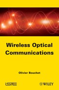
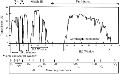
5.3.1. Molecular absorption
Molecular absorption is resulting from an interaction between radiation, atoms, and molecules of the medium (N2, O2, H2, H2O, CO2, O3, Ar, etc.). It defines different transmission windows in visible and infrared frequencies domain (Figure 5.1).
Figure 5.1. Transmittance of the atmosphere due to molecular absorption
5.3.2. Molecular scattering
It results from the interaction of light with atmospheric particles whose sizes are smaller than the wavelength. An approximate value of ![]() m (
m (![]() ) is given by the following relations:
) is given by the following relations:
Equation 5.3. Molecular scattering coefficient
with
where
– P(mbar) is the atmospheric pressure and P0 = 1,013 mbar.
– T(K) is the atmospheric temperature and T0 = 273.15 K.
As a result, scattering is negligible at infrared wavelengths. Rayleigh scattering primarily affects ultraviolet wavelengths up to visible wavelength. The blue color of the clear-sky background is due to this type of scattering.
5.3.3. Aerosol absorption
It results from the interaction between the radiated power and the aerosols, tiny particles suspended in the atmosphere (ice, dust, smoke, fog, and mist).
The absorption coefficient ![]() n is given by the following equation:
n is given by the following equation:
Equation 5.4. Molecular absorption coefficient
where
– ![]() n(A) is the absorption coefficient due to aerosols (km−1).
n(A) is the absorption coefficient due to aerosols (km−1).
– ![]() is the wavelength (µm).
is the wavelength (µm).
– dN(r)/dr is the particle size distribution per unit of volume (cm−4).
– n'' is the imaginary part of the refractive index n of the considered aerosol.
– r is the radius of the particles (cm).
– Qa(2![]() r/
r/![]() , n'') is the absorption cross section for a given type of aerosol.
, n'') is the absorption cross section for a given type of aerosol.
Mie theory [MIE 08] predicts the electromagnetic field diffracted by homogeneous spherical particles. It assesses both physical quantities, such as the absorption normalized cross section Qa and the scattering normalized cross section Qd. They depend on the particle size, refractive index, and incident wavelength. They represent the section of an incident wave normalized by the geometric section of the particle (![]() r2), such as the power absorbed (scattered) is equal to the power crossing this section.
r2), such as the power absorbed (scattered) is equal to the power crossing this section.
The refractive index of aerosols depends on their chemical composition. It is a complex number and depends on the wavelength. It is noted n = n′+ n″, where n′ is a function of the scattering capacity of the particle and n″, is a function of the absorption of the same molecule.
Note that in the visible and near-infrared spectral region, the imaginary part of the refractive index is extremely low and can be neglected in the calculation of the global attenuation (extinction). In the far-infrared case, the imaginary part of the refractive index must be taken into account.
5.3.4. Aerosol scattering
It results from the interaction of light with particles (aerosols, hydrometeors) whose size is of the same order of magnitude as the wavelength.
The scattering coefficient ![]() n is given by the following equation:
n is given by the following equation:
Equation 5.5. Aerosolar scattering coefficient
where
– ![]() n(
n(![]() ) is the scattering coefficient due to aerosols (km–1).
) is the scattering coefficient due to aerosols (km–1).
– ![]() is the wavelength (µm).
is the wavelength (µm).
– dN(r)/dr is the particle size distribution per unit of volume (cm−4).
– n' is the real part of the refractive index n of the considered aerosol.
– r is the radius of the particles (cm).
– Qd (2![]() r/k)
r/k)![]() , n') is the scattering cross section for a given type of aerosol.
, n') is the scattering cross section for a given type of aerosol.
The distribution of particle size is generally represented by an analytic function, such as the log-normal distribution for aerosols and the modified Gamma distribution for fog [BAT 92, KIM 01, KRU 62, NAB 04]. The latter is largely used to model different types of fog and clouds. It is given by the following equation [DEI 69, SHE 79]:
Equation 5.6. Distribution of particle size
where
– N(r) is the number of particles per unit volume whose radius ranges from r to r + dr,
– ![]() , a, and b are the parameters that characterize the distribution of particle sizes.
, a, and b are the parameters that characterize the distribution of particle sizes.
Software of atmospheric transmission calculations such as FASCOD, LOWTRAN, and MODTRAN considers two particular types of fog: the dense advection and the convection or moderate radiation which are modeled by the modified Gamma sizes distribution. Typical parameters are given in Table 5.1 [CLA 81, SHE 89].
Mie theory predicts the diffusion coefficient Qd due to aerosols. It is calculated assuming that the particles are spherical and sufficiently distant from each other so that the scattered field by a particle and arriving on another particle can be calculated assuming far-field regime.
Table 5.1. Parameters characterizing the particles size distribution
Notes:
– N is the total number of water particles per unit volume (nb/cm3).
– rm is the modal radius (µm) for which the distribution presents a maximum.
– W is the liquid water content (g/m3).
– V is the visibility associated to the fog type (m).
The scattering cross section Qd is a function that strongly depends on the size of the aerosol compared to the wavelength. It reaches its maximum value (3.8) when the radius of the particle is equal to the wavelength: the scattering is then maximal. As the particle size increases, it stabilizes around a value equal to 2. We must therefore expect a very selective function by the particles whose radius is less than or equal to the wavelength. Clearly, scattering depends strongly on the wavelength.
Aerosol concentration, composition, and size distribution vary temporally and spatially; it is difficult to predict attenuation by these aerosols. Although their concentration is closely related to optical visibility, there is no unique particle size distribution for a given visibility. Visibility characterizes the transparency of the atmosphere as estimated by a human observer. It is measured by the RVR. The scattering coefficient is the most detrimental factor in terms of FSO wave propagation.
5.4. Models
Different models of attenuation exist in the literature: Kruse and Kim, Bataille, and Al Naboulsi models; rain and snow attenuations; and scintillations.
5.4.1. Kruse and Kim models
The attenuation coefficient for visible and near-infrared waves up to 2.4 μm is approximated by the following equation:
Equation 5.7. Kruse and Kim model
where
– V is the visibility (km).
– ![]() nm is the wavelength (nm).
nm is the wavelength (nm).
The q coefficient characterizes the size particles. It is given by the following relation [KRU 62]:
As a result, attenuation is a decreasing function of the wavelength.
Recent studies have led to define the parameter q as follows [KIM 01]:
where V is the visibility (km).
As a result, attenuation is a decreasing function of the wavelength when visibility exceeds 500 m. For lower visibilities, the atmospheric attenuation is independent of the wavelength.
5.4.2. Bataille’s model
Bataille’s model [BAT 92] calculates the molecular and aerosol extinction for six laser lines (0.83, 1.06, 133, 1.54, 3.82, and 10.591 gm) by a polynomial approach on terrestrial links close to the ground. They are examined below.
5.4.2.1. Molecular extinction
The specific extinction coefficient ![]() m is obtained by a 10-term expression:
m is obtained by a 10-term expression:
where
– T' = T(K)/273.15 is the reduced air temperature.
– H is the absolute humidity (g/m3).
The coefficients Bi (i = 1.10) for different studied wavelengths are given in the literature [BAT 92] and [GEB 04].
5.4.2.2. Aerosol extinction
The specific extinction coefficient ![]() n is obtained by a 10-term expression:
n is obtained by a 10-term expression:
where
– V is the visibility (km).
– H is the absolute humidity (g/m3).
– x, y, and z are real numbers used to optimize the polynomial for each studied wavelength; their values are adjusted when the maximum relative error between FASCOD and the polynomial is lower than 5%. The coefficients Ai (i = 1.10) for the different studied wavelengths are given in the literature [BAT 92, COJ 99] for both types of aerosol: rural and maritime.
5.4.3. Al Naboulsi’s model
Al Naboulsi et al. [NAB 04] have developed simple relations from FASCOD enabling the attenuation in the range of wavelengths from 690 nm to 1,550 nm and visibility ranging from 50 m to 1,000 m for two types of fog: advection and convection.
Advection fog occurs when warm moist air moves over a cold floor. The air in contact with the ground cools and reaches its dew point, water vapor condenses. This type of fog occurs more particularly in spring when warm moist air moves from the south over cold regions. Attenuation by an advection fog is expressed by the following equation:
Equation 5.8. Attenuation by an advection fog
where
– ![]() is the wavelength (µm).
is the wavelength (µm).
– V is the visibility (km).
The radiation or convection fog is generated by the radiative cooling of an air mass due to the nocturnal radiation from the ground when meteorological conditions (very weak winds, high humidity, clear air, etc.) are favorable. Soil loses its heat accumulated during the day. It becomes cold. On contact, the air cools, reaches its dew point, and the humidity it contains condenses. We have the formation of a cloud close to the ground. This type of fog occurs most commonly in valleys. Attenuation by a convection fog is expressed by the following equation:
Equation 5.9. Attenuation by a convection fog
where
– ![]() is the wavelength (µm).
is the wavelength (µm).
– V is the visibility (km).
5.4.4. Rain attenuation
Rain is formed from water vapor contained in the atmosphere. It consists of water droplets whose form and number vary in time and spatially. Their form depends on their size: they may be regarded as spheres until a radius of 1 mm and beyond as oblate spheroid: ellipsoid generated by the revolution of an ellipse around its minor axis. The equivalent radius is generally introduced, the radius of the sphere that has the same volume.
The rain attenuation (dB/km) is generally given by the Carbonneau’s relation [CAR 98]:
Figure 5.2 shows the variations of the specific attenuation (dB/m) due to rainfall in the optical and infrared spectrum.
Figure 5.2. Specific attenuation (dB/km) due to the rain
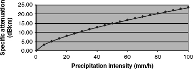
Recommendation ITU-R P.837 gives the rain intensity Rp, exceeded for a given percentage of the average year p, and for any location [ITU 04].
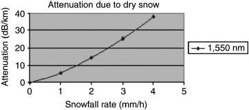
5.4.5. Snow attenuation
Specific attenuation due to snow as a function of snowfall rate is given by the following equation:
Equation 5.11. Attenuation due to snow
where
– Attsnow is the specific attenuation due to snow (dB/km).
– S is the snowfall rate (mm/h).
– a and b are functions of the wavelength (nm). They are given in Table 5.2.
Table 5.2. Parameters “a” and “b” for wet and dry snow
| a | b | |
| Wet snow | 0.0001023 |
0.72 |
| Dry snow | 0.0000542 |
1.38 |
The wet and dry snow attenuations as a function of snowfall rate for ![]() = 1,550 nm are given in Figures 5.3 and 5.4.
= 1,550 nm are given in Figures 5.3 and 5.4.
Figure 5.3. Wet snow: attenuation in function of snowfall
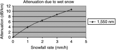
Figure 5.4. Dry snow: attenuation in function of snowfall
5.4.6. Scintillation
Randomly distributed cells of various sizes (10 cm to 1 km) and different temperature can be formed within the propagation medium under the influence of thermal turbulence. These different cells have different refractive indexes causing scattering, multiple paths, and variation in the angles of arrival: the received signal fluctuates rapidly at frequencies between 0.01 Hz and 200 Hz. The wave front varies similarly causing focusing and defocusing of the beam. Such fluctuations of the signal are called scintillation.
Figure 5.5. Influence of a large turbulent cell (deviation)
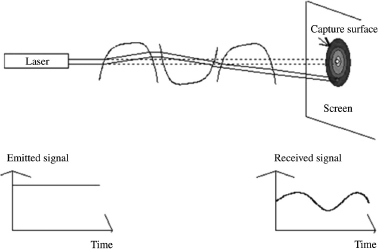
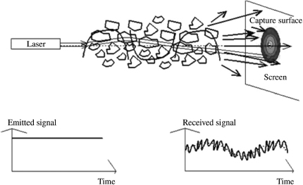
Figures 5.5–5.7 show schematically this effect as well as the variations (amplitude, frequency, etc.) of the received signal. The beam deviates when the heterogeneities are large compared to the beam cross section (Figure 5.5) and the beam is widened when heterogeneities are small (Figure 5.6). A mixture of heterogeneities results in scintillation (Figure 5.7) [WEI 08].
Figure 5.6. Influence of a small turbulent cell (widening of the beam)
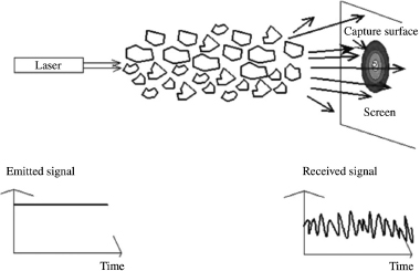
Figure 5.7. Heterogeneities (scintillations)
Tropospheric scintillation effects are usually studied from the logarithm of the amplitude ![]() [dB] of the observed signal (log-amplitude), defined as the ratio in decibels between the instantaneous amplitude and to its average value. The intensity and the fluctuations rate (scintillations frequency) increases with the frequency of the wave. For a plane wave, a weak turbulence, and a punctual receiver, the scintillation variance of “log-amplitude”
[dB] of the observed signal (log-amplitude), defined as the ratio in decibels between the instantaneous amplitude and to its average value. The intensity and the fluctuations rate (scintillations frequency) increases with the frequency of the wave. For a plane wave, a weak turbulence, and a punctual receiver, the scintillation variance of “log-amplitude” ![]() [dB2] can be expressed by the following relation:
[dB2] can be expressed by the following relation:
Equation 5.12. Scintillation variance
where
– k (2![]() /
/![]() ) is the wave number (m−1).
) is the wave number (m−1).
– L is the length of the link (m).
– ![]() is the refractive index structure parameter, the turbulence intensity (m−2/3).
is the refractive index structure parameter, the turbulence intensity (m−2/3).
The peak-to-peak amplitude scintillation is equal to ![]() and the attenuation due to the scintillation is equal to
and the attenuation due to the scintillation is equal to ![]() . For strong turbulence, there is a saturation of the variance given by the above relation [BAT 92]. Note that the parameter
. For strong turbulence, there is a saturation of the variance given by the above relation [BAT 92]. Note that the parameter ![]() has a different value at optical wave than at millimeter wave [VAS 97]. Millimeter waves are particularly sensitive to humidity fluctuation while at optical wavelength, the refractive index is essentially a function of temperature (the contribution of water vapor is negligible). At millimeter wavelength,
has a different value at optical wave than at millimeter wave [VAS 97]. Millimeter waves are particularly sensitive to humidity fluctuation while at optical wavelength, the refractive index is essentially a function of temperature (the contribution of water vapor is negligible). At millimeter wavelength, ![]() value is approximately equal to 10−13 m–2/3 which is a mean turbulent (usually in millimeter wavelength, we have
value is approximately equal to 10−13 m–2/3 which is a mean turbulent (usually in millimeter wavelength, we have ![]() ), and in optical wavelength,
), and in optical wavelength, ![]() value is approximately equal to 2 × 10⁻¹⁵ m−2/3 which is a weak turbulence (usually in optical wavelength, we have
value is approximately equal to 2 × 10⁻¹⁵ m−2/3 which is a weak turbulence (usually in optical wavelength, we have ![]() ) [BAT 92].
) [BAT 92].
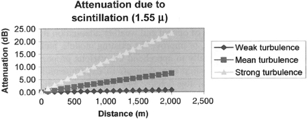
Figure 5.8 illustrates the variation of the attenuation of 1,550 nm wavelength optical beams for different types of turbulence over distances up to 2,000 m.
Figure 5.8. Variation of the attenuation due to scintillation
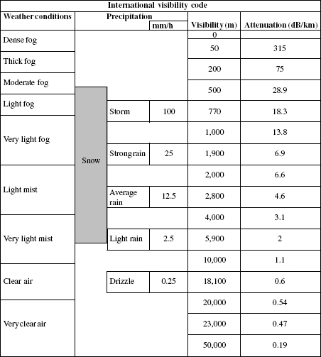
The international visibility code (Table 5.3) shows the attenuation (dB/km) for various climatic conditions [KIM 01]:
– weather conditions (from very clear periods to dense fog);
– precipitation (mm/h): drizzle, rain, storm;
– visibility from 50 km to 50 m.
Table 5.3. International visibility code
5.5. Experimental set-up
We describe below the experimental set-up carried out on the site of La Turbie (France) to characterize the optical propagation channel in the presence of different meteorological conditions (rain, hail, snow, fog, mist, etc.). The aim is multiple [NAB 04]:
– to study the influence of the atmosphere on the propagation of a laser beam (FSO);
– to compare atmospheric attenuation models against carried measurements;
– to determine the most reliable and most realistic attenuation model due to fog;
– to define the most robust wavelength.
It consists of:
– an FSO link operating at 650, 850, and 1,550 nm;
– a meteorological station;
– a transmissometer.
Figure 5.9 represents a synoptic view of the experimental set-up.
Figure 5.9. Synoptic view of the experimental set-up
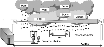
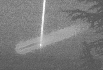
Figure 5.10 shows a picture of the transmissometer (narrow vertical beam) and of the 650 nm laser (divergent horizontal beam) light beam taken at night in the presence of dense fog.
Figure 5.10. Light beam of the transmissometer and laser
The implemented weather station is composed of the following sensors:
– a thermometer (outside temperature);
– a barometer (atmospheric pressure);
– a hygrometer (atmospheric humidity);
– an anemometer (instantaneous and average wind speed);
– a weather vane (wind direction);
– a rain gauge (rainfall);
– a pyranometer (solar radiation).
5.6. Experimental results
We present some experimental results (Figures 5.11 and 5.12) deduced from the measurements of attenuation in function of the visibility carried out under the project COST 270 in cooperation with the University of Graz (Austria) [GEB 04].
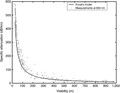
5.6.1. Comparaison with Kruse and Kim model (850 nm)
Figures 5.11 and 5.12 show the evolution of the measured attenuation at the site of La Turbie of the specific attenuation (dB/km) of the light beam at 850 nm in function of the visibility in the presence of fog.
The results are compared with Kruse and Kim models.
Figure 5.11. Measurements and comparison with Kruse’s model
5.6.2. Comparaison with Al Naboulsi’s model
Figures 5.13 and 5.14 show the evolution of the measured attenuation at the site of La Turbie of specific attenuation (dB/km) of the light beam at 850 nm in function of the visibility in the presence of fog.
The results are compared with Al Naboulsi’s models (advection and convection).
Figure 5.12. Measurements and comparison with Kim’s model
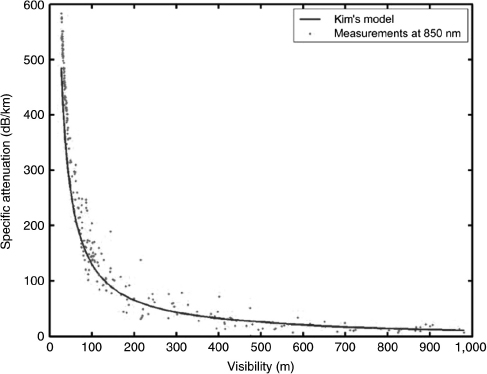
Figure 5.13. Measurements and comparison against Al Naboulsi’s model (advection)
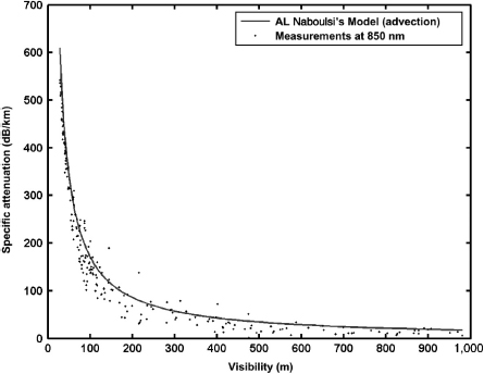
Figure 5.14. Measurements and comparison against Al Naboulsi’s model (convection)
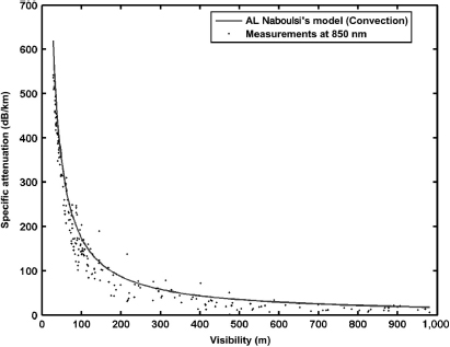
Measurement comparisons to existing models in the literature shows a good agreement between measurements and models available.
From analysis of the previous curves, it appears that the Al Naboulsi model, developed from FASCOD, is in excellent agreement with experimental measurements for low visibility while Kruse and Kim models deviate significantly from the measurements.
5.7. Fog, haze and mist
Fog, haze, and mist are composed of fine water droplets (<100 μm) suspended in the air. In some very cold countries, they can be particles of ice. It is formed by a process of condensation near the ground resulting from a radiative cooling of the earth (especially at night) or the passage of air on a cold ground (advection fog or advection mist).
To distinguish fog from haze or mist, it is generally agreed that the visibility is greater than 1,000 m in the presence of haze while it is less than 1,000 m in the presence of fog. Their compositions and their size distributions vary widely. In general, fogs have a water content lower than clouds (<0.1 gm−3) and a smaller concentration of droplets (<100 cm−3). It is characterized by visibility, determined by the maximum distance beyond which a prominent object cannot be seen by a human observer. The occurrence of fog is very variable depending on location, proximity to the sea or a large lake, mountainous zones, etc.
The liquid water concentration in the fog is typically equal to about 0.05 g/m3 for a moderate fog (visibility of about 300 m) and 0.5 g/m3 for dense fog (visibility of about 50 m) [ITU 05].
NOTE:— Meteorological measurements carried out in Belgium on 16 stations in 20 years provide information on its maximum (worst case) and median (not exceeded in 50% of cases) annual frequency. Table 5.4 gives the annual frequency of these fog events [BOD 77].
Table 5.4. Annual frequency of fog events in Belgium
| Median frequency (%) |
Maximal frequency (%) |
|
| Light, moderate, or thick fog (V < 1,000 m) | 0.055 | 0.14 |
| Moderate or thick fog (V < 500 m) | 0.035 | 0.11 |
| Thick fog (V < 200 m) | 0.020 | 0.08 |
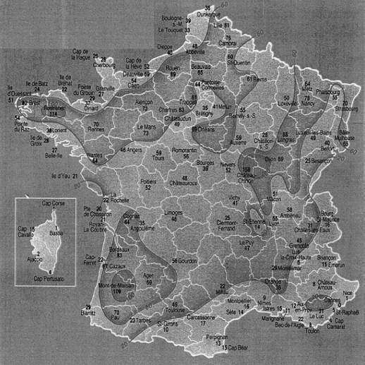
Figure 5.15 shows the distribution in France of the number of days per year with the presence of fog (days during which there is, even temporarily, a reduction in visibility to less than 1 km).
5.8. The runway visual range (RVR)
5.8.1. The visibility
Originally defined for the purposes of meteorology, the RVR (or visibility) is the distance for which a parallel luminous ray beam, generated by an incandescent lamp, at a color temperature of 2,700 K, must cover so that the luminous flux intensity is reduced to 0.05 of its initial value. It characterizes the transparency of the atmosphere.
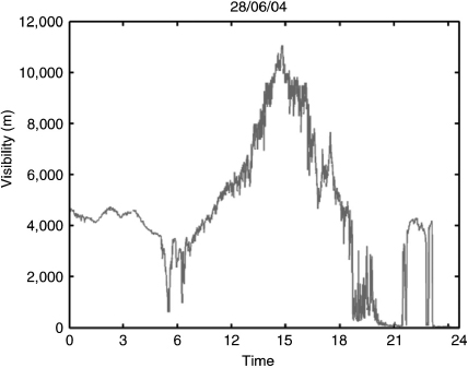
Figure 5.16 provides an example of changes in the RVR observed at the site of La Turbie (06) 28 June 2004 during a day of low visibility (<10,000 m) and in the presence of fog (<1,000 m).
Figure 5.15. Distribution in France of the number of days with fog per year
It is measured using a transmissometer or a scatterometer. The transmissometer is an instrument based on the loss of light intensity of a beam of light rays in the atmosphere, which depends on both absorption and diffusion.
The scatterometer gives an indication of the visibility in the atmosphere by measuring the diffusion of a beam light from a given volume.
Figure 5.16. RVR variations observed on the site of La Turbie
5.8.2. Measuring instruments
5.8.2.1. The transmissometer
The transmissometric method is the most commonly used to measure the average extinction coefficient in an horizontal air cylinder placed between a transmitter with a modulated light source and a receiver with a photodetector (usually a photodiode located at the parabolic mirror or a lens focal point).
The halogen lamp or the light discharge tube in the xenon is the most commonly used light source. The modulation of the light source avoids the influence of the solar flare.
The current from the photodetector determines the transmission factor which is used to calculate the extinction coefficient and the RVR.
There are two types of transmissometer [COJ 99]:
– Those where the transmitter and the receiver are placed in different cases and at a known distance from each other (Figure 5.17).
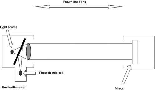
– Those where the transmitter and the receiver are placed in the same case, the emitted light is reflected by a remotely placed mirror or retro reflector (Figure 5.18).
Figure 5.17. Direct beam transmissometer
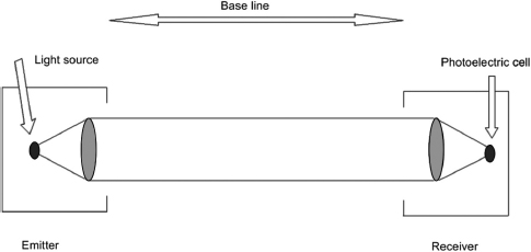
Figure 5.18. Reflected beam transmissometer
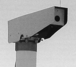
The distance covered by the light between the transmitter and the receiver is commonly called “the transmissometer base” and can vary from a few meters up to 300 m. Figure 5.19 shows the emission part of a transmissometer installed on the site of La Turbie during the experiment carried out to study the effects of fog on the visible and infrared propagation of FSO in the Earth’s atmosphere.
Figure 5.19. Emission part of a transmissometer installed on the site of La Turbie
5.8.2.2. The scatterometer
The most convenient method to perform this measurement is to focus a light beam on a small volume of air and determining, by photometric means, the proportion of light scattered in a large enough solid angle and in not preferred directions.
Two types of measurement are used in these instruments: backscatter and forward scatter [COJ 99].
Backscatter (Figure 5.20): The light beam is concentrated in a small volume of air; it is backscattered and collected by the photoelectric cell.
Figure 5.20. Schematic representation of the visibility measurement by backscatter
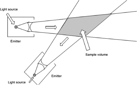
Forward scatter: The instruments consist of a transmitter and a receiver whose emission and reception beams form between them an angle between 20° and 50° (Figure 5.21). Other devices place a diaphragm halfway between the transmitter and the receiver, or two diaphragms placed close to the transmitter and the receiver.
Figure 5.21. Schematic representation of the measurement of forward scatter visibility
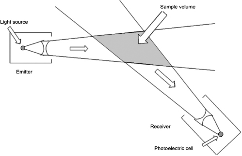
Figure 5.22. Example of a scatterometer implemented on a motorway area
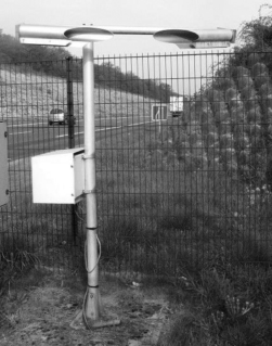
Figure 5.22 shows a photo of a scatterometer implemented on a motorway area to measure the fog intensity and announce to motorists the atmospheric visibility.
The knowledge of the visibility finds numerous applications in meteorology (identification of an air mass for synoptic meteorology and climatology), in aeronautics (determination of RVR), in telecommunications (evaluation of the effects of atmospheric particles (fog and aerosols) on optical, visible, and near-infrared transmission until 2.5 µm, determination of FSO links in presence of fog more particularly), and in terrestrial or maritime traffic security (measurement of the visibility in the fog) [DEF 07, DEF 10, HAU 05, HAU 06].
5.9. Calculating process of an FSO link availability
Software simulating FSO link in terms of probability of availability or interruption (QoS) has been developed at Orange Labs [ORA 11, CHA 05]. It is a decision support tool for the development of point-to-point high-rate FSO links over short distances. It includes data on the equipment (power, wavelength, sensitivity, etc.), the location of a site (coordinates, altitude, height/ground, etc.), and climatic and atmospheric parameters (relative humidity, soil roughness, albedo, solar radiation, etc.). It relies on the available technical knowledge relative to the effects of aerosols, scintillation, ambient light, rain, etc., the proprietary algorithms to model impairments due to snow or visibilities below 1 km, and the important phenomena such as advection and convection fog, weather statistics, and experiments analysis results. Applied to an experimental link, the results derived from the software showed excellent agreement between the predicted and the effective availability [NAB 05].
Three screens characterize the software: input data acquisition, results, and link profile presentation.
– The input data acquisition screen allows us to enter the following information (Figure 5.23):
– the data defining the link physical location (latitude, longitude, altitude, height above ground, orientation, etc.);
– the data characterizing the used equipment (number of transmitters, power, diameter, divergence, etc.);
– the data providing environmental information of the site (relative humidity, albedo (percentage of reflected solar energy), roughness, solar radiation, distance, etc.);
– the equipment data (wavelength, rate, system loss, etc.);
– the environment (urban, rural, marine).
Figure 5.23. Input data acquisition screen
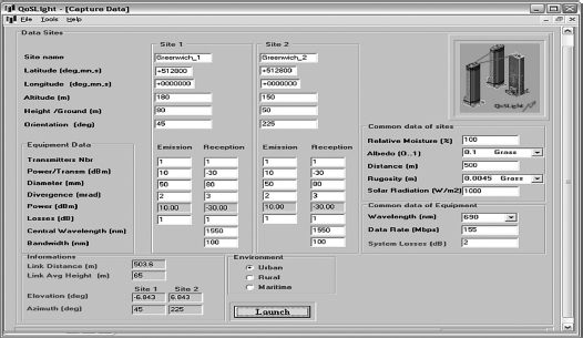
Figure 5.24. Results presentation screen
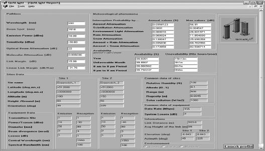
The results presentation screen displays the following results (Figure 5.24):
– the link information (length, medium height, elevation, azimuth, etc.);
– weather information;
– the data sites (equipment, environment, etc.);
– the link availability and the interruption probability.
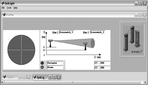
The profile screen shows the wave front propagation (Figure 5.25).
Figure 5.25. Screen showing the wave front propagation
5.10. Conclusion
The various aspects of the photon propagation in the atmosphere have been presented (molecular and aerosol absorption, molecular and aerosol diffusion (hail, smoke, haze, fog), rain and snow attenuation, and scintillation effects). They are the key to any good understanding of future communication systems using wireless optical links. Fog seems to be the most detrimental element to the operation of FSO links.
The comparison of experimental data allowed us to validate propagation models proposed in the literature. These are used to control transmission power levels of future FSO links by ensuring a sufficient momentum taking into account the variability of optical propagation conditions.
Experimental links showed that the FSO is a reliable broadband alternative to laying optic fiber and leads to greater acceptance of this technology in the industry of high-rate telecommunications networks.
To better understand the availability of an FSO link, the reader is referred to quality of service simulation tools. These tools allow us, for a given geographic site, to determine the availability and reliability of a link based on system parameters (power, wavelength, and equipment characteristics) and climatic and atmospheric parameters. They integrate the various physical phenomena responsible for the link blackout, such as attenuation due to ambient light, scintillation, rain, snow, and fog. Practical examples are provided in Chapter 11.
These various elements described in this chapter have contributed to the development of new recommendations at International Telecommunication Union (ITU), dedicated to propagation data and prediction methods required for the design of terrestrial FSO links [ITU 03, ITU 07a, ITU 07b].
The laser beam propagation in the atmosphere has been studied extensively in recent years. Many items are available in the literature. The reader can refer to them in [LEI 03, WAI 05, GRA 07, POP 09, WAL 09, STO 09, HEN 10].