Chapter 6

Indoor Optic Link Budget

6.1. Emission and reception parameters

For indoor (propagation limited to contours of a room) or outdoor communication, a detailed analysis of the assessment of connection (link budget) is a very significant step for any system. For example, for the systems with optical fibers, the engineer examines the power which is injected into fiber by the transmitter and then determines all the potential losses and gains until the signal arrives on the reception device. The receiver typically has a specific sensitivity (S_e) to a given throughput. This sensitivity represents the lower limit of the optical level of power rather than the reception for a quality of preset transmission. To guarantee the required quality of service (QoS), it is necessary to make sure that after having withdrawn all the losses, the received power remains above the sensitivity of the receiver. To make the connection more resistant, it is judicious to work on a level of power in reception slightly higher than the necessary minimum capacity: the variation is called margin and constitutes a reserve of power used in the event of degradation of the channel. This step represents the compromise between the distance from transmission and the reliability of the communication.

Like the devices in the field of radio or fiber optics, this process is similar for optical wireless systems.

In general, the principal parameters to be taken into account are:

– optical power transmitted by source (P_t), whose values range from 0 (1 mW) to 30 (1 W) dBm according to the wavelength and cost of the emission module;

– the divergence of the emission beam (DIV), whose total value should be of approximately 90° or ±45°;

– the sensitivity of the receiver (S_e), whose values range from –90 (1 nW) to –20 (10 μw) dBm according to the throughput and the detection surface;

– the effective surface of reception (A_eff), which generally includes the active surface of the receptor and an optical antenna of concentration;

– the aperture of receptor (field of view — FOV), whose total value should also be of approximately 90° or ±45°;

– the positions and the distance from the couple transmitter/receiver.

NOTE.— The reader will find further information relating to the elements of geometrical optics, photometry, and energy, and to the logarithmic notation, respectively, in Appendices 1 and 2.

Before reaching the receptor, the optical beam is attenuated. To understand how part of the transmitted power arrives at the receptor, it is necessary to examine the various losses in the wireless optical channel. The losses to be considered are:

The optical losses: This is mainly due to the imperfect lenses and the losses due to interfaces. This attenuation is generally integrated in the value of transmitted power (P_t) or the sensitivity (S_e).

The loss of pointing: For indoor environments, these effects are supposed to be negligible.

The atmospheric loss: In the event of significant atmospheric scintillation, it is possible to have a degradation of the signal. But the distance considered in an interior environment makes this attenuation negligible.

The molecular loss: This represents the attenuation by the molecules of the atmosphere. This attenuation is a function of the used wavelength. But their linear values are sufficiently low (maximum 0.41 dB/km at 850 nm) to be also regarded as negligible for indoor environment.

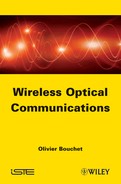
The geometrical loss: This attenuation is due mainly to the divergence of the optical beam, the distance, and the effective reception surface. The geometrical attenuation is the most significant loss. For example, with identical parameters of P_t, S_e, and A_eff, therefore the same value of geometrical attenuation, then three values of divergence (DIV equivalent to ±1⁰, ±15⁰, and ±80°); Figure 6.1 shows the various values of the maximum distance on the normal axis of connection.

The maximum distance varies very quickly with the value of the divergence. For a given value of the divergence, when the distance is doubled, the geometrical attenuation is quadrupled. A low divergence is generally used in the point-to-point outside communications (free-space optics — FSO) whereas a strong divergence is used for the remote controls.

6.1.1. Transmission device: parameters

One of the significant points relates to the calculation of the emitted optical power, and the way in which this power is connected to the light intensity, quantity varying according to the direction. The emitted optical power is the integral of the light intensity on all the directions of emission. The intensity of its radiation I(, ) is defined like the power per solid angle unit emitted by the source with the position (, ) compared to its normal.

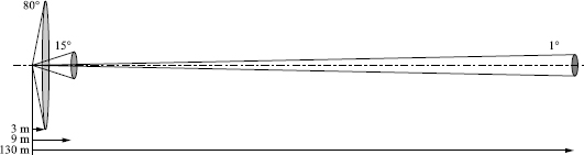
This is generally considered the case for a source, as shown in Figure 6.2, such as the power, which is radiated according to a circular symmetry around the vertical.

This figure represents the elements of the calculation of the optical power emitted on a solid angle equal to 2; the surface of the shaded zone is equal to dΩ).

Owing to this symmetry of revolution around its optical axis, the intensity of the source depends only on one Φ angle. We can then model it according to a generalized Lambert model [GFE 79, BAR 93].

Indeed, to calculate the optical power emitted on a solid angle equal to 2 using such a source having a symmetry of revolution around its optical axis, we cut out the solid angle Ω in a succession of annular angles elementary dΩ ranging between the angles Φ and Φ + dΦ:

If the radiated power follows the generalized Lambert model, we will have the following equation:

Therefore, radiated total power P_t will be:

And the normal intensity radiated in the normal direction with the source of light is given by:

The device of emission will thus be characterized by two significant elements:

– the transmitted average optical power P_t (in mW or dBm);

– the half-power (HP) angle (in degrees) (optical transmitted HP angle).

This angle HP, such as the light intensity, lowers half and it indicates that the source can light uniformly in all the directions (Figure 6.3):

From this angle HP, it is possible to determine the parameter m:

Table 6.1 presents some m values for various values of HP for a generalized Lambert model.

In the case of a device with several systems of emission coupled, the ones with the others, in order to increase the divergence, we can consider, initially, an average value of total power and an HP angle including all the systems of emission.

From equations [6.2] and [6.4], it becomes possible to calculate the power radiated per solid unit of angle ():

Figure 6.4 shows an example of emission diagram with HP equal to 30°, then a divergence (DIV) at ±30°.

With an aim of obtaining a significant HP angle, it is possible to use optical diffusers in front of the source of emission, but this increase also gives a significant geometrical attenuation. The use of several sources (multisector) in three dimensions makes it possible to improve the total HP angle and the emission coverage.

6.1.2. Reception device

An optical reception device is made up mainly of an optical system to collect and concentrate the incident radiation, an optical filter making it possible to reject the optical disturbers, and a photodiode that converts the light intensity into electrical current. After these optic and electro-optic elements, there are additional amplification modules and data recovery in the electric field.

In complement of the sensitivity of the reception device expressed in mW or dBm, the effectiveness of the receptor is determined by two other significant elements: the effective surface of collection A_eff (mm²) and the aperture or the FOV corresponding to the direction exposed to 50% of the maximum of received intensity.

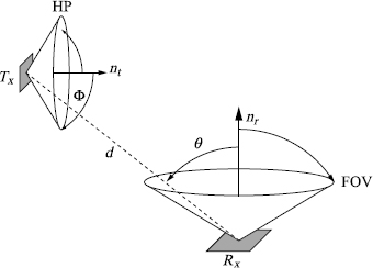
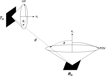
Figure 6.5 shows an example of a receptor (R_x) placed at a distance d of the emission source (T_x).

The optical device of reception (R_x) detects an optical power that is directly proportional to its effective light-collection area. Increasing the photodiode area is expensive, and tends to decrease receiver bandwidth and increase receiver noise. Hence, it is desirable to employ an optical concentrator to increase the effective area. Concentrators may be imaging or of the non-imaging variety. The imaging concentrator reproduces the image at the image focal point. The telescopes used in long-range, free-space optical links represent examples of imaging concentrators. The non-imaging concentrators are used for most short-range links. The majority of the indoor wireless optical systems are carried out with a non-imaging concentrator, such as a hemispherical or aspheric lens. The aspheric lens is a lens close to a portion of sphere but not strictly spherical.

For an incidence angle compared to the normal axis of receiver (R_x), an ideal non-imaging concentrator that has an index of refraction n has a gain of g() [BAR 94]:

In general, an optical filter is associated in order to reject the undesirable wavelengths and attenuate the ambient light as much as possible [KAH 97]. Their transfer functions T_f() depend on the angle of incidence. The value of the effective surface of collection of an optical receptor device (R_x), having a photodiode, an optical filter, and a concentrator, is given by the following equation:

The non-imaging concentrator represents the optimal solution between the effective surface and the aperture (FOV). By supposing an ideal optical filter with a transfer function corresponding to the unit, equation [6.9] can be rewritten as:

where

– A_eff is the maximum effective surface corresponding to a transmission with the normal (n_r) of the device of reception (R_x).

– rect (.) is a rectangular function defined by:

Beyond a certain angular value, the incident beam does not reach any more the active surface of the photodiode, as a result the communication is not carried out any more. This following relation is deduced from equation [6.10]:

This relation gives us the effective limit of collection surface available according to an FOV and a surface aperture of photodiode. An increase in the effective surface of collection induces an increase in the received power, but it reduces the FOV and thus the system coverage. A compromise is thus essential in the systems design.

The last significant parameter is the sensitivity of the optical receptor (S_e). It is the minimal value of received optical power allowing a correct detection of the transmitted signal. The sensitivity S_e corresponds to the detection threshold based on the dark current (I_d) of the photodiode. When the value of the optical power received on the active surface of the photodiode is lower than this sensitivity, the photodiode does not produce any answer. The sensitivity S_e is proportional to the responsivity (R), which is expressed in Ampere/Watt, and the dark current (I_d) in Ampere, and is given by the following expression:

The sensitivity S_e is expressed in dBm or mW. It depends mainly on the bandwidth (which is related to the active surface) and the photodiode type. For example, an APD photodiode with a spectral response (R) of 0.43 A/W at 830 nm and a dark current (I_d) of 0.5 nA has a theoretical sensitivity of −59 dBm.

Actually, the sensitivity of the receptor must take into account the losses of internal optics of the optical reception device, such as the concentrator or the filter. Moreover, the sensitivity of the reception device must also take into account the perturbation due to the ambient light, the thermal noise, the electric noises, and the losses in the electric circuits, such as the amplifiers. Thus, the value of sensitivity of an optical reception device including an APD, as mentioned above, becomes −36 dBm.

6.2. Link budget for line of sight communication

6.2.1. Geometrical attenuation

We describe a generic model of calculation for a line of sight (LOS) and wide line of sight (WLOS) link budget, allowing us to consider the devices as black boxes. This approach makes it possible to integrate the devices characteristics of filtering, concentration, optical divergence, and the losses of the emission and reception devices. We indicated that the most significant attenuation is the geometrical attenuation; therefore, this value is related to the transmitted average power (P_t) and the power received (P_r) by the following relation:

For the LOS and the WLOS having only one path, it is possible to calculate only H(0). Let us have a device of emission (Figure 6.5) whose emitted power is identical to generalized Lambert model. If we suppose that the value of the effective surface of the reception device (A_eff) is very low compared to the square of the distance from the couple transmitter/receptor (A_eff << d²), then it is possible to write the received average optical power as the following relation (the (Φ) angle is the angle between the normal axis of the source (n_t) and the direct path):

From relations [6.7] and [6.15], we obtain:

Consequently, for an LOS or a WLOS, the channel gain (direct current) or the linear geometrical loss is given by:

The corresponding impulse response can be comparable with a simple filter defined by [BAR 93]:

6.2.2. Optical margin

The optical margin of a connection M_l (dB) is the difference between the power available in reception and the receptor sensitivity:

It is pointed out that a relatively high margin implies a high reliability of a wireless optical communication system, but that is with the detriment of the connection distance. Indeed, to assign most of the power of the signal to the margin of the system induces a reduction in power available in LOS with the distance. In fact, it is advisable to have a compromise between the distance and the reliability.

6.2.3. Coverage

Within the framework of a connection in LOS or WLOS, the coverage surface (A_c) can be defined for an angular value corresponding to HP (at −3dB or 50%). It can be expressed in the following way (in m²):

For example, the coverage surface of an emission device, with an HP angle of 30° and a distance d of 2 m, will be 4.2 m².

6.2.4. Reciprocity and not reciprocity of the channel

An indoor wireless optical communication is symmetrical when the emission and reception apparatuses are identical and have the same optical characteristics, and the characteristics of the uplink and the downlink are similar. However, unlike the radio, it is generally supposed that a base station, in a part, communicating with one or more modules will not have the same parameters with respect to the modules. The parameters of the uplinks and downlinks are not equal any more. To illustrate this, we suppose a base station (BS) and a module (Mo) in a topology in LOS or WLOS.

The emission–reception devices of the base station (BS) are characterized by:

– an emission power for the downlink;

– its radiant intensity I^BS (Φ^BS), where Φ^BS is the angle of emission compared to the axis normal of the BS;

– the effective surface of collection , where ^BS is the angle of reception compared to the axis normal of the BS and has the maximum value when the angle ^BS is null;

– the FOV FOV ^BS of the uplink.

The module (Mo) is also characterized by:

– an emission power for the downlink;

– its radiant intensity I^Mo (Φ^Mo) , where Φ^Mo is the angle of emission compared to the axis normal of the module;

– the effective surface of collection , where ^Mo is the angle of reception compared to the axis normal of the module and has the maximum value when the angle ^Mo is null;

– the FOV FOV ^Mo of the downlink.

When dimensions of the base station and the module are supposed as small as possible, the distance d is relatively identical for the downlink and the uplink in a given configuration. We obtain:

– for the downlink:

– for the uplink:

Based on equation [6.18], the gain will be thus (equivalent to the loss of propagation between transmitter and receiver):

in which m^BS and m^Mo are, respectively, the numbers of mode from the base station and the module determined by their HP angle.

In diffusion mode (DIF) propagation, it is advisable to take into account the gains for each path. For indoor wireless optical communication, the channel gains of the downlink and of the uplink are generally different because of this asymmetry. The link budget evaluation must be calculated in two directions.

In the radio field, one antenna can be used for transmission and reception. In this configuration, the two responses are identical and the channel is reciprocal. In this case, the calculation of the channel gain in the downlink is the same calculation as the uplink. A similar configuration for optical wireless devices would facilitate the calculation process.

6.3. Link budget for communication with retroreflectors

6.3.1. Principle of operation

A retroreflector is a passive optic component that reflects the incidental light in the exactly opposite direction of this incident beam. The retroreflector generally has a large angle of vision (FOV). It is, for example, about ±12° for glass retroreflectors. The association of several retroreflectors makes it possible to increase the value of the field of vision.

The retroreflectors can also act as optical communication systems. If a retroreflector is associated with an electro-optical obturator on the cubic corner, it is possible to obtain a wireless optical communication. Indeed, the considered retrobeam can be activated or deactivated or at least modulated. By the assembly of a modulating retroreflector (MRR), we can allow the data transmission without the use of a light source such as laser or LED. For example, the basic station lights a module with a continuous or modulated optical beam. This beam arrives on the reflecting module and is passively considered toward the base station. The obturator, activated or deactivated by an electric signal, allows the transmission of the data coming from the module. This reflected signal containing the data from the module enters the receiver part of the base station to be treated. Figure 6.6 shows the diagram of an MRR.

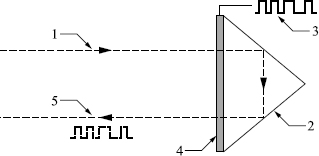
The principle of retroreflexion is defined by an incidental beam (1) which is reflected on the cubic corner (2). A numerical signal (3) is treated by an electro-optical obturator (4) in order to transmit a modulated signal (5). The reflected beam is in the same direction as the incidental beam. The advantages of this system are that it is light, compact, and energy saving. Moreover, the retroreflexion is insensitive with possible micromovements to the base station and to its orientation.

6.3.2. Optical budget

The calculation of the optical budget described below is defined for a retroreflector of cubic corner type with an optical device called “cats eye” with which the reflectivity of the beam is most effective. Indeed, precise alignment is not necessary and such systems reflect the incidental beam independently of the exact orientation of the reflectors.

In such a wireless optical system, the optical beam is initially emitted from a base station A with a definite divergence in order to cover the zone in which is located the retroreflector B. This module receives part of the emitted beam, then reflects it under another observation angle. This reflected beam arrives then on the device of reception of the base station A.

In the literature, several authors examined the geometrical factors which affect the relation between the transmitted power and the received power [LEO 91, LAS 01, ACH 04].

The starting assumption is a complete coverage of the incident beam coming from the base station A on the module B.

An optical beam is emitted from an emission device A with a diameter of transmission d_t and a divergence angle Φ_t (radians). It illuminates completely a module B at a distance D (Figure 6.7).

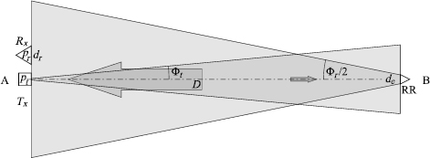
The reflected beam coming from the reflectors will have an effective diameter d_re and a divergence Φ_r (in radians) equivalent to the divergence of the transmitted beam and effects of diffraction due to the limited size of the reflectors. By supposing 100% of reflectivity of the reflectors and taking into account of a factor T corresponding to the atmospheric attenuation, the general formula of the received power P_r by device A on the effective surface of detection having a diameter d_r is given by:

It is obvious that distance D is a significant parameter for the value of the received power. For systems of short distance, the atmospheric or molecular attenuation T is negligible and that:

Then by preserving the Φ_r term, equation [6.22] can be reduced to [ALH 06]:

As an example and with the values indicated in Table 6.2, we note that at a distance of 1 m, the received power is 0.01% compared to the emitted power. In the same way, when an optical source in A (Figure 6.7) emits 100 mW (20 dBm) with a divergence of ±3 mrad, the detection device in A will receive 0.01 mW (−20 dBm).

Table 6.2. Optical budget, typical values

Parameters	Values
Distance — D (m)	3
Diameter of the receiver effective surfaces — dr (mm)	2
Diameter of the retroreflector — dre (mm)	8
Divergence of the reflected beam — Φr (mrad)	24
Divergence of the transmitted beam — Φt (mrad)	6
Diameter of the transmitted beam — dt (mm)	2

In this example, the losses due to the surface reflexions, glass absorptions, and interface losses are not taken into account. It indicates the best performance of the device.

6.4. Examples of optical budget and signal-to-noise ratio (SNR)

In the following examples, we propose to calculate the optical margin for several systems in various configurations. These simulations are carried out using the software QOFI, adapted for wireless optical communications. It is a tool for simulation in three dimensions [TEC 11]. It makes it possible to simulate optical devices for wireless communications in confined space with calculation of the geometrical attenuation, the impulse response of the channel, and the coverage zone in a furnished room. This application makes it possible for the user to create an interior and a 3D model by dimensioning a room with the insertion of furniture, the base stations, and the modules. It proposes calculations in LOS, WLOS, and DIF while integrating:

– the room dimensions, reflexion of the room, the floor, and the ceiling;

– the object dimensions, their position and orientation with their reflexion properties.

This software is based on the Nettle’s model, the technical details can be found in [BOU 08], and it is free downloadable via Internet sites [BER 08] or [QOF 11]. Table 6.3 presents several examples of wireless optical systems as shown in Figure 6.8. It supposes a power of emission of class 1, an ideal filter of transmission with a transfer function equal to 1, an ideal concentrator with a refraction index n of 1.52, and one OOK-NRZ modulation.

6.4.1. Examples of optical budget

Case 1 (WLOS): the bandwidth is 10 MHz, an OOK-NRZ modulation, a throughput of 10 Mbps, and the transmitter and the receiver are located on their respective normals (Φ and are null);

Case 2 (diffusion): the bandwidth is 10 MHz, an OOK-NRZ modulation, a throughput of 10 Mbps, and with retroreflectors (d_re = 10 mm, Φ_r = 30 mrad, and d_t = 4 mm);

Case 3 (WLOS): the bandwidth is 100 MHz, an OOK-NRZ modulation, a throughput of 100 Mbps, and the transmitter and the receiver are located on their respective normals;

Case 4 (WLOS with a part of diffusion): the bandwidth is 100 MHz, an OOK-NRZ modulation, a throughput of 100 Mbps in LOS, and a diffusion (wall and ceiling: painting, ground: parquet floor, T_x and R_x to 1 m of the wall and the ground), the transmitter and the receiver are located at angles different from their respective normals;

Case 5 (LOS): the bandwidth is 1,000 MHz, an OOK-NRZ modulation, a throughput of 1 Gbps, and the transmitter and the receiver are located on their respective normals.

Figure 6.9 shows the characteristics of the impulse response in case 4.

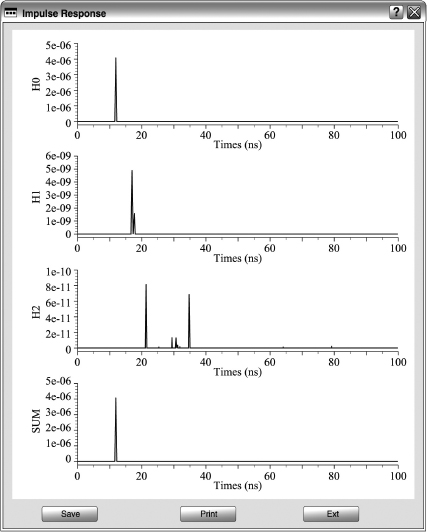
The contribution of the diffusion is the sum of the H1 (sum of the signals received with one reflexion) and H2 (sum of the signals received with two reflexions) curves. It accounts for only 0.01 dB in the margin link and created no intersymbol interference (ISI).

6.4.2. Examples of SNR and BER

From the expression of the SNR (signal-to-noise ratio, equation [4.12]), it is possible to present typical values of a wireless optical system in the case of an OOK-NRZ modulation:

where

– R represents the proportionality factor of optic/electric conversion (or spectral sensitivity), for example R = 0.6 (A/W).

– H(0) is the channel gain at the null frequency or the attenuation of the average optical power, for example H(0) = 3.03.10⁻⁶.

– P_t is the transmitted average optical power, for example P_t = 10 mW (10 dBm).

– P_b is the noise power.

– q = 1.6 x 10⁻¹⁹ C_b, is the electron charge.

– B is the binary rate, for example B = 150 Mbps.

The binary error rate (BER) is a value relating to the error rate measured with the reception of a digital transmission. It is in correspondence with the attenuations or the level of disturbance of a signal transmitted in the channel. It is given by the following formula:

We search the values of SNR and BER for various values of the power of the ambient light. Table 6.4 presents these values with a QoS indication.

A significant value of the ambient optical noise can induce a degradation of the system. An increase in the optical assessment makes it possible to correct it. That is, translated, for example, with an increase in the sensitivity in reception, a reduction in divergence (DIV) in emission, or an increase in the emitted power.

Concerning the two parameters in emission, there is nevertheless a limitation of these values because of the regulation on safety with respect to the people. This element is in particular developed in Chapter 7.