
Chapter 4
Assessment of Quality of 3D Displays
Quality is assessed by objective and by subjective criteria. Objective criteria are centered around disparity, depth, luminance, contrast, gray shades, and values of the color components such as location in the chromaticity diagram or the noise level in an image. Subjective criteria are harder to define but are subsumed under the perception of structural similarities or the reality of a depth perception.
Objective measures such as the peak signal to noise ratio (PSNR) [1, 2] are virtually not correlated to the quality perceived by the human visual system (HVS), while subjective measures are. The investigation of structural similarities is motivated by the observation that the HVS is highly adapted to detect structural differences, especially in structures that are spatially proximate [3, 4].
Algorithms providing quality information are as a rule based on area-wise or even pixel-wise comparisons between a reference image and the image to be characterized, or between the right eye image and the left eye image, or between two neighboring areas in an image. In this context also comparisons between different properties arise such as contrast or luminance in neighboring pixels or the luminance of an object compared to the luminance in the background.
In 2D and 3D displays the investigation of disparity or depth associated with the pixels or the areas in an image plays a dominant role. It provides depth maps and disparity space images (DSI) [5].
Extraction of the depth from a 2D image allows for the construction of a 3D image pertaining to the given 2D image. The determination of depth or disparity in a 3D image is based on differences between the right and left eye images. The ensuing depth or disparity maps are coded in gray shades: as a rule the brighter the shade, the smaller the depth or the larger the disparity. For a 3D image this disparity map and the 2D image pertaining to it can be transmitted in TV broadcasting requiring less bandwidth than the original 3D image. The reason is that the broadcast of the 3D image involves the transmission of two color images, one for each eye, each with a wealth of contrast, gray shade, and chrominance information, while on the other hand this wealth of information would only be contained in the transmission of one single 3D image, and the depth map required consists of color-free gray shades. At the receiving end the original 3D image has to be reconstructed. The pertinent technique described later in this section is called depth image-based rendering (DIBR).
Work on image quality was started by computer scientists who needed to enhance images on computer screens. The availability of 3D images for TV, medical imaging, and mobile (cell) phones has also prompted interest in the enhancement of quality in the display development and manufacturing area. The main interests in quality issues are acquisition, image display for mobile phones and TV, image compression, restoration and enhancement, as well as in printing.
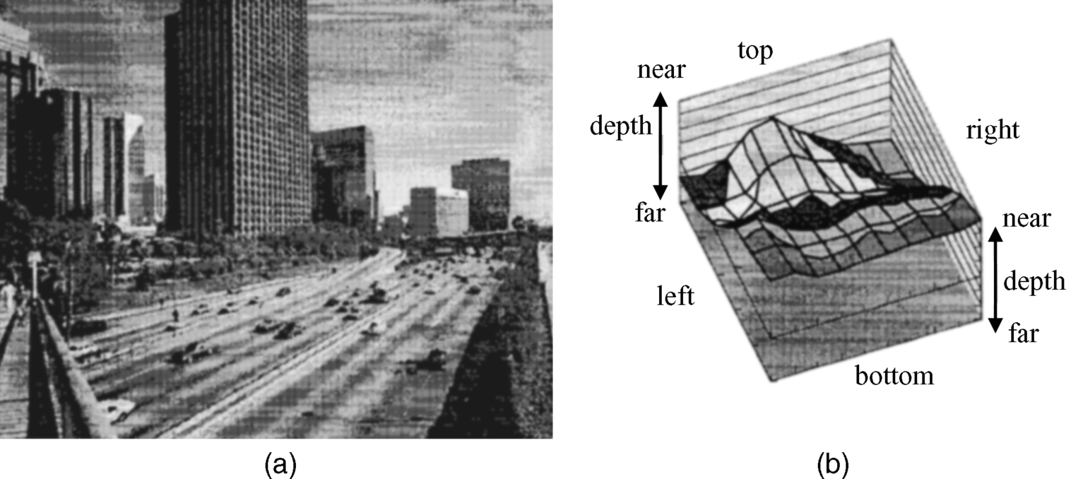
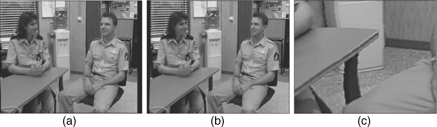
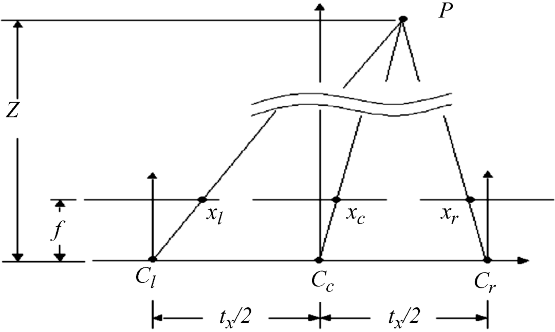
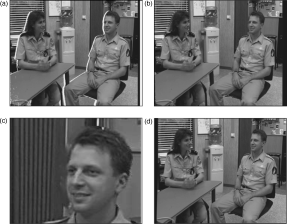
As we have to deal mainly with the disparity d and the depth z as a measure for the distance of an object, we now establish a relationship between the two derived from the data in Figure 4.1. This figure is similar to the arrangement of lenticular lenses with a pitch b in Figure 3.4 in front of an image on an LCD screen or on a CCD. When the eyes with interocular distance b in Figure 4.1 focus on point Q in the depth z, the axis of the right eye is rotated by an angle γ2 in Figure 1.1 out of the fovea corresponding to the length of the stretch xr on the LCD in Figure 4.1, while the left eye is rotated by γ1 in Figure 1.1 in the opposite direction of γ2 and hence corresponding to a negative length of the stretch −xl on the LCD in Figure 4.1. There, tan α and tan β provide the focal length f of the lenses
(4.1a)![]()
where k is the distance between the focus point and the axis of the left lens. Further, we obtain
(4.1b)![]()
yielding as the disparity
Figure 4.1 The relationship between the disparity d and the depth z of a point Q.
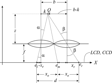
The disparity as the difference γ2 − γ1 in Figure 1.1 is not identical to Equation 4.1c but corresponds to the difference of the lengths xr − xl and finally also to the distance between el and er in Figure 4.1. So determining d also yields the depth z.
In the case of two cameras for the capture of images, the distance between the two cameras, also called the base length, plays the role of the interocular distance b of the eyes. This will be used in Figure 4.27.
In Figure 4.1 the points er and el on the x-axis indicate the placement of the pixels on the LCD screen belonging to the two images needed for 3D. At x = er the center pixels for the right eye image are located, while at x = el the center pixels for the left eye image are placed. For the LCD or CCD the distance em in the middle between er and el is important: em is exactly in the middle as it lies on the straight line from Q to the middle between the lenses with b/2 at each side. The distance from em to er and el is denoted by x0. Then we get the following equations:
![]()
from which the following is obtained also with Figure 4.1
![]()
which with Equation 4.1c provides
(4.1d)![]()
resulting with the first two unnumbered equations above in
and
We shall need Equations 4.1e, f later for the reconstruction of a 3D image.
The next sections are devoted to retrieving quality data, mainly disparity and depth, from given images; to similarities as subjective quality measures; to algorithms for establishing depth maps for 2D and 3D images based on objective and subjective quality measures; and to the reconstruction of 3D images from depth maps and 2D images.
4.2 Retrieving Quality Data from Given Images
This section is meant as a brief introduction to the considerations, process steps, and terminology of the methods used for extracting measured data from a given image. As it is also geared to providing data as perceived by the HVS, it is also interesting for algorithms designed for subjective criteria.
The process steps are listed in Figure 4.2[3]. The two input signals ej and ek, where j and k may be numbers of pixels, or the reference signal and the distorted signal of an image or a pixel, as well as any two signals for which a comparison is needed. In any case the difference
(4.2)![]()
is of interest. The processing performs a proper scaling which might, in the case of color, be transformed into a color space. A lowpass filter simulating the point spread function (PSF) of the HVS tailors the image to the form perceived by the eye. The PSF is the impulse response of the human eye with the Fourier transform being the optical transfer function (OTF) of the eye, which is lowpass. The block in Figure 4.2 of the contrast sensitivity function (CSF) describes the sensitivity of the HVS to different spatiotemporal frequencies which are present in the visual stimulus. The CSF is used to weigh the signal according to the different sensitivities for contrast. The channel decomposition separates the images into subbands, also called channels in the psychophysics literature, that are sensitive to special spatial and temporal frequencies. They are assumed to be related to the neural responses in the primary visual cortex [6, 7].
Figure 4.2 Signal processing for quality assessment of an image.
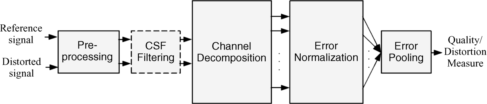
A normalization of ejk takes into account that the presence of an image component will decrease the visibility of another image component that is proximate in spatial and temporal location. The normalization weighs the signals by a space-varying visibility threshold [8]. This normalization is intended to convert the difference ejk into units of a just noticeable difference (JND). The final stage of error or difference pooling in Figure 4.2 adds the normalized signals from the space of the total image into a single value
(4.3)![]()
which is the Minkowski norm. For β = 2 we obtain the L2-norm, which is the mean square difference (MSD). The spatially variant weighing of ejk may be provided in a spatial map [9]. The exponent β may assume values from 1 to 4.
Some limitations on the characterization of an image by MSDs are now briefly itemized.
The MSD is a questionable measure for quality, because some differences may be clearly visible but are not considered to be objectionable on a subjective basis. The threshold of visibility of a difference may not be a psychologically correct value for the importance of perceptual distortions at larger difference levels. Most psychological experiments use simple patterns such as spots and bars. In images of greater complexity the masking phenomena, by which the visibility of some differences may be diminished or masked by other distortions, result in an imperfect judgment of differences. The Minkowski metric assumes that differences at different locations are statistically independent. However, it has been shown that a strong correlation exists between intra- and inter-channel wavelet coefficients of natural images [10]. Cognitive interaction problems such as eye movements or different instructions given by observers lead to different quality scores.
4.3 Algorithms Based on Objective Measures Providing Disparity or Depth Maps
4.3.1 The Algorithm Based on the Sum of Absolute Differences
In the left (L) eye and the right (R) eye image, the disparity in matching pixels will now be investigated. The difference in the disparities indicates, as described in Chapter 1 and in Equation 4.1c, the inverse of the depth of a point that the eyes have focused on. The larger the difference in the disparities, the closer the point. The differences are expressed as the sum related to the same pixels in the two images in a window around a center point. This renders the sum independent of random insignificant values. The sums were first formulated as the sum of squared intensity differences (SSD) [11], but experiments revealed that the sum of absolute intensity differences (SAD) [12] yielded better results.
We know from Section 2.5 that perceived contrasts, or from Section 3.5 that perceived intensities, are related by the HVS to perceived disparities or depths; larger intensities or contrasts indicate a smaller depth. However, further experiments demonstrated that the value of color components, such as the location in the chromaticity diagram, provided the best result so far for depth perception. Therefore the cost function of the SAD approach in Equation 4.4 was based on color parameters providing the following set of equations [12]:
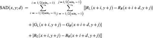
where x and y are the spatial coordinates of the images, d stands for disparity, also used as a search parameter in the right eye image, and winx and winy are the extensions of the search windows in the x- and y-directions.
We have to look at the meaning of d more closely. In Figure 1.1 the disparity has been introduced by the angles that the eyes are rotated from the fovea when they focus on a point at a given depth from the viewer. For points M and P on the horopter these angles γ are the same for both eyes, so the difference is zero. For points like Q closer to the viewer, the disparities γ1 and γ2 for the left and the right eye respectively are no longer the same, leading to a non-zero difference. This difference increases the closer Q is to the viewer. This difference in disparities is related to the parameter d in Equation 4.4 because the difference in the angles on the retina, measured in arcmin, is reproduced in the location of the pixels in the left and right eye images. The value of d is, of course, not identical to the difference of the disparities due to the mapping from the retina into the pixel domain, but is a good measure of the depth, being smaller for larger d. The interval for d is [dmin, dmax], where dmin = 0 is possible.
The search procedure starts with a given search window and a given estimated d for which the locations x, y in the image have to be found which minimize the SAD value. To achieve this, for each selected pair x, y its neighborhood has to be investigated by adding up the terms in Equation 4.4 for all i and j around the x, y pair in the search window. This has to be repeated for a dense enough grid of x, y pairs in the window. This defines the high computational load of the process. The solution is the minimum SAD value, because it provides the best match between the two images for a given d. This is also optically understandable as all other matches would entail a larger rotation of the axes of the eyes which is energetically unreasonable and also would not guarantee the quickest reaction.
The minimization of a cost function like SAD will be a characteristic of all other algorithms.
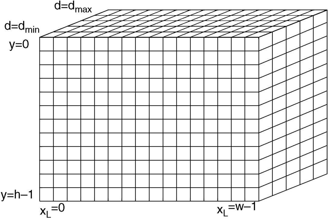
The match of the location x, y with the pertinent d is stored in the volume of a memory as shown in Figure 4.3.
Figure 4.3 Volume of a memory cube to store x, y, and the disparity d.
The search involves a wealth of computations which require efficient organization. An obvious feature is that the calculation for the next x-value deletes the previous x and adds one more x-value at the end, while the results for the x-values in between can be taken from the previous calculations. More helpful hints for efficiency are given in [12].
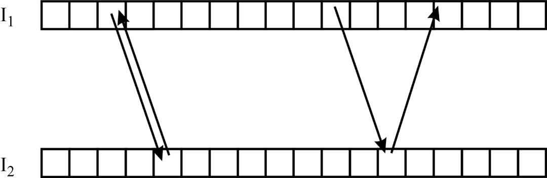
In order to avoid mismatches, validity tests for the matches have been introduced. One of the tests is the check on consistency at occlusions [13]. If a portion of a scene is visible in an image I1 in Figure 4.4 but not in image I2, the pixels in I1 corresponding to the occluded area in I2 will more or less randomly be matched to points in I2 which, on the other hand, correspond to different points in I1 and are matched with them. These matches are drawn on the right in Figure 4.4 as matches from I1 to I2 and from the same point in I2 to I1, but to a different point in I1. This is an inconsistency caused by the occlusion and the matches are therefore declared invalid. The consistency test on the left side in Figure 4.4 yields that the match from I2 leads to the same point in I1 as the original match from I1 to I2. These points meet the consistency tests and are declared valid.
Figure 4.4 Consistency check between two images I1 and I2.
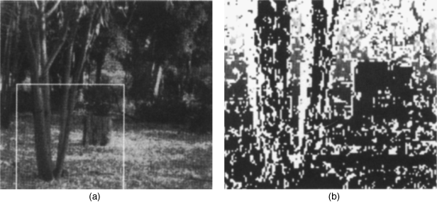
As an example Figure 4.5a shows in the section framed by the white lines a scene with trees, where the first tree occludes the area at the back. The disparity map in Figure 4.5b shows the occluded areas in white, while the deep-black areas are the farthest away.
Figure 4.5 A scene with trees framed by white lines in (a) and the disparity map in (b) with occlusions shown in white.
The consistency test for Equation 4.4 can be derived from the difference of the disparities in the two eyes, which are seen from the right eye in Figure 1.1 as ![]() and from the left eye as
and from the left eye as ![]() , so
, so ![]() holds. Translating the angles in corresponding distances dRL(x, y) and dLR(x, y) in the xy-plane in Equation 4.4 yields [12]
holds. Translating the angles in corresponding distances dRL(x, y) and dLR(x, y) in the xy-plane in Equation 4.4 yields [12]
(4.5)![]()
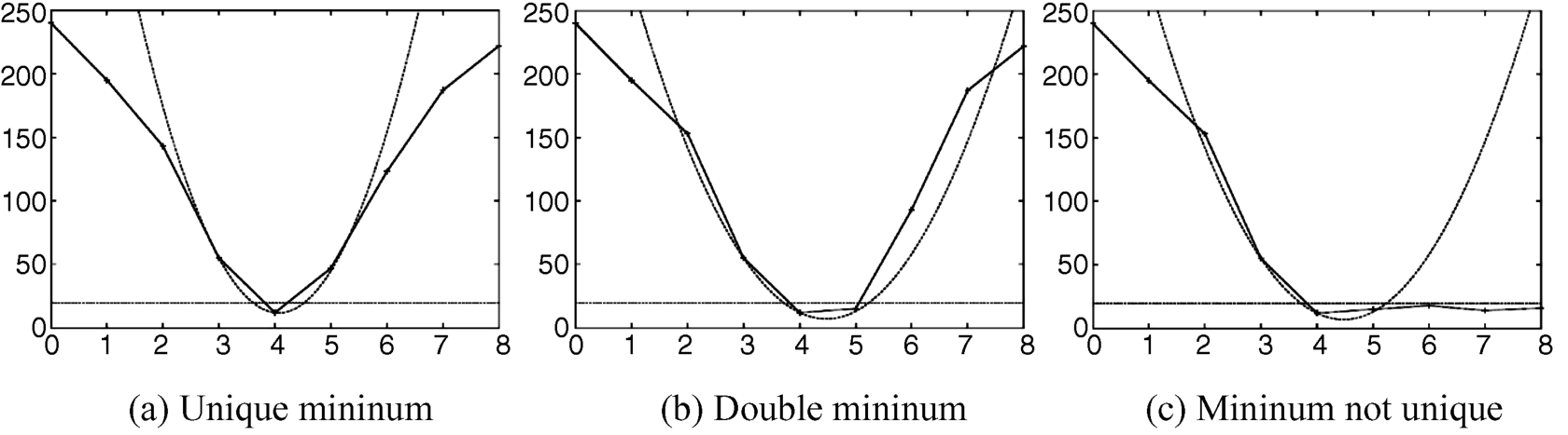
Due to the complexity of the information in an image with repetitive textures or without texture and with edges, a reliable matching is not always possible. So the uniqueness of a minimum of SAD is not guaranteed. The neighborhood around a minimum for x is investigated in Figure 4.6a–c by placing a parabola through the minimum and two more adjoining points [12]. The unique and the double minima are accepted, but the non-unique minimum is rejected.
Figure 4.6 Properties of a minimum of SAD, accepted for unique or double zeros, but rejected in (c).
A disparity map reached by SAD and also by other algorithms may exhibit salt and pepper noise which can be removed by a median filter. This noise is of course especially noticeable in weakly textured or untextured regions. A Gaussian filter with the transfer function
(4.6)![]()
where σ is the standard deviation, works in the domain of spatial frequencies fx and fy in the x- and y-directions and suppresses larger frequencies as a rule associated with noise, while the lower image frequencies are mainly preserved. Further, it cuts off the larger frequencies in sharp edges, abrupt steps, and in discontinuities, which results in a smoothing of the texture. The smoothing effect also tends to suppress isolated disparity points, so called outliers, which are found to be, as a rule, false matches. The Gaussian filter can also improve the results of SAD. In weakly textured or untextured regions, where the signal level and hence also the signal to noise ratio is low, the filter enhances the signal to noise level resulting in an improved SAD result.
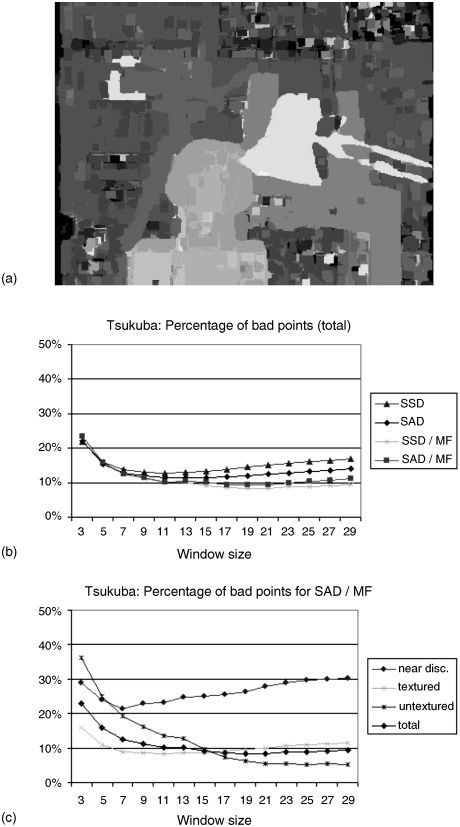
Figure 4.7a shows the widely used “Tsukuba” test image. The pertinent disparity map obtained by the SAD algorithm [12] is depicted in Figure 4.7b,c – the brighter the region, the closer the objects. The image in Figure 4.7b,c was median filtered [14]. It is noticeable that Figure 4.7b,c exhibits fewer background spots of noise.
Figure 4.7 (a) “Tsukuba” University test image. (b,c) Disparity maps of the Tsukuba test image in (a) without (b) and with (c) median filtering.
4.3.2 Smoothness and Edge Detection in Images
The necessity has arisen to find a cost function which improves the detection of edges and even of discontinuities in images. That would also support the investigation of weakly textured or even untextured regions by finding the borders of these regions which are edges. To this end an expanded cost function, also called an energy function, to be minimized, was introduced in [15] and enhanced in [16].
Before we proceed to the expanded cost function we have to clarify some terminology. The space with coordinates x, y, and d is called the disparity space, while an image or a function defined over a continuous or discretized disparity space x, y, d is a disparity space image (DSI). As an example SAD(x, y, d) is a DSI. If an algorithm works within a window, we have a local algorithm, such as SSD or SAD. If it works on the total image, we are faced with a global algorithm.
The enhanced cost function or energy function is [15, 16]
Edata measures the matching of data in two images as we know already from the DSI SAD(x, y, d) in Equation 4.4. So Edata is the initial matching cost function. The smoothness term is geared to enhance changes at the edges in an image. Edges are defined as points or regions exhibiting a large change in the properties of an image, such as intensities, gray shades, color components, or the depth, which the eye interprets as changes in disparities. In order to catch these changes the smoothness function is defined in its simplest form as
where ρ is a monotonic function with increasing d, such as a positive linear or a quadratic function of d. Equation 4.8 shows that the change of d is calculated for an increase of x and y by one unit, which could be an increase in a neighboring pixel.
These terms also indicate the smoothness of a disparity function, from where its name is derived. The parameter λ is a weighting factor.
If Esmooth is related to differences in intensities I(x, y) the function ρ is
(4.9)![]()
where the term with the double bars is the Minkowski norm. PI is a constant or spatially varying weight factor. At discontinuities PI < 1 can serve as a limiting factor curtailing values that are too large at the discontinuity. The difference in the disparities can work in the same way as well. The main purpose of ρ is the enhancement of the contribution to E(d) stemming from edges and discontinuities. A further means to deal with discontinuities is the selection of PI as
(4.10)![]()
where ΔI is the gradient of the intensity at the x, y location, while γ controls the dependency on this gradient. The minimization of the energy function ensuˇes a heavy load of calculations. Minimization methods include simulated annealing, max-flow/graph cut, winner-takes-all, and dynamic programming.
An application of Esmooth lies in the weakly textured or untextured regions of an image. In such a region an algorithm such as SAD without the term Esmooth fails, because the properties used in these algorithms, such as the color components or the intensity, are everywhere virtually the same. In this case SAD tends towards zero everywhere because the values in the differences used for matching are the same independent of the value of d.
After having established a disparity map d(x, y), a validity check is required. It can consist of a pixel-wise comparison to a known correct depth map dT(x, y) of the same image, the so-called truth data. The error in the truth data is expressed by the following equations. The RMS error is
(4.11a)![]()
where N is the total number of pixels x, y. The percentage of error is based on
(4.11b)![]()
with δ being the error limit, above which a bad match occurs; so P indicates the number of rejected matches.
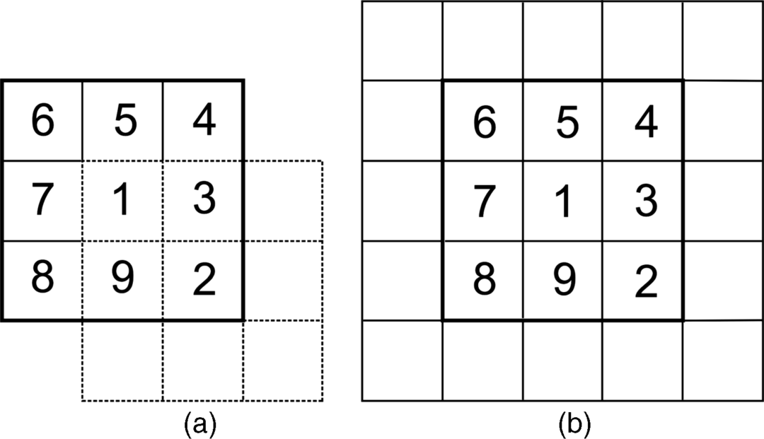
For the minimization of the number of rejected matches a min-filter (MF) is applied [16]. Its function is explained by the 3 × 3 windows in Figure 4.8a and 4.8b with the center being pixel 1. In order to find the pixel in the 3 × 3 window with the minimum contribution to the cost function, one has to evaluate all 3 × 3 windows which have one of the pixels in the original 3 × 3 window as its center pixel. Such a window is shown in Figure 4.8a with pixel 2 as its center pixel. All the pixels covered by these windows are shown in Figure 4.8b. The same area can be covered by shifting a 3 × 3 window into all positions around the center pixel 1. In this way, the pixel in the original window with the minimum contribution to the cost function is found.
Figure 4.8 (a) A 3 × 3 window of a min-filter with a search filter in dashed lines. (b) Area covered by all search filters containing the center pixel 1 of the min-filter.
Results provided by the minimizations of the cost function are presented in the disparity space image in Figure 4.9a and in the diagrams in Figure 4.9b and 4.9c. Figure 4.9a shows the disparity map of the Tsukuba test image in Figure 4.7a obtained by the SAD with the MF. The brighter the region, the closer the object. The diagrams in Figure 4.9b and 4.9c depict the percentage of rejected points versus the size of the search window, where a number such as 7 means a 7 × 7 window. Special emphasis is placed on regions which are untextured, occluded, or exhibit edges and discontinuities. Figure 4.9b demonstrates that the percentage of rejected points is lowest for the SAD algorithm with a MF at a 17 × 17 window. The SSD algorithm is worse but also improved by a MF. That has already been observed in Section 4.3.1. Finally, Figure 4.9c demonstrates for SAD with MF how the bad matches, the errors, depend on the type of region in an image being investigated. It shows that, near discontinuities, the number of errors increases with increasing size of the window. The smallest number of errors is achieved with a 7 × 7 window. This is intuitively understandable as a smaller window covers only a smaller, more controllable rise in the values of selected features such as intensity. Contrary to discontinuities, the error decreases with increasing size of the window in untextured regions.
Figure 4.9 (a) Disparity map of Tsukuba in Figure 4.7a calculated by SAD with MF. (b,c) Percentage of rejected points versus the size of the search window of Tsukuba (b) for the algorithms SSD and SAD with and without MF; and (c) for SAD and MF near discontinuities and in untextured regions.
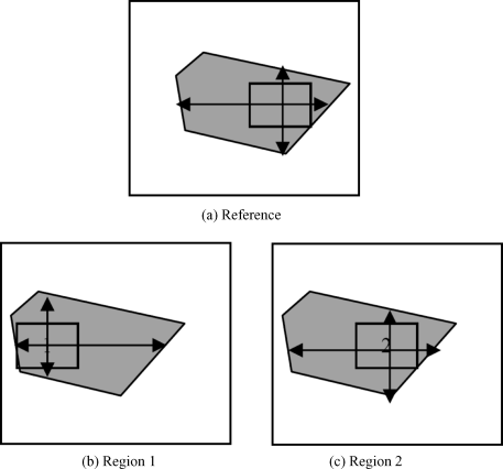
An alternative to the described treatment of untextured regions is to explore the distances of this region to the surrounding edges [17]. This will be explained by Figure 4.10 with untextured regions in gray and in the hatched areas. The essential feature of the search for the edges is the shifting of windows to the edges and the determination of the distances to the edges. This is shown in Figure 4.11a and b where the distances to the edges are indicated by arrows. This leads to a reformulation of Esmooth in Equation 4.8 into the following form [17]:
DL and DR are distances to the edges in the left and right eye images in various directions V as indicated in Figure 4.11a and b. The term SED is based on the sum of absolute edge differences (SED), while Equation 4.8 is based on differences of distances in x- and y-directions.
Figure 4.10 Image with untextured regions in the gray and hatched areas.
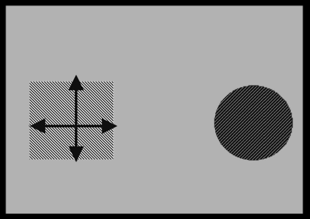
Figure 4.11 Search for distances to the edges in untextured regions.
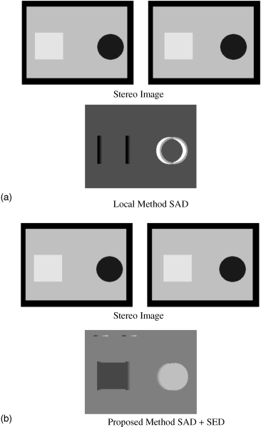
For an evaluation of the cost function Ed smooth, the disparity map for the image in Figure 4.10 is calculated. As the gray region but also the hatched square and the inside of the circle are untextured, the algorithm has to be applied for the gray region and for the interiors of the square and the circle. For the calculation of Edata in Equation 4.7 the SAD algorithm is used. The disparity map for SAD alone is depicted in Figure 4.12a underneath the original image, while Figure 4.12b shows the map obtained by SAD and SED. SAD alone leads to a false mapping, which is avoided by using SAD with SED.
Figure 4.12 Disparity maps for the untextured regions in Figure 4.10 obtained by SAD: (a) revealing false matches; (b) with SED resulting in correct matches.
4.4 An Algorithm Based on Subjective Measures
Physiologists have found that the HVS tries to understand the content of an image by detecting, comparing, and evaluating structural similarities, especially in proximate parts of the image. The algorithm based on these features is thus called the SSIM algorithm [3].
In this approach image degradations are estimated by the changes in the structural information perceived by the HVS. The parameters of an image providing this information will be the luminance of the individual pixels, the contrast created by the luminance of the pixels, and a comparison of the structural information. We assume the image is partitioned into spatial patches for a comparison of the properties of two selected patches. One patch has luminance xi in its pixels i and the second patch exhibits the luminance yi. Instead of spatial patches, other subdivisions can be imagined.
The mean luminance in the x-patch with N pixels is
(4.13)![]()
while the other patch similarly provides μy. For a comparison of μx to μy, the mean values are not that important. Therefore only the values xi − μx and yi − μy have to be considered. The functions l(x, y) for a comparison of luminance will depend on μx and μy.
The standard deviation σ, which is the square root of the variance, is used as a measure σx for the contrast with
As a justification for Equation 4.14 it is mentioned that the quadratic term is related to energy, which after applying the square root may be interpreted as contrast. The comparison of contrasts will depend on σx and σy.
Finally we consider the normalized signals x − μx and y − μy divided by their standard deviations, yielding
(4.15a)![]()
and
(4.15b)![]()
These signals have unit standard deviation; however, they differ otherwise. This difference is used in the comparison function S(x, y) for the structural differences in the two patches x and y.
The function S(x, y) for the comparison of the differences in the patches x and y is written as
Before we explain l(x, y), c(x, y), and s(x, y) and the function f, we want S(x, y) to satisfy the following conditions:
1. The symmetry S(x, y) = S(y, x), meaning that the similarity is independent of the denomination x or y of the patches.
2. Boundednes: S(x, y) ≤ 1, which is achieved by normalization.
3. Unique maximum: max S(x, y) = 1, if and only if x = y.
This means that only if the two patches are identical will we encounter the maximum similarity bounded by condition 1.
Now we define the three functions in Equation 4.16 such that conditions 1 to 3 are met.
We define the luminance comparison as
where C1 is introduced for the case of a very small ![]() which would lead to an unrealistically high luminance comparison. C1 is chosen as
which would lead to an unrealistically high luminance comparison. C1 is chosen as
(4.18)![]()
where L is the dynamic range of the gray scales, for example, 255 for an 8-bit word and ![]() .
.
Equation 4.17 meets the constraints 1 to 3 and is consistent with Weber's law which states that the HVS is sensitive to relative and not to absolute changes in luminance, meaning that at a high luminance only a larger change of it is perceived. This is the reason for the division with the total luminance.
The contrast comparison function c(x, y) assumes a form similar to Equation 4.17. It is
with C2 = (K2L)2 and ![]() . Again constraints 1 to 3 are met. With the same reasoning as for Equation 4.17, Equation 4.19 is consistent with the masking of the contrast by the HVS. This means that at a high contrast, only larger changes of it are noticeable.
. Again constraints 1 to 3 are met. With the same reasoning as for Equation 4.17, Equation 4.19 is consistent with the masking of the contrast by the HVS. This means that at a high contrast, only larger changes of it are noticeable.
Now we are ready to define the structure comparison function s(x, y). All the information about the two patches we have so far are the luminances x and y from which σx and σy in the luminance and contrast comparison functions l(x, y) and c(x, y) were derived. A measure on how the two structures are related to each other is offered by the cross-correlation function σxy which is used for the structure comparison function s(x, y) in the following form:
with the cross-correlation given as
(4.21)![]()
s(x, y) is again limited in value by the division with the product of the two mean luminances. C3 in Equation 4.20 avoids instability for very small values of σx and σy. Finally we have to combine the three comparison functions according to Equation 4.16 into the resulting SSIM index:
where α, β, γ > 0 are parameters used to adjust the individual weights of the three functions. Also, the SSIM index meets the three conditions 1 to 3.
For α = β = γ = 1 and C3 = C2/2, Equations 4.17, 4.19 and 4.20 yield with SSIM(x, y) in Equation 4.22
(4.23)![]()
For C1 = C2 = 0, SSIM was previously called the universal quality index (UQI) [18, 19].
Examples will now demonstrate how SSIM is able to assess the quality of images. The evaluation of an image is not just based on two patches which computer scientists call windows. The M windows covering the entire image to be assessed are created by shifting the two windows over the entire image. The mean of all these M images is given as
(4.24)![]()
In all examples a weighting function w = {wi}, i = 1, 2,. . ., N, for the N pixels in a window is used to obtain a locally isotropic quality map. The weighting changes μx, σx, and σxy into
(4.25a)![]()
(4.25b)![]()
and
(4.25c)![]()
The constants in the examples are always K1 = 0.01 and K2 = 0.03. Image quality assessment may degrade if different reference images and/or different distortions are encountered. We evaluate such cross-image and cross-distortion effects at the images in Figure. The figure captions to each image contain the subjective MSSIM indices. All MSE values are 210, so physically all images have the same distortion. The MSSIM values coincide much better with the subjective evaluation of the visual appearance. The mean-shifted image in Figure 4.13c is the most appealing and has the highest MSSIM value of 0.99, while the highest possible value is 1. Figure 4.13d and Figure 4.13e appear to be the worst, even though they have the same MSE as Figure 4.13c.
Figure 4.13 Six equal figures all with MSE = 210 but with different subjective image qualities: (a) original image with 8 bits per pixel; (b) contrast-stretched image MSSIM = 0.9168; (c) mean-shifted image MSSIM = 0.99; (d) JPEG compressed image MSSIM = 0.6949; (e) blurred image, MSSIM = 0.7052; (f) noise-contaminated image, MSSIM = 0.7748.
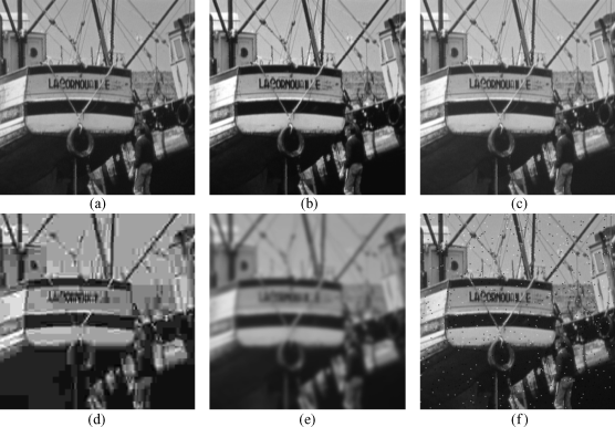
Figure 4.14a and Figure 4.14b show how the original image in Figure 4.14a is being distorted to Figure 4.14b by added noise. This can be improved by changing the MSSIM index along its steepest inclination, which is along the gradient of MSSIM(x, y), while constraining the MSE to remain equal. The equations for this procedure are
(4.26)![]()
(4.27)![]()
where:
σ is the square root of the constraint MSE.
λ defines the step size along the gradient.
P(X, Y) is a projection operator and Ê(X, Y) is a unit vector.
Figure 4.14 (a) Original figure; (b) figure with added noise; (c) noise-free figure with maximum MSSIM; (d) noise-free figure with minimum MSSIM, still impaired.
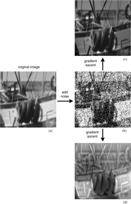
MSSIM is differentiable and converges to both a maximum of the MSSIM associated with a noise-free Figure 4.14c and a minimum MSSIM in Figure 4.14d associated with a noise-free but still impaired and distorted figure.
The given, not data-compressed images in Figure 4.15a–c undergo data compression according to JPEG and as a consequence the image quality usually suffers. The original images have a resolution of 24 bits per pixel. The compressed resolution, the PSNRs, and the MSSIMs of the compressed Figure 4.15d–f are listed in the figure captions. It is worth noting that at a low bit rate the coarse quantization of JPEG often results in a smoothed-out representation of the fine-detail regions in the image, as visible in the tiles in Figure 4.15d.
Figure 4.15 (a)–(c) Original images with 24 bits per pixel; (d) image compressed to 0.2673 bits per pixel with PSNR = 21.98 dB, MSSIM = 0.7118; (e) compressed to 0.298 bits per pixel with PSNR = 30.87 dB, MSSIM = 0.8886; (f) compressed to 0.7755 bits per pixel with PSNR = 36.78 dB, MSSIM = 0.9898; (g)–(i) SSIM maps of compressed images; (j)–(l) absolute error maps of compressed images with contrast inverted for easier comparison with SSIM maps.
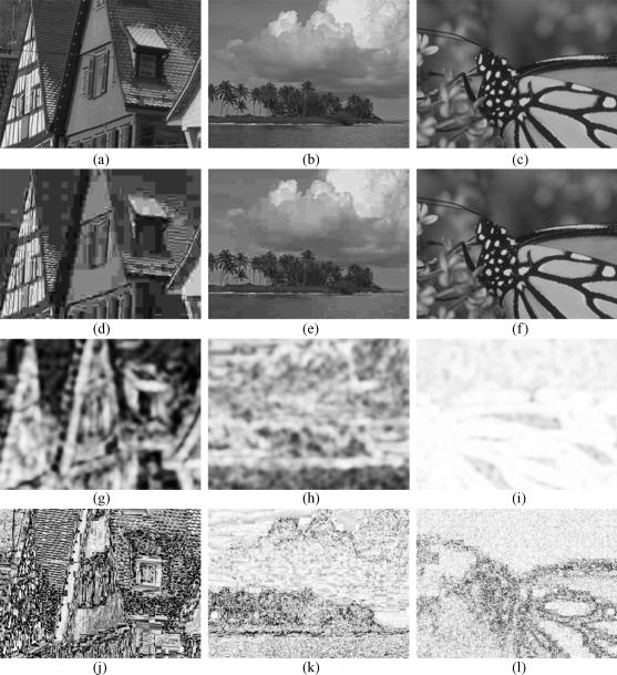
The images in Figure 4.15g–i represent a map for the local SSIM indices where brightness indicates the magnitude of SSIM. The images in Figure 4.15j–l show a map for the absolute error. The absolute error in Figure 4.15j in the region of the tiles looks no worse than in other regions, so the smoothing out is not noticeable at absolute errors. Figure 4.15g demonstrates that with SSIM these poor-quality regions are better captured than by the absolute error.
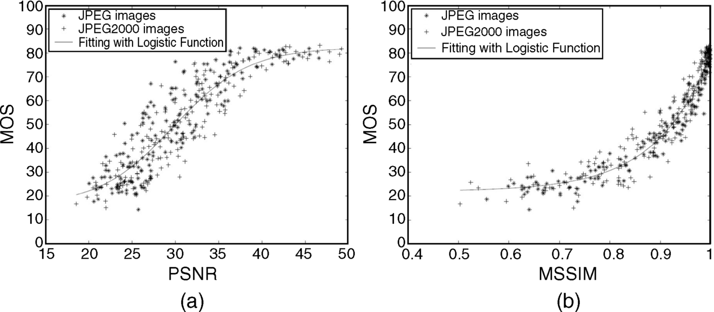
A group of test viewers provided mean opinion scores (MOSs) for the perceived quality of an image. These were applied to images after data compression by JPEG and JPEG 2000. The estimation of the image quality in MOS was performed for an increasing PSNR in Figure 4.16a and for an increasing SSIM index in Figure 4.16b. The full line is the fitting curve approximating the cloud of points. The points in Figure 4.14b are moved close to the fitting curve. This means that the viewers were able to predict the MSSIM rather closely. It also indicates that the subjective measure MSSIM is close to the subjective judgment of the viewers. This is not the case in Figure 4.16a where the points are scattered over a larger area around the fitting curve. The reason is that the subjective judgment of the viewers does not correlate well with the objective measure of PSNR.
Figure 4.16 The MOS of a JPEG image, and a JPEG 2000 image with a fitting curve (a) versus the PSNR, and (b) versus the MSSIM index.
So far the quality of an image has been evaluated from one fixed position of the viewers. As quality is affected by the viewing angle and to a lesser degree also by the distance of the viewer to the screen of the display, an extension of the SSIM measure to several viewing positions, also called scales, is required. This extension was denominated as a multiscale SSIM [4]. The single scale SSIM index in Equation (c04-mdis-0031) was reformulated as
(4.28)![]()
where j indicates one of the V different viewing positions. Hence the VSSIM is a quality measure including not only one scale, but also V scales of the image. The original image has the scale j = 1. At the highest scale j = V the luminance lV(x, y) is taken for all positions. A simplified parameter selection assumes αj = βj = γj for all the j and the normalization ![]() . This renders parameter settings for single scale and multiscale arrangements comparable. The remaining task is to determine the various functions lV, cj, and sj where the CSF of the HVS [20] plays a role. It states that the visual contrast sensitivity function peaks at medium spatial frequencies of 4 cycles per degree.
. This renders parameter settings for single scale and multiscale arrangements comparable. The remaining task is to determine the various functions lV, cj, and sj where the CSF of the HVS [20] plays a role. It states that the visual contrast sensitivity function peaks at medium spatial frequencies of 4 cycles per degree.
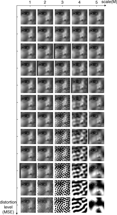
In order to calibrate the relative importance of the different scales a synthesis and analysis are performed as depicted in Figure 4.17. The first row shows the original image for five different scales. Each image is distorted by MSE increasing in each column in the downward direction. The distortion is created by adding white Gaussian noise. The distortions at different scales are of different importance for the perceived image quality. Images in the same row have the same MSE. The test persons identified one image in each column with the same quality. This should demonstrate how well the multiscale approach works. One set of equal-quality images is marked by frames. This reveals that at different scales (columns), different distortions are needed in order to generate the same image quality. Scale 1 allows for the largest distortions and scale 3 is more sensitive and tolerates only a minimum of distortions for the same subjective image quality.
Figure 4.17 Images seen from five viewing directions (scales) with increasing MSE downward in the columns.
The examples for single and multiscale SSIM confirm that the SSIM index is able to match the subjective assessment of quality of the HVS. The steepest ascent along the SSIM is a powerful means for enhancing image quality. As distortions affect image quality differently in different viewing directions (scales), the designer of a 3D system can detect where special care for quality has to be applied. Both single and multiscale features are important for the development of high-quality 3D displays for TV, computers, mobile phones, medical and educational imaging, and advertising as well as for 3D TV.
4.5 The Kanade–Lucas–Toman (KLT) Feature Tracking Algorithm
The algorithm tracking the time-dependent path of a selected feature in a frame-wise sequence of images provides a motion vector and the associated disparity of the path [18, 22–25]. In many cases the feature is based on an intensity I(x, y, t) dependent on the spatial coordinates x and y of the image and the time t. The property of such an intensity feature is given by
(4.29)![]()
meaning that the feature taken at the time t + τ is the same as the feature taken at the time t shifted by ξ in the x-direction and by η in the y-direction. The vector of the motion is
with the components ξ and η. ![]() is also called the displacement. We first consider the one-dimensional case where the feature at the beginning of the tracking is G(x) and the shifted feature is F(x) [22, 23]. For a small shift
is also called the displacement. We first consider the one-dimensional case where the feature at the beginning of the tracking is G(x) and the shifted feature is F(x) [22, 23]. For a small shift ![]() = ξ the shifted feature can be approximated by
= ξ the shifted feature can be approximated by
(4.31)![]()
The difference between G(x) and F(x + ξ) defined by an error E is in the L2-norm
E is summed for all values of x or pixels in the window around the selected feature. One could minimize E by searching for a set of x- and ξ-values as was done for the SAD algorithm in Equation 4.4. This leads to a heavy load of calculations. Therefore, in this case a computationally less demanding approach was chosen.
The minimization of E with respect to ξ provides [22]
![]()
or
yielding
It can be assumed that F′(x) ≠ 0 for at least one x; ξ has to meet the condition of convergence F(x + ξ) → G(x), which can only be determined for given functions G(x). The obvious rule is ξ must be small enough. For G(x) = sin x it can be shown that |ξ| < π is required.
In a display working with a frame time Tf the magnitude of the motion vector ![]() = (ξ, η) is determined in the one-dimensional case by ξ = vxTf, where vx is the velocity of the object in the x-direction. A small frame time Tf of, for example, 4.16 ms for a 240 Hz frame used for suppressing blur or for time-multiplexed autostereoscopic displays is certainly also helpful for limiting ξ and so is a small velocity vx.
= (ξ, η) is determined in the one-dimensional case by ξ = vxTf, where vx is the velocity of the object in the x-direction. A small frame time Tf of, for example, 4.16 ms for a 240 Hz frame used for suppressing blur or for time-multiplexed autostereoscopic displays is certainly also helpful for limiting ξ and so is a small velocity vx.
The calculations leading to ξ in Equation 4.33b have to be repeated from frame to frame yielding the iteration
(4.34)
where also a weighting function w(x) has been assigned to F(x) and G(x).
For an extension to multiple dimensions we consider x to be a row vector ![]() (x1, x2,. . ., xn) with components x1 to xn. As a rule in displays we have two components x1 and x2 = y for the two-dimensional screen.
(x1, x2,. . ., xn) with components x1 to xn. As a rule in displays we have two components x1 and x2 = y for the two-dimensional screen.
Then
![]()
is a vector transposed into a column vector with the partial derivatives ∂/∂xν.
With these denominations and the now also multidimensional displacement ![]() in Equation 4.30, Equation 4.33a becomes
in Equation 4.30, Equation 4.33a becomes
(4.35a)![]()
resulting in
So far we have assumed that the transition from ![]() to
to ![]() is a single translation vector
is a single translation vector ![]() = (ξ, η) in the two-dimensional case. This is extended to an arbitrary linear transformation such as a rotation, scaling, and shearing. This transformation can be expressed by a new, more general displacement [23, 24]
= (ξ, η) in the two-dimensional case. This is extended to an arbitrary linear transformation such as a rotation, scaling, and shearing. This transformation can be expressed by a new, more general displacement [23, 24]
(4.36)![]()
where
is the translation matrix and ![]() is the known displacement, in this case of the center of the window around the feature selected. The translation matrix D can also describe an affine motion field of feature in its window, where each point x exhibits a different motion forming a field of motions.
is the known displacement, in this case of the center of the window around the feature selected. The translation matrix D can also describe an affine motion field of feature in its window, where each point x exhibits a different motion forming a field of motions.
If the intensities and the contrasts in the two images G(x) and F(x) differ due to different viewpoints, we can account for this by assuming G(x) to be the updated form
(4.38)![]()
This finally yields E similar to Equation 4.32 as
(4.39)![]()
With the linear approximation
(4.40)![]()
one can calculate according to Equations 4.33b the minimization of E and the displacement of ![]() providing the four parameters in the matrix D in Equation 4.37 and the two components ξ and η of
providing the four parameters in the matrix D in Equation 4.37 and the two components ξ and η of ![]() in Equation 4.30. Further details can be found in [23, 24].
in Equation 4.30. Further details can be found in [23, 24].
For the selection of appropriate features for tracking, one can focus on corners, highly textured regions which contain high spatial frequencies, or on areas with sufficiently high second-order derivatives. A more analytical approach [24] is to require that the term
![]()
containing the gradient of the selected feature is large enough to exceed the noise level. This ensures that both eigenvalues λ1 and λ2 of the 2 × 2 matrix for ![]() exceed a given level λ, meaning that
exceed a given level λ, meaning that
(4.41)![]()
where λ is a predetermined threshold.
For the determination of λ we note that a region untextured or weakly textured with a roughly uniform luminance does not provide any useful features. The eigenvalues of the gradient-related matrix are therefore very small and are as a rule exceeded by noise. So the eigenvalues should exceed these low gradients. The eigenvalues of the gradient in three typical regions are depicted in Figure [25]. For the completely untextured region in Figure 4.18a they are zero, indicating rank 0 of the pertinent matrix; the more the regions are textured in Figure 4.18b and 4.18c, the larger are the eigenvalues and the ranks. So the lower bound for λ corresponds to the weakly textured region and the upper bound is derived from highly textured regions or corners. The recommendation for the selection of λ is half way between the two bounds.
Figure 4.18 Different degrees of texture: (a) untextured region, λ1 = λ2 = 0, rank 0 of matrix; (b) weakly textured region λ1 > λ2 = 0, rank 1 of matrix; (c) highly textured region, λ1 > λ2 > 0, rank 2 of matrix. (Carnegie-Mellon University report [25]).
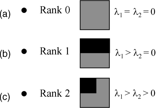
An experimental example demonstrates the feature selection and properties of tracking [23]. Figure 4.19a shows a set of features at the beginning of the tracking procedure, while Figure 4.19b depicts the surviving features at the end of the tracking after a total displacement of about 100 pixels, which is one pixel per frame. The eigenvalues of the gradient matrix at the beginning of the tracking are shown in Figure 4.20a where brighter areas mean larger eigenvalues. The man in the traffic sign and the texture of the mug provide the largest eigenvalues, while the artichoke and the teddy bear are lower, but still noticeably textured. Figure 4.20b depicts the surviving eigenvalues at the end of the tracking after 100 frames; 216 of 226 selected features survived the tracking. The surviving features are indicated by squares. In each tracking step corresponding to the investigated frames, at most five iterations were needed for the matching.
Figure 4.19 (a) Features in an image at the beginning of the tracking and (b) surviving features at the end of tracking after 100 frames with a total displacement of 100 pixels. (Carnegie-Mellon University report [23]).
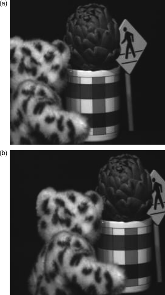
Figure 4.20 (a) Map of eigenvalues at the beginning of tracking; brighter areas mean larger eigenvalues. (b) Map of eigenvalues at the end of tracking after 100 frames. (Carnegie-Mellon University report [23]).
The tracking algorithm has an important application in 3D technology. From the vector of motion ![]() and from the two pertinent images taken from the moving object at different times, a 3D effect is derived according to the Pulfrich phenomenon [26]. In this effect one eye is covered by a dark filter. The eye and the brain require additional time to process the dark image. Hence the perception of the dark image is delayed toward the perception of the bright image received by the other eye. This delay generates the sensation of depth. This effect is used for creating 3D images from the two images, one delayed with respect to the other. The two images are called the right eye and the left eye image. The Pulfrich effect works even better when the two images are not the same, as is the case for the tracking of a feature. Here the later image is seen from a different viewpoint which renders the image of the same object slightly different, called motion parallax.
and from the two pertinent images taken from the moving object at different times, a 3D effect is derived according to the Pulfrich phenomenon [26]. In this effect one eye is covered by a dark filter. The eye and the brain require additional time to process the dark image. Hence the perception of the dark image is delayed toward the perception of the bright image received by the other eye. This delay generates the sensation of depth. This effect is used for creating 3D images from the two images, one delayed with respect to the other. The two images are called the right eye and the left eye image. The Pulfrich effect works even better when the two images are not the same, as is the case for the tracking of a feature. Here the later image is seen from a different viewpoint which renders the image of the same object slightly different, called motion parallax.
It is now clear that the KLT tracking algorithm plays an eminent role in the endeavor of generating 3D images.
4.6 Special Approaches for 2D to 3D Conversion
The algorithms in Sections 4.1–4.5 mainly dealt with the extraction of disparity or depth from given right eye and left eye views of a 3D display. This could also be used to obtain the depth inherent in a 2D display if a second view as a reference image were available. However, if one wants to deal only with the monoscopic 2D display a different approach is needed. This approach is based on physiological and physical depth cues in the 2D display such as luminance, contrast, sharpness, chrominance, horizontal motion, and depth from motion parallax (DMP). How luminance and contrast are related to depth perception has already been investigated in Section 3.5.
The availability of a depth map for a 2D display or to one of the two images required for a 3D display has the advantages for broadcasting that we already detailed at the end of Section 4.1. In the next section we shall have a look at the early, but very instructive, approaches for DIBR as a preparation for the final section in which the state of the art of DIBR will be presented.
4.6.1 Conversion of 2D to 3D images based on motion parallax
We shall now discuss some early approaches to extract disparity information from a 2D image and use it for the construction of a 3D image. The description of these approaches is intended to familiarize us with physiological depth cues, such as, for example, cues based on the Pulfrich effect presented at the end of Section 4.5. This effect is associated with motion parallax as used in [27].
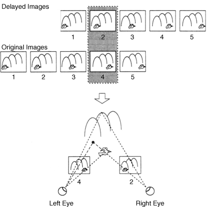
Figure 4.21 with five temporal sequences shows a bird flying to the right in front of mountains as the original images and, above, the same images delayed by two time slots. The original image in time slot 4 is chosen as the left eye image and the delayed image in time slot 2 as the right eye image as depicted below. The eyes are rotated until their axes intersect at the present location of the bird. This is the situation in Figure 1.1, where the eyes focus on point Q and the rotation occurs by the angles γ1 and γ2 for the left and the right eye respectively. The difference of these angles is the disparity indicating the depth. So the locations of the bird provide a sensation of depth. However, this is an illusionary depth because the speed of the bird has no relation at all to its depth. This is further elucidated by the next observation. If the bird flies slower it would be located further to left in Figure 4.21 as indicated by the dashed line from the left eye, while the starting position for the right eye remains the same. In this case the intersection of the axes of the eyes is of course further to the left but also higher up closer to the mountains. This indicates a larger depth even though the bird has the same depth as before. This again is an illusionary depth, which we have to cope with in the next section. In the present case it requires a correction that we do not have to deal with now. This method of depth generation in [27] is based on a so-called modified time difference (MTD).
Figure 4.21 Determination of the left and right eye images from a 2D object moving to the right.
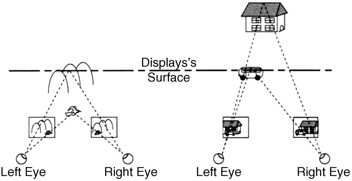
If the object, such as the car in Figure 4.22, moves in the opposite direction to the left, the axis of the left eye is directed toward the earlier position of the car, while the axis of the right eye follows the car to its later position. This is the reverse of the movement to the right. Also, here a correction according to the speed of the car has to be done.
Figure 4.22 Determination of the left and right eye images from a 2D object moving to the left.
The above described activities of the eyes serve only to explain the construction of the left and right eye images for the successful generation of 3D images. It is not assumed that the eyes react that way in reality.
Signal processing for the MTD process is shown in Figure 4.23. The ADC provides the digital form of the analog signal, which is again converted back to analog form by the DAC at the output. The movement detector provides the direction and the speed of the movement, whereas the delay time controller provides the speed-dependent correction of the depth. The delay direction controller guides the starting position to the right eye for a movement to the right and to the left eye for a movement to the left.
Figure 4.23 Block diagram for the 2D/3D conversion according to the MTD process.
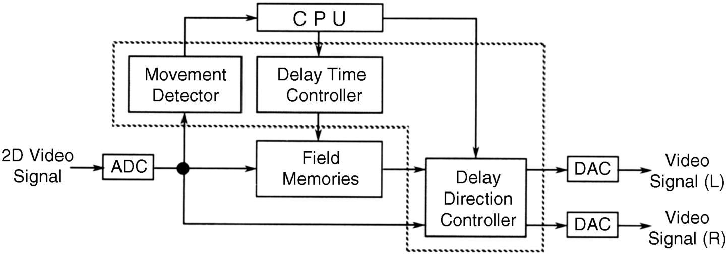
The chip required for the processing works in real time on the incoming 2D images.
4.6.2 Conversion from 2D to 3D based on depth cues in still pictures
The MTD method works only for moving objects. For still images it has to include a disparity extraction based on contrast, sharpness, and chrominance. Contrast and sharpness are associated with luminance. Sharpness correlates with high spatial frequencies, while contrast is related to medium spatial frequencies. Chrominance is associated with the hue and the tint of the color. The approach based on these features is called the computed image depth (CID) method [28, 29].
Near objects exhibit a higher contrast and a higher sharpness than objects positioned farther away. So contrast and sharpness are inversely proportional to depth. Adjacent areas exhibit close chrominance values, thus indicating that they have the same depth. Chrominance is a measure for the composition of the 2D image. The features contrast, sharpness, and chrominance allow the depth classification far–mid–near as depicted in Figure 4.24.
Figure 4.24 Determination process for classification of depth as near–middle–far based on contrast, sharpness, and composition.
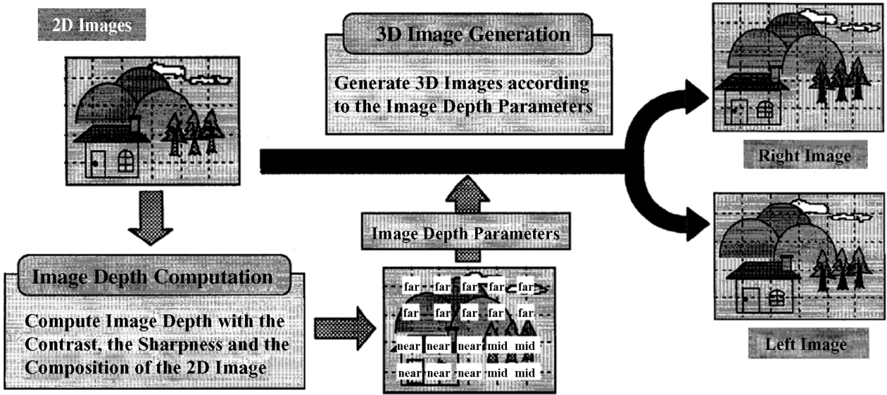
Finally, if the classification is “near,” the left eye image is created by shifting the image investigated to the right and the right eye image by shifting to the left corresponding to the crossed disparities. If the classification is “far,” both the right and the left eye images are created by shifting the image in the opposite directions of the near case as for uncrossed disparities. This is depicted at the output of Figure 4.24.
This CID method provided the depth map in Figure 4.25b pertaining to the image in Figure 4.25a. The MTD and CID methods are combined in [28, 29].
Figure 4.25 The given image in (a) and the pertinent depth map in (b).
4.6.3 Conversion from 2D to 3D based on gray shade and luminance setting
In [30] three attractive and successful features for the determination of depth in 2D images are investigated: namely, gray-scale analysis, relative spatial setting, and multiview 3D rendering.
A color image is simply converted into one intensity value I with a gray scale
(4.42)![]()
where the right side contains the intensities of the colors. In Figure 4.26 and in the block diagram in Figure 4.27 this is called gray-scale conversion. The gray scale I is expanded into I′ with a range from 255 to 0 for an 8-bit word by the equation
(4.43)![]()
Figure 4.26 The gray-scale conversions of a figure.
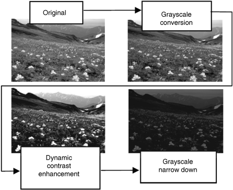
Figure 4.27 Block diagram for gray-scale conversions.
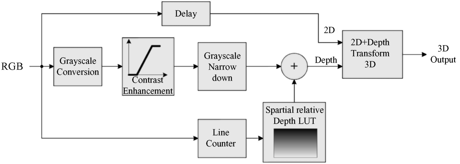
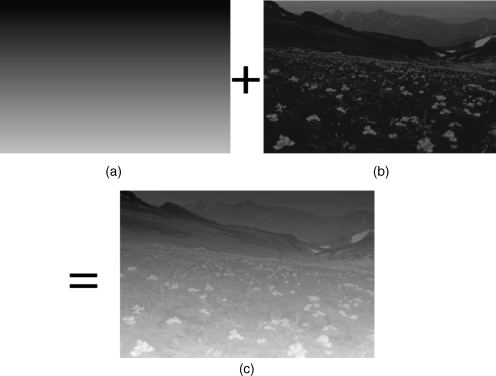
This is called the dynamic contrast enhancement, which is followed by a narrowing down of the gray scale to the range 0–63. Figure 4.26 shows the appearance of the image after these individual steps. In the next step the luminance of the entire image is reset by assigning a smaller luminance to the upper portion which is gradually getting brighter toward the lower portion, as depicted in Figure 4.28a–c. After application of the setting, the image with the increasing gray scale toward the bottom in Figure 4.28c conveys a very impressive sensation of depth (even though the reproduction quality of the figure may be low). This reminds us of another depth-enhancing cue in brighter images, which is rendering objects slightly more bluish the farther away they are.
Figure 4.28 (a–c) Resetting of luminance for enhancement of depth with final result in (c).
Counteracting this depth enhancement is a spot at any depth reflecting light, like the human eye in Figure 4.29a reflecting a beam of light. This effect induces the sensation of a shorter depth. A 1D median smooth filter [31] is used to suppress this effect.
Figure 4.29 The reflection in an eye (a) and its removal by a 1D median filter in (b).
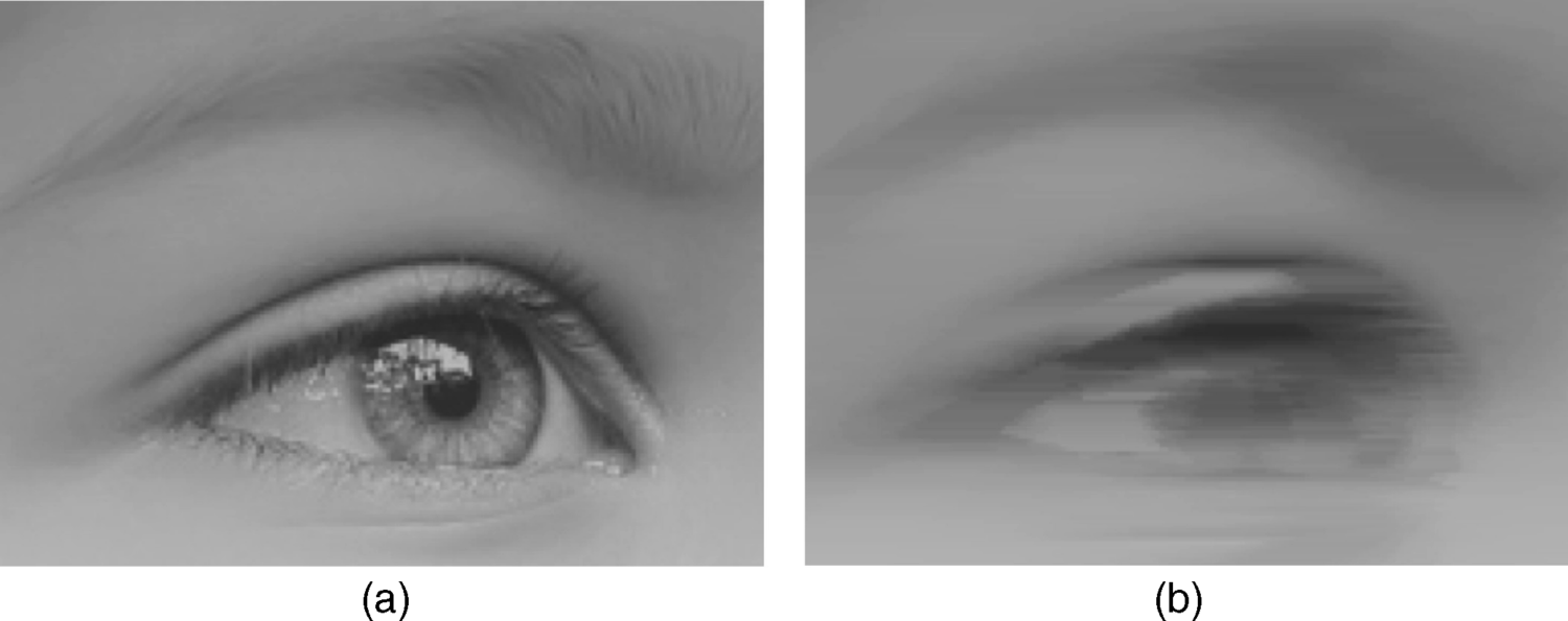
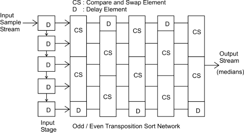
We shall take a brief look at the operation of a 1D median filter as shown in Figure 4.30. Five samples, pixels in our case, representing a window in the input sample stream, are shifted toward the output through five stages performing a compare-and-swap operation. This means in our case that the luminances are successively compared and ordered in a sequence of diminishing luminances. The third luminance is the median. The top value is discarded. After this filtering the eye looks free of reflection as depicted in Figure 4.29b.
Figure 4.30 Operation of a 1D median filter.
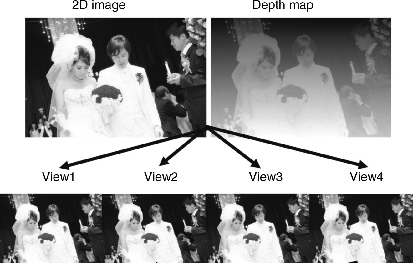
The last step is multiview rendering for a presentation through a slanted array of lenticular lenses. We have investigated the pixel arrangement for this type of lenticular lens in Section 3.1 and Figures 3.7, 3.10, 3.12, 3.18 and 3.20 which for multiple views had to correspond to the projection angle ϕ of a lens in Figure 3.8. The same pixel arrangement for four views is also applied in the present case and is shown in Figure 4.31. The four views are paired into two views according to different depths assigned to each pair as provided by the depth map. For the image on the left in Figure 4.31 the depth map is shown in Figure 4.32 on the right with brighter areas for a smaller depth. The four viewing directions are shown in the second line.
Figure 4.31 The pixel arrangement for four different views.
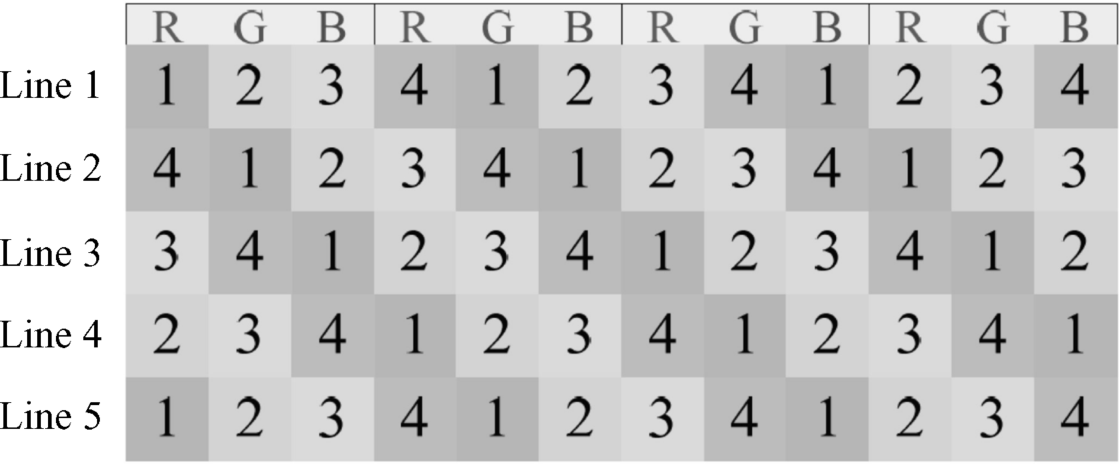
Figure 4.32 The 2D image and its depth map in the upper line. The four views for Figure 4.31 are in the lower line.
This 2D/3D conversion does not require a complex motion analysis.
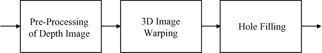
4.7 Reconstruction of 3D Images from Disparity Maps Pertaining to Monoscopic 2D or 3D Originals
DIBR requires two monoscopic images for the reconstruction of 3D images. They are the 2D picture or one of the left or right eye images needed for 3D perception and the pertinent depth or disparity map [32–35]. The three processing steps resulting in a 3D image are shown in the block diagram in Figure 4.33 [33].
Figure 4.33 Block diagram for the processing required to obtain a 3D TV image.
4.7.1 Preprocessing of the Depth Map
The first task is to determine the maximum and minimum disparities Dmax and Dmin in a disparity or depth map. This is later required for the generation of the left and the right eye images.
For use in a computer program, a shift and a normalization of the disparities D may be helpful. The shift is performed by a center value
(4.44)![]()
For an 8-bit disparity value Dnear = 255 and Dfar = 0. The normalized and shifted Dn is
(4.45)![]()
The quality of a depth map as a rule needs some improvements. Most frequently used is the smoothing of the values in the depth map d(x, y) in the spatial x, y domain by a Gaussian filter with the filter function in the x-direction of the spatial domain
(4.46)![]()
σx is the standard deviation and w stands for the size of the window in which the filter is applied. Filtering in the y-direction has the same form with y and σy. The σ-values determine the strength of the filter. After filtering d(x, y) has assumed the form of a smoothed depth map
Often w = 3σ is chosen. In Equation 4.47 the σ-values depend on μ and υ; more often they are the constants σx and σy.
As we already know, the Gaussian filter results in the suppression of noise and the smoothing of sharp edges and abrupt discontinuities.
The HVS obtains depth cues mainly from differences of disparity along the horizontal axes rather than from the vertical differences. This allows the depth map in the vertical direction to be filtered more strongly than in the horizontal direction. This freedom in the selection of the σ-values can satisfy the need for a sharp removal of noise, while still causing the least distortion of the depth cues in the horizontal direction. In an example with σx = 10 and σy = 90, which is called asymmetric filtering, the effect on the reconstructed 3D image will be demonstrated and compared to the symmetric filtering with σx = σy = 30 [33]. Figure 4.34a shows a 2D image, the interview, with its unprocessed depth map in Figure 4.34b. The images in Figure 4.35a and 4.35b depict the depth map after symmetric and asymmetric smoothing. After some more processing steps to be discussed below, we obtain the two left eye images for a 3D display in Figure 4.36a for symmetric and in Figure 4.36b for asymmetric smoothing. The curved leg of the table in Figure 4.36a, shown enlarged in Figure 4.16a, demonstrates that symmetric smoothing causes geometric distortions in the vertical direction which do not occur for asymmetric smoothing in Figure 4.36b. For an explanation we note that the depth of the leg in the vertical direction is, according to Figure 4.34b, everywhere the same. After symmetric smoothing of the depth map with a more heavy impact due to a large σ-value also in the horizontal direction, the shape of the leg due to smoothing becomes wider at the bottom, causing the curved appearance. This is not the case for asymmetric smoothing as the impact of smoothing due to a smaller σ-value in the horizontal direction does not exhibit this widening effect.
Figure 4.34 The 2D image, the interview in (a), and its unprocessed depth map in (b).
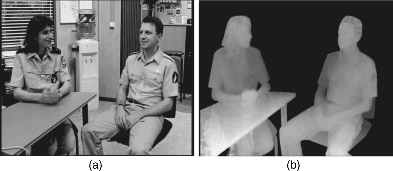
Figure 4.35 The depth map in Figure 4.34b (a) after symmetric smoothing and (b) after asymmetric smoothing.
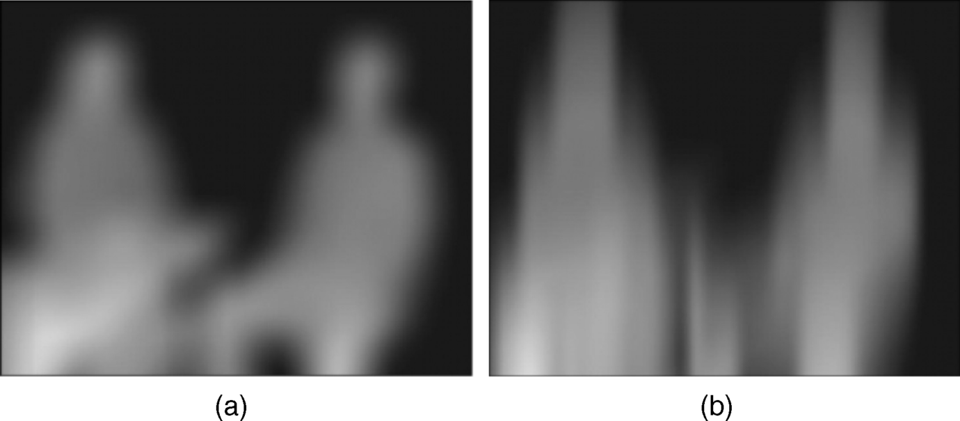
Figure 4.36 (a–c) Left eye image in Figure 4.34a (a) after symmetric smoothing (b) after asymmetric smoothing and (c) Enlarged curved leg in Figure 4.36a.
4.7.2 Warping of the Image Creating the Left and the Right Eye Views
Warping is the method used to generate the left and the right images for 3D perception. It is different if a depth map is involved or if the motion vector in motion parallax is used [33].
For the depth map approach we start with Figure 4.1 where the points el and er designate the location on the LCD screen of the left and right eye images of the object Q. In the left eye, the object Q is seen at an angle α and in the right eye at an angle β. The images are shifted by a distance fb/2z from the intermediate image at em to the right and to the left according to Equations 4.1e,f, repeated here respectively:
![]()
To generate the left and right eye images we take the intermediate image at em from the 2D picture and assign to it the depth z from the depth map at the point em. The depth z is needed in Equations 4.1e,f.
For autostereoscopic displays which have lenticular lenses in front of the LCD screen, we encounter exactly the situation in Figure 4.1. So b is the interocular distance and f is the focal length of the lenses. Now the values of the shift in Equations 4.1e,f are known and we shift the intermediate image by fb/2z to the left and to the right thus creating the left and right eye images.
In the case of stereoscopic displays which require glasses, the figure corresponding to Figure 4.1 is Figure 4.37. There the points cl and cr indicate the cameras with focal length f, while from point cc we have the center or intermediate view to object P. The distance tx between the cameras, called the baseline distance, corresponds to b in Equations 4.1e,f. The depth z of the intermediate image at cc is again taken from the depth map. With these values the shifts into the right and left eye images are also known for stereoscopic displays.
Figure 4.37 Cameras with focal length f at the locations cl and cr generating stereoscopic images at depth z.
Equations 4.1e,f can also be derived from Figure 4.37. As an example for stereoscopic displays [33], the given 2D image and its depth map in Figure 4.38a and b are warped into a 3D image with the left image being shown in Figure 4.39. This figure enables a judgment on how the left eye image improves, from top to bottom, from no smoothing to symmetric and finally to asymmetric smoothing. The baseline distance in these figures was 36 pixels.
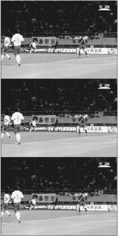
Figure 4.38 The soccer scene (a) and its depth map (b).
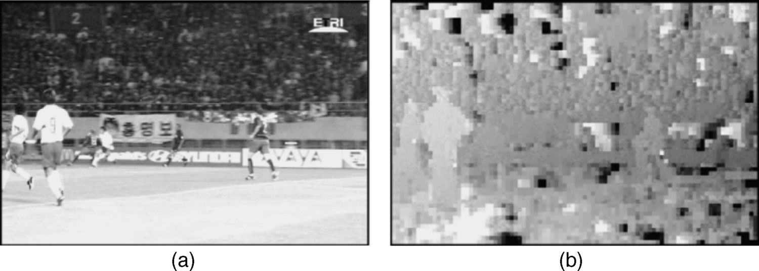
Figure 4.39 The left eye image in Figure 4.38 with no depth smoothing, symmetric smoothing, and at the bottom asymmetric smoothing.
For 3D images based on the vector ![]() of motion in Equation 4.35b obtained by the feature tracking algorithm, the determination of the left and right eye images is slightly more involved [34]. The reason is, as mentioned at the end of Section 4.6, that the vector of motion with the speed and its direction has no relation at all to the depth required for the reconstruction of 3D images. We could try to take the depth of the feature at the beginning of the tracking, which may change during tracking. If the object chosen as the feature exhibits a variety of depths, one could choose an average depth. In cases where this is too inaccurate, a different depth search has to be applied. In [34] such a search is based on three depth cues: magnitude of the motion vector, camera movements, and scene complexity. From Section 4.6 we know that the assignment of a picture to the left and to the right eye depends on the direction of the motion to the right or to the left. The motion vector
of motion in Equation 4.35b obtained by the feature tracking algorithm, the determination of the left and right eye images is slightly more involved [34]. The reason is, as mentioned at the end of Section 4.6, that the vector of motion with the speed and its direction has no relation at all to the depth required for the reconstruction of 3D images. We could try to take the depth of the feature at the beginning of the tracking, which may change during tracking. If the object chosen as the feature exhibits a variety of depths, one could choose an average depth. In cases where this is too inaccurate, a different depth search has to be applied. In [34] such a search is based on three depth cues: magnitude of the motion vector, camera movements, and scene complexity. From Section 4.6 we know that the assignment of a picture to the left and to the right eye depends on the direction of the motion to the right or to the left. The motion vector ![]() is provided by the algorithm in Section 4.5.
is provided by the algorithm in Section 4.5.
The conversion of the motion vector into disparity in [34] as a measure of depth starts with the determination of the maximum and minimum disparity DmaxO and DminO in a sequence of images. The maximum disparity for the motion-to-disparity conversion using the three cues above is
where Ddisplay represents the maximum disparity allowed by the characteristics of the display. The scaling factors stemming from the three cues of magnitude of motion, movement of camera, and complexity are now explained. The values of the cues are chosen very intuitively, as is the entire procedure.
Cue 1 is proportional to the maximum Mmax defined as the mean of the upper 10% of the magnitudes of the motion vectors in an image. This is contained in
(4.49)![]()
where the search range for motion is the interval of the values in which the search for magnitudes was executed. The normalization by the search range guarantees that cue 1/α1 ≤ 1, where α1 is a weighting factor.
Cue 2 relates to camera movement, which can distort the motions in an image. The background of an image without motion starts moving and the important motion in cue 2 relates to the camera movement and its distortion of the motions in the image. The foreground is falsified. This effect is also compensated in the MPEG algorithm for data compression [36]. The most disturbing movements of the camera are panning and zooming. In order to diminish the influence of these movements, cue 2 in these cases should exhibit a smaller value for the disparity leading to the factor (1 − cue 2) in Equation 4.48. Cue 2 has the form
(4.50)![]()
The panning and zooming are determined in blocks of the image in Figure 4.40a and 4.40b. Block panning is the magnitude of the unidirectional motion in a block, while block zooming is the outward-oriented magnitude of the zooming motion. These values are preferentially measured in an area of the background supposed to be stationary. The values are normalized by the pertinent areas guaranteeing that cue 2/α2 ≤ 1, where α2 is a weighting factor.
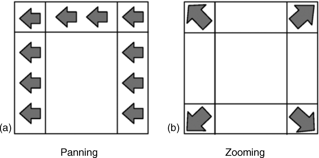
Figure 4.40 A block with (a) panning and (b) zooming of the camera.
Finally, cue 3 corresponds to the complexity of motion in various blocks of the image, especially when the difference between the motions in the current block investigated and previous blocks is large. It is impossible to assign a meaningful disparity to a block with a large number of motion vectors or a large difference in magnitudes of motion to previous blocks. Therefore the term complex block was introduced, which represents the number of blocks in an image where the difference of motion magnitudes between the current and the previous block exceeds a given threshold. This leads to
(4.51)![]()
Division by the total number of blocks guarantees that cue 3/α3 ≤ 1, where α3 is a weighting factor.
Block complexity is detrimental for a correct estimation of disparity and has therefore a limiting influence expressed by the factor (1 − cue 3) in Equation 4.48.
For the generation of the two images needed for 3D one has to determine by how much in cm or by how many pixels the two images have to be separated from the center image. For a width of 0.032 cm per pixel the relation between centimeters and pixels is
![]()
The necessary fusion of the two images only occurs if the shift between them, that is, the disparity, is neither too small nor too large. An experiment on this topic provided Table 4.1[34] in which the disparity is listed in cm together with a “o” indicating a successful fusion and a “×” for no fusion. This is a very interesting experiment. It does not reveal what the correct disparity is but at which disparities fusion is enabled. We encountered this in Section 4.6.1, with Figure 4.20, where the two images were 100 frames, apart. With the locations in Table 4.1 the occurrence of fusion was found experimentally. However, Equation 4.48 offers additional information on depth and disparity, namely, the maximum disparity Dmax depending on the depth cues of individual regions in the display. At the beginning of warping the range of measured disparities of the given image was determined as DmaxO and DminO. So the maximum of all disparities provided by Equation 4.48 have to be fitted into this range, that is,
which can be achieved by selection of the weights α1, α2, and α3.
Table 4.1 Depth fusion for various disparity values.
| Test sets | Disparity (cm) | Depth fusion |
| 1 | 2.64 | × |
| 2 | 2.11 | × |
| 3 | 1.58 | × |
| 4 | 1.06 | o |
| 5 | 0.53 | o |
| 6 | 0.00 | o |
| 7 | −0.53 | o |
| 8 | −1.06 | × |
| 9 | −1.58 | × |
| 10 | −2.11 | × |
| 11 | −2.64 | × |
Equation 4.48 is sorting blocks in a given image according to a list of decreasing disparity-related measures. The fitting of these measures into the range of given true disparities of the image establishes the link between the related hypothetical measures and the true measures.
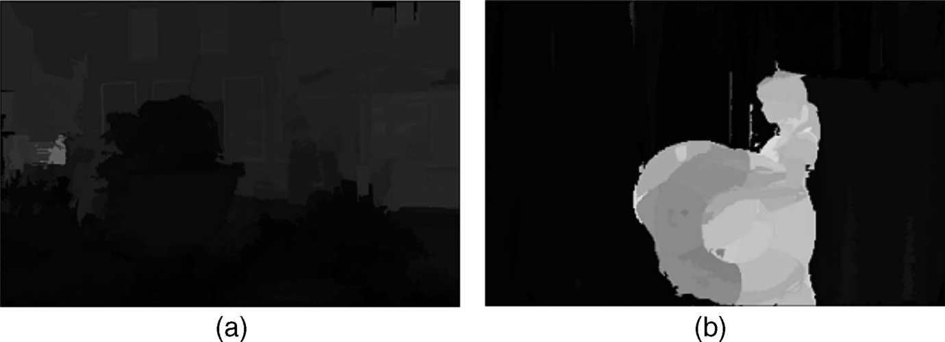
Depicted in Figure 4.41 are (a) a flower pot with people, a mostly still picture, and (b) a dancer dominated by motions. The dancer was captured with a fixed camera while the flower pot was captured with a fixed and panning camera. Figure 4.42a and 4.42b demonstrates the performance of the disparity estimation in Equation 4.48. In Figure 4.42a the motion of the only moving object in Figure 4.41a, a person, was detected as a small white area. In Figure 4.42b the strong motion of the dancer, shown in white, is visible, whereas the slower motion of the rings in the dancer's hand are caught as slightly darker areas.
Figure 4.41 (a) A flower pot with people, a predominantly still picture, captured with a fixed and a panning camera. (b) A dancer in motion, captured with a fixed camera.
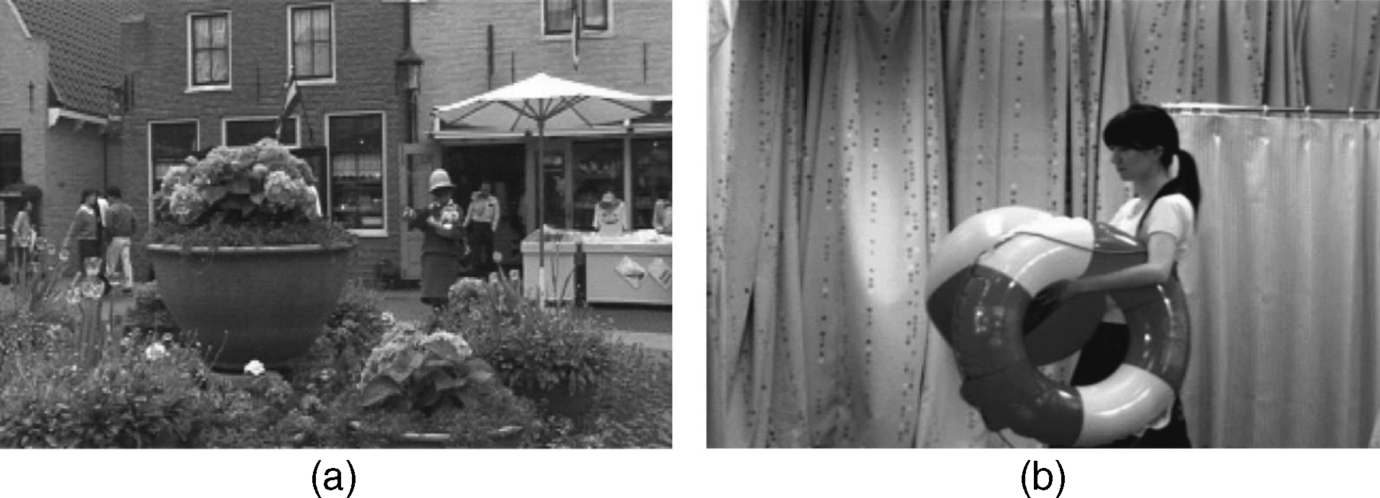
Figure 4.42 (a) Motion estimation of Figure 4.41a and (b) motion estimation of Figure 4.41b.
The diagrams in Figure depict the contributions of the three cues – the magnitude of motion in (a), the motion of the camera in (b), and the complexity of motion in (c) – versus the frames of the pictures. The dancer in Figure 4.43a contributes, as expected, much more to magnitude than the flower pot; in Figure 4.43b the panning camera contributes more to the flower pot than to the dancer; the complexity in Figure 4.43c of both the dancer and the flower pot tends with larger numbers of frames to equal contributions.
Figure 4.43 Contribution to the motion estimate in the “flower pot” and “dancer” images originating from (a) the magnitude of motion, (b) motion of the camera, and (c) the complexity of motion.
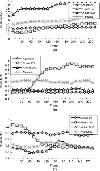
The examples show that the cues are able to classify motions.
4.7.3 Disocclusions and Hole-Filling
Occluded areas might become disoccluded in later images due to a different viewpoint in the left and the right eye obtained by warping. These areas have not yet received new information and hence do not exhibit a texture. They appear as a hole. There is no information about the hole in the center image or in the two eye images or in the depth map. The task is to fill the disturbing holes.
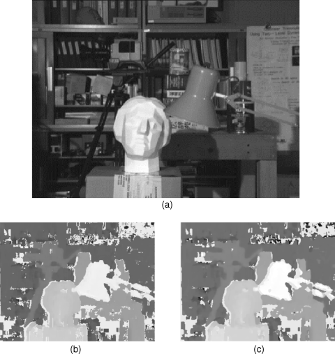
An obvious possibility for hole-filling is to apply a symmetric Gaussian filter. Equation 4.47 explains how that filter works around a given point x, y. If this point lies in a hole but in the vicinity of its edge, then the points given by the parameters μ and υ outside the hole contribute to the information at point x, y in the hole. That way, the hole is partly filled with information from neighboring pixels and the edge is smoothed. By choosing a large enough window for the filtering, the hole could even be filled completely. The image in Figure 4.44a obtained after warping exhibits white areas along the right edge and along the edge of the face and the table. These holes were filled by symmetric Gaussian smoothing as demonstrated in Figure 4.44b. However, closer inspection above the head of the man as shown in Figure 4.44c reveals that white artifacts and distortions have appeared. After asymmetrical smoothing with σx = 10 and σy = 90 these artifacts and vertical distortions disappear as demonstrated in Figure 4.44d. So asymmetric Gaussian filters are a powerful means for hole-filling.
Figure 4.44 (a) Image after warping exhibiting white stripes (holes). (b) Figure 4.44a after filling the holes by a symmetric Gaussian filter. (c) Enlarged head from Figure 4.44b showing a white stripe artifact. (d) Removal of artifact in Figure 4.44c by asymmetric filtering.
It was observed that filter interpolation, such as Gaussian filtering, results in artifacts in highly textured areas. Further, to fill large holes requires a large size of window for the filter. This, however, cannot preserve edge information as edges become blurred by smoothing. So a method to fill holes while keeping the PSNR and the image quality is needed. One way to achieve this consists of an edge-dependent depth filter, edge-oriented interpolation, and vertical edge rectification [35].
For the edge-dependent filter, in a first step the location of the edge has to be determined. This can be achieved, for example, by a search along a fixed direction in the image shown in Figure 4.11 and explained in the accompanying text. Once the edges are detected, the sharp increase in height is smoothed in the horizontal viewing direction. This increases for both eyes the visibility of the so far occluded area behind the edges, which decreases the size of the hole or even suppresses the occurrence of a hole. As a consequence this method enhances the quality and the PSNR of a warped image.
The functioning of edge-oriented interpolation is explained in Figure 4.45. This method detects the minimum difference in intensity in four orthogonal directions providing two minima. Then the center of the hole is filled with the mean intensity of the two minima. This works best for smaller holes which are adapted in a somewhat subdued way to the environment.
Figure 4.45 Edge-dependent filter for interpolation.
Vertical edge rectification detects vertical lines near an object boundary. If a depth along this line is inconsistent with the vertical, it is adjusted to a consistent depth. Figure 4.46a shows a figure before edge rectification, while Figure 4.46b depicts it after rectification.
Figure 4.46 Head (a) before and (b) after vertical edge rectification.
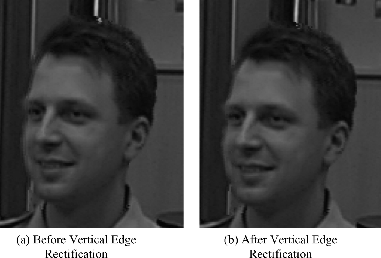
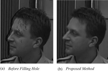
Figure 4.47a shows the same head before hole-filling with a disturbing edge along the left side of the head, while Figure 4.47b depicts it after application of the edge-oriented improvements. The lining at the edge has disappeared and no new artifacts and distortions have shown up. Measurements of the PSNR evidence that the edge-oriented method combined with smoothing enhances the PSNR by 6 dB.
Figure 4.47 Head (a) before hole-filling and (b) after edge-oriented hole-fillings.
4.7.4 Special Systems for Depth Image-Based Rendering (DIBR)
DIBR can be based on a multitude of different depth cues such as motion vector and motion parallax, intensity, contrast, chrominance, or geometrical perspective to name only a few. This entails the problem of how these many contributions can be fused into one pair of left and right images. A further topic is which selection entails the least computational load.
We shall now present some special DIBR systems, which differ in the selection of depth cues and in the fusion process. As a special feature for products which may become important in the near future, we can generate from all these cues a new 2D image with an enhanced depth perception compared to the original 2D version. This solution is called a depth-aware 2D video. The 3D video may have the format of a regular single view or of a multiview video.
The first system is based on three depth cues: depth from motion parallax (DMP), depth from geometrical perspective (DGP), and depth from relative position (DRP) [37, 38]. The block diagram in Figure 4.48 shows these selected cues and their processing to a depth-aware 2D display and to a single view and multiview 3D display. The properties of the three cues are investigated for blocks within the given image.
Figure 4.48 Block diagram for a DIBR system using three special depth cues.
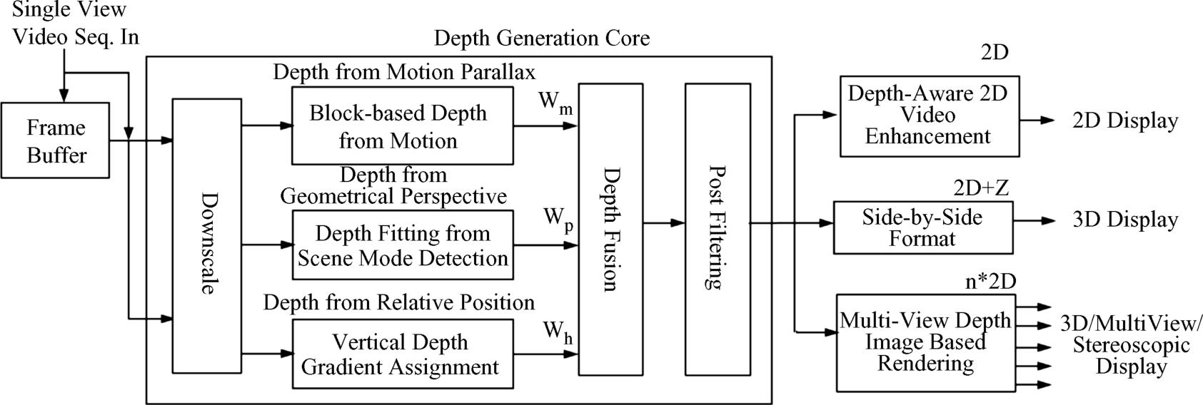
For the DMP the motion of a block vector MVblock was determined by minimizing the energy function [37]
(4.53)![]()
where for the displacement or the disparity d(x, y) in Equation 4.35b, the difference in the motion vectors of the block being investigated to its neighboring block is used. The SAD known from Equation 4.4 is complemented by the motion vectors as known from Equation 4.12 and Figure 4.11a and b. The minimization provides the displacement d(x, y) with the motion vectors MVx and MVy in the x- and y-directions as
(4.54)![]()
where λp is a scaling factor to relate the motion to depth.
The motion of the cameras has to be excluded from the determination of the disparity d(x, y), which is performed in Figure 4.48. To this end the concept using the baseline of the cameras in Figure 4.37 and the relationship between baseline and depth in Equations 4.1e,f are used. For various frames indicated by t, t + 1, t + 2,. . ., t + 4 in Figure 4.49 the pertinent baselines are determined. The baseline which provides the disparity closest to the estimated disparity DmaxO in Equation 4.52 is selected. As this selection is the closest match to DmaxO it is assumed that the motion of the camera is compensated best.
Figure 4.49 Baselines for various frames.
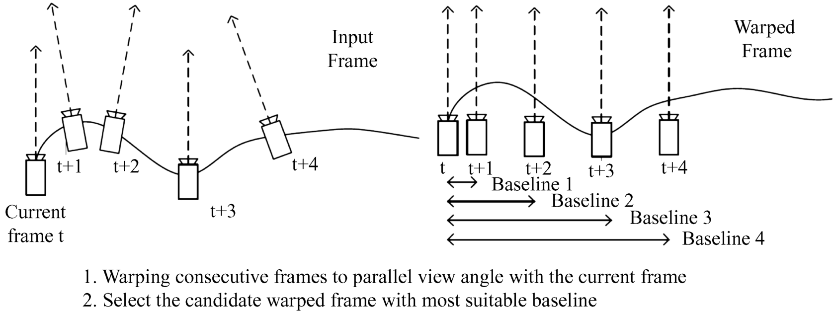
The DGP cue was based on scenes and their structural analysis. For this analysis the algorithm focusing on similarities like SSIM in Equation 4.22 can be used to provide a similarity index between scenes in a sequence of frames. For an interpretation of the result of the structural analysis, two structures with extrema in disparity, such as DmaxO known from Section 4.7.2 and the vanishing point with zero disparity, are introduced. The two blocks with disparities matching the disparities of the two structures are now a known number of pixels apart from each other. This can also be given by a disparity in cm, which represents a measure of how much the right and the left images have to be apart from each other. This distance has to be fitted by scaling factors in the range DmaxO to zero imposed by the display.
Finally the DRP detects the horizontal edge of video frames. These edges indicate the relative positions in the DRP. For finding these positions an edge detection algorithm based on edge-dependent Gaussian filters [36] is used. The distances of these positions, again in disparities, determine the difference between the left and the right eye images.
The depth or disparity data from DMP, DGP, and DRP have to be fused into one value for shifting the images from the intermediate or center image to the right and left eye images according to Equations 4.1e,f repeated here as
where the + sign applies for the location er of the right eye image and the −sign for el. This is the warping process shown in the block diagram in Figure 4.50[37]. The fusion of the depth cues can be done according to a priority measure favoring the largest disparity or by the mean of the three disparities.
Figure 4.50 Block diagram for individual steps in the DIBR process.
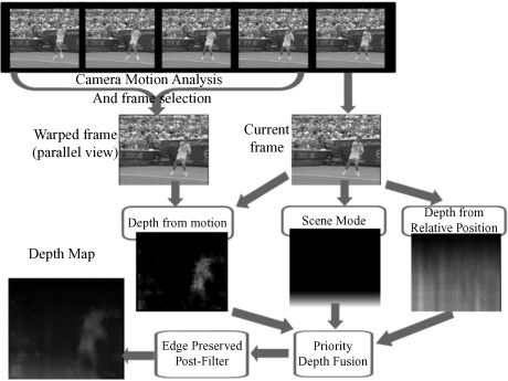
Finally in Figure 4.50 the fused images undergo a bilateral, most often Gaussian filtering to smooth out the block artifacts.
For the original 2D image of the tennis player in Figure 4.51a, test persons evaluated that a block size of 4 × 4 or 8 × 8 pixels yielded the best results. The depth-aware 2D video in Figure 4.51b conveys a moderately enhanced sensation of depth. Figure demonstrates the 3D multiple view represented by the left view in Figure 4.52a, the intermediate view in Figure 4.52b, and the right view in Figure 4.52c.
Figure 4.51 The original tennis player in (a) and (b) its depth-aware version.
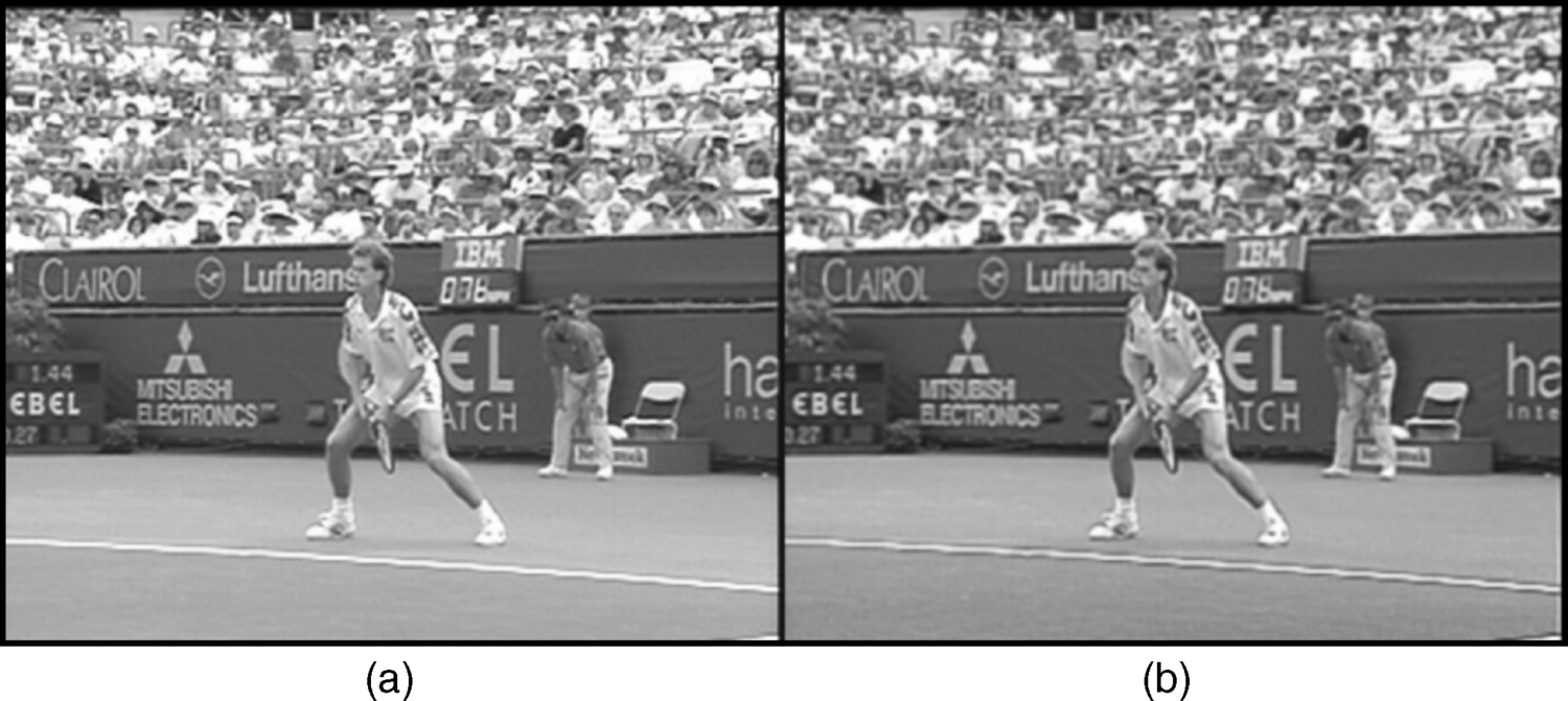
Figure 4.52 The multiview tennis player: (a) left eye view; (b) center view; and (c) right eye view.
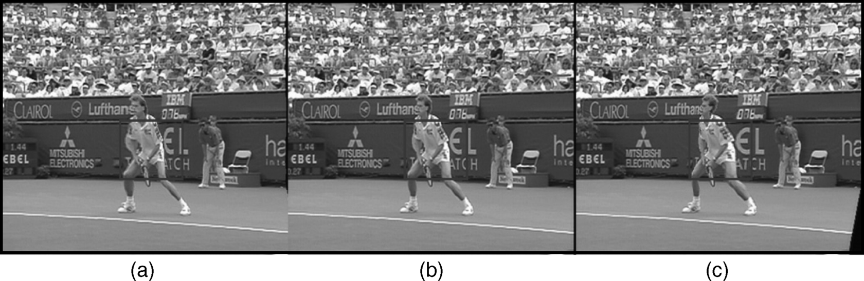
A very appealing and technologically more easily realizable approach to DIBR presented in [39, 40] is based on a selection of depth cues with a smaller computational complexity retrieved from a single image and very proficiently not from several frames. The objective is to enhance human depth perception rather than generate a physically correct depth map. The latter is, as a rule, associated with time-consuming processing steps, as we have encountered in Section 4.7.3. In view of this, algorithms based on motion parallax are excluded due to their computational load. This should lead to a faster and easier-to-implement algorithm. The depth cues selected are, according to Figure 4.53, depth gradients based on edge information. We have already encountered such types of gradients in Section 4.6.3 together with gray shade analysis and luminance setting. In Figure 4.27c we noticed that a luminance setting increasing in brightness from top to bottom, thus exhibiting a gradient, conveys a surprising sensation of depth [30]. This feature led to an advanced DIBR system in [40].
Figure 4.53 (a–e) Block diagrams of the five depth gradient approaches.
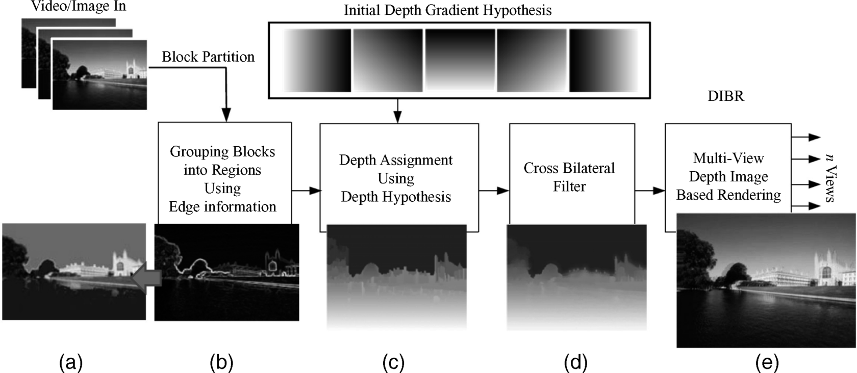
Images exhibit edges which, as a rule, announce a change in image content, such as texture, contrast, or depth. The edge detection algorithm investigates an image block-wise and not more cumbersomely pixel-wise, thus saving computation time. Blocks which share the same assumption of depth are grouped into regions as depicted in Figure. In the first step in Figure 4.54a the given original image is divided into, as an example, 4 × 4 blocks which in Figure 4.54b are linked and numbered. The links have a weight given by
(4.56)![]()
where the mean of color or luminance in linked blocks is used. If the difference diff(a, b) between the blocks is high, the two blocks possess a low similarity and the link is removed. In other words, in the case of removal there is an edge between the blocks separating the blocks. After removal of all such links with a high diff-value, the still linked regions of equal similarity in Figure 4.54c are obtained. To each still linked region R a hypothetical disparity(R) is assigned as
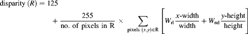
where 125 and 255 are depths in an 8-bit depth map; Wrl is the gradient of geometrical perspectives such as luminance or gray shade from a pixel x in the center of a block in the horizontal direction to the end of the block; and the same is true for Wnd which is the gradient in the vertical direction. The gradients can of course be positive or negative and are constrained by
(4.58)![]()
Figure 4.54 Creation of blocks with equal similarity: (a) the given image divided into 4 × 4 blocks; (b) linking and numbering of the blocks; (c) removal of high-weight links between blocks forming regions; (d) assigning gray shades to the regions due to the disparity(R) in Equation 4.57.
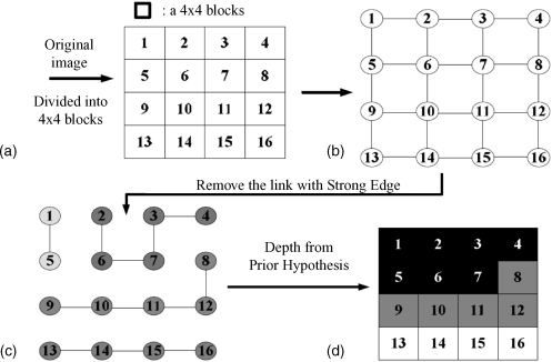
As a result disparity(R) indicates in which of the five directions in Figure 4.55a–e the luminance, contrast, or gray shade increases. This gradient is then associated with the region R. If this association fails, then the most often occurring gradient from the top down to the bottom is assigned as a default mode. The total disparity map consists of the combination of the disparity maps of all regions R with a gradient from Figure 4.55a–e assigned to them.
Figure 4.55 (a–e) The five depth map gradients (gradients of gray shades).

A large disparity(R) indicates blocks closer to the viewer. This coincides with the physiological fact that a large luminance, contrast, or gray shade appears to be closer to the viewer. An objectively correct determination of disparity or depth is not desired.
As artifacts between the blocks and regions may show up, a Gaussian filter for smoothing is applied. The filtered disparityf(x) is
(4.59)![]()
where n(xi) denotes the intensity in the pixel xi, Ω(xi) are the neighboring pixels to xi, and N(xi) represents the normalization factor. The window size depends on the block size. Figure 4.56a shows such a disparity map with depth-assigned blocks, while Figure 4.56b depicts its filtered version.
Figure 4.56 (a) Depth-assigned blocks, a disparity map, and (b) its bilaterally filtered version.
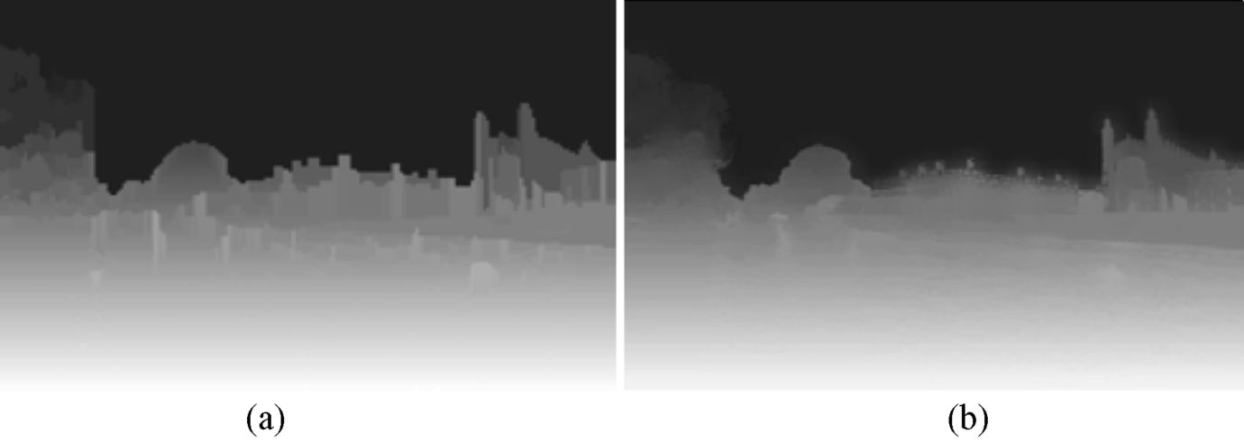
Finally the disparities due to Equations 4.1e, repeated in Equation 4.55, are used to generate the right and the left images.
If motion parallax is included, as a rule an improved depth quality can be achieved. However, the presented DIBR method without motion parallax is simple, fast, and effective.
As an example, Figure 4.57 shows on the left the original soccer scene, with the disparity map next to it obtained by the DIBR method in [40] presented above, aiming for a most objective disparity map. The third image in Figure 4.57 is the disparity map provided by the method in [40], based on hypothetical disparities. The difference in disparities is striking. In the hypothetical map the gradient of disparity is visible, which is not the case in the other map.
Figure 4.57 The soccer pitch (a) the original image; (b) the disparity map; and (c) the disparity map obtained by the disparity(R) in Equation 4.57.
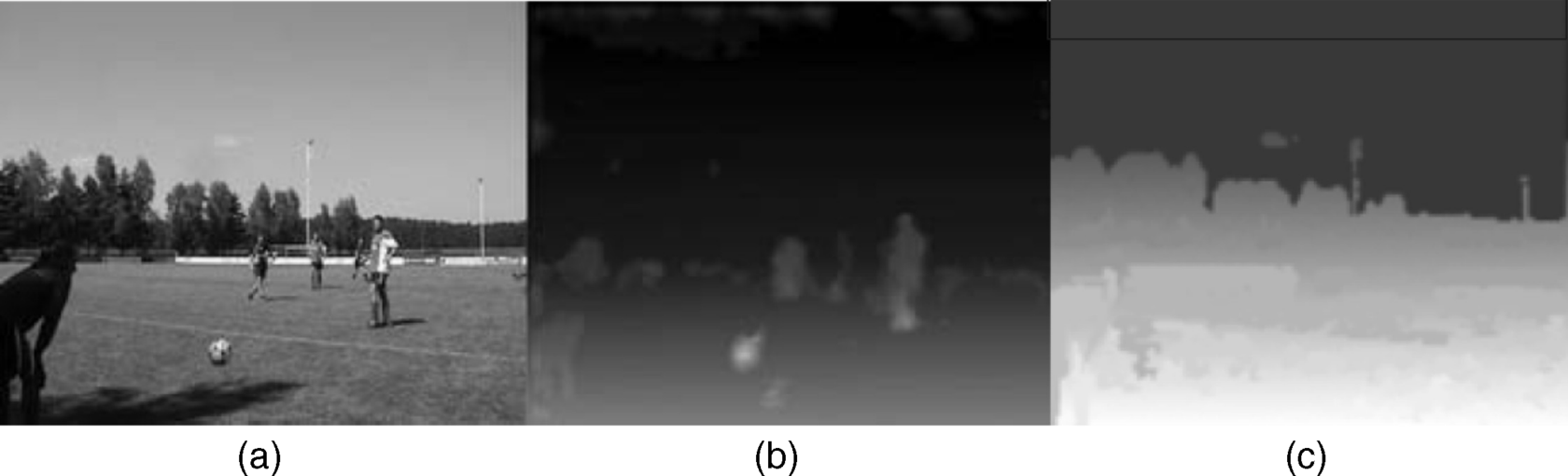
In conclusion of this discussion on quality, attention is drawn to the need for establishing a metric characterization of the quality of 3D images. The SSIM algorithm in Section 4.4, dealing with structural similarities derived from luminance, contrast, and a cross-correlation of the two, offers a generally accepted index of subjective satisfaction with image quality. However, this index does not include the sensation of depth.
The approach for the inclusion of depth in a quality metric in [41] is briefly outlined. It starts with an approximation of disparity valid for distances of an object that are not too large. The disparity map associates pixels with the same disparity in the left and the right views with the same point in the object space. So a relationship between the pixels in the two views and depth is established. The task is to combine this relationship into one single cyclopean image and characterize it with the SSIM algorithm. The necessary steps are shown in Figure 4.58. The cyclopean image is created by assigning to a given depth the pixels from the left and the right views. Allocated to this location in a depth map is an intensity corresponding to both views [42]. If the right and left eye views are undegraded, this cyclopean image serves as a reference image. A degraded image occurs, for example, when the image is blurred by a convolution or after JPEG compression has been applied. The difference between the undegraded and the degraded image is determined by the SSIM algorithm according to Equation 4.22 for each point x, y in the two cyclopean images. This provides an SSIM map describing the similarity between the two images which is considered to be a metric for the quality of the degraded image 3D videos. The authors of [42] call this a preliminary study on a metric for 3D images. They point out a difficulty which arises if, for example, a point in the left view cannot be matched to a point in the right view. In this case zero disparity is assigned, which means that no depth information is available. This case occurs if an object is occluded for one of the two views. Then the point in question does not meet the consistency test [13] in Section 4.3.1. If this occurs in a large area the quality test for depth is uncertain. One way out could be to include different viewpoints of the object as treated in the VSSIM algorithm [4] found in Section 4.4. Further, one could apply the hole-filling methods treated in Section 4.7.3. This could help because occlusions may disappear or are rendered smaller from different viewpoints. However, this requires more detailed investigations.
Figure 4.58 The procedure for a 3D quality test including depth.
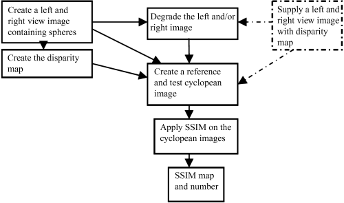
The author gratefully acknowledges permission to reproduce figures and tables granted by the institutions named below. The sources of the figures and tables are also listed below together with their corresponding numbers in this book.
Institute of Electrical and Electronics Engineers (IEEE)
IEEE Transactions on Image Processing, vol. 13, no. 4, 2004
p. 601, figures 1, 2a–f; p. 607, figures 5a–d; p. 608, figures 6a–l,
p. 610, figures 8a,d; p. 1338 (2003), figure 2
Reproduced as Figures 4.2, 4.13a–f,4.14a℃d, 4.15a–l, 4.16a,b, 4.17
IEEE Transactions on Pattern Analysis and Machine Intelligence, vol. 22, no. 7, July 2000, p. 680, figure 5a
Reproduced as Figure 4.7a
Proceedings of the IEEE Workshop on Stereo and Multi-Baseline Vision (SMBV'01), figure 2
Reproduced as Figures
IEEE Transactions on Acoustics, Speech, and Signal Processing, vol. ASSP-31, no. 5, October 1983, figure 1
Reproduced as Figure 4.30
IEEE Transactions on Broadcasting
vol. 51, no. 2, June 2005, p. 195, figures 2, 3, 5a, 5c, 7a, 7c, 8
Reproduced as Figures 4.34a,b, 4.35a,b, 4.36a–c
vol. 54, no. 2, June 2008, figures 8, 9b,c, 7e, 5a, 12a,d, 13a,d, 15a–c, table p. 193
Reproduced as Figures 4.38a,b4.40a,b, 4.41a,b, 4.42a,b, 4.43a–c, Table 4.1
IEEE International Conference on Multimedia and Expo (ICME), 2005
figures 1, 3, 4, 5, 6a,d
Reproduced as Figures 4.33, 4.45, 4.46a,b, 4.47a,b
IEEE International Conference on Consumer Electronics, 2009
p. 2 figures 2, 5, and vol. 56, no. 3, August 2010, p. 1740, figures 2, all lines of 5, 11
Reproduced as Figures 4.49, 4.50, 4.53a–e, 4.54a–d, 4.55a–e, 4.57
Society for Information Display (SID)
SID – Symposia and Conferences
| SID 07 p. 1161, figures 1c–e, 2, 3 | reproduced as Figures 4.12a, b, 4.10, 4.11 |
| SID 95 p. 859, figures 2, 6, 10 | reproduced as Figures 4.21, 4.22, 4.23 |
| SID 98 p. 686, figures 1, 2, 3 | reproduced as Figures 4.24, 4.25a, b |
| IDW 09 p. 2033, figures 4, 5c,e | reproduced as Figures 4.28, 4.29a, b |
| IDW 09 p. 2034, figures 3, 1, 6, 7 | reproduced as Figures 4.26, 4.27, 4.31, 4.32 |
| SID 09 p. 123, figures 1, 5, 6 | reproduced as Figures 4.48, 4.51a, b, 4.52a, b, c |
| SID 10 p. 522, figure 2 | reproduced as Figure 4.58 |
1. Eskicioglu, A.M. and Fischer, P.S. (1995) Image quality measures and their performance. IEEE Trans. Commun., 43, 2990.
2. Wang, Z. et al. (2003) Objective video quality assessment, in Handbook of Video Databases: Design and Applications (eds. B. Fuhrt and O. Marques), CRC Press, Boca Raton, FL, p. 1041.
3. Wang, Z. et al. (2004) Image quality assessment: from error visibility to structural similarity. IEEE Trans. Image Process., 13, 600.
4. Wang, Z. et al. (2003) Multiscale structural similarity for image quality assessment. IEEE Trans. Image Process., 12, 1398.
5. Okutomi, M. and Kanade, T. (1992) A multiple base-line stereo. IEEE Trans. Pattern Anal. Mach. Intell., 15, 353.
6. Watson, A.B. (1993) The cortex transform: rapid computation of simulated neural images. Comput. Vision, Graphics, Image Process., 39, 311.
7. Simonelli, E.P. et al. (1992) Shiftable multi-scale transforms. IEEE Trans. Inf. Theory, 38, 587.
8. Watson, A.B. and Solomon, A. (1997) Model of visual contrast gain control and pattern masking. J. Opt. Soc. Am., 1419, 2379.
9. Yu, W. and Hanske, G. (1994) Picture quality evaluation based on error segmentation. Proc. SPIE, 2308, 1454.
10. Lin, J. and Moulin, P. (2001) Information-theoretic analysis of interscale and intrascale dependencies between image wavelet coefficients. IEEE Trans. Image Process., 10, 1647.
11. Hamah, M.J. (1989) A system for digital stereo matching. Photogram. Eng. Remote Sensing, 55 (12), 1765.
12. Muehlmann, K. et al. (2001) Calculating dense disparity maps from color stereo images, an efficient implementation. Proceedings of the IEEE Workshop on Stereo and Multi-Baseline Vision.
13. Fua, P. (1993) A parallel stereo algorithm that produces dense depth images and preserves image features. Mach. Vision Applic., 6, 35.
14. Sun, C. (1997) A Fast Stereo Matching Method, Digital Image Computing: Technique and Applications, Massey University, Auckland, New Zealand, p. 95.
15. Scharstein, D. et al. (2001) A taxonomy and evaluation of dense two-frame stereo correspondence algorithms. Proceedings of the IEEE Workshop on Stereo and Multi-Baseline Vision.
16. Scharstein, D. and Szeliski, R. (2001) A taxonomy and evaluation of dense two-frame stereo correspondence algorithms. Microsoft Research, MSR-TR-20001-81, Nov. 2001 (extended version of [15]).
17. Ku, J.S. et al. (2007) Dense disparity map calculation from color stereo images using edge information. SID 07, p. 1160.
18. Wang, Z. (2001) Rate scalable foveated image and video communications, PhD thesis, University of Texas at Austin.
19. Wang, Z. and Borik, A.C. (2002) A universal image quality index. IEEE Signal Process. Lett., 9, 81.
20. Wendell, B.A. (1995)Foundation of Vision, Sinauer Associates, Sunderland, MA.
21. Zitnick, C.L. and Kanade, T. (2000) A cooperative algorithm for stereo matching and occlusion detection. IEEE Trans. Pattern Anal. Mach. Intell., 22 (7), 675.
22. Lucas, B.D. and Kanade, T. (1981) An iterative image registration technique with an application to stereo vision. International Joint Conference on Artificial Intelligence, p. 674.
23. Tomasi, C. and Kanade, T. (1991) Detection and tracking of point features, Carnegie Mellon University Technical Report CMU-CS-91-132.
24. Shi, J. and Tomasi, T. (1994) Good features to track. IEEE Conference on Computer Vision and Pattern Recognition, p. 593.
25. Lucas, B.D. and Kanade, T., An iterative image registration technique with an application to stereo vision, and Horn, B.K.P. and Schenk, B.G., Determining optical flow, Carnegie Mellon University ECE CVRR CSE p. 291, 11-1-01.
26. Adelson, S.J. et al. (1991) Comparison of 3D displays and depth enhancement techniques. SID 91, p. 25.
27. Murata, M. et al. (1995) Conversion of two-dimensional images to three dimensions. SID 95, p. 859.
28. Murata, M. et al. (1998) A real time 2D to 3D image conversion technique using computed image depth. SID 98, p. 919--922.
29. Iinuma et al. (2000) Natural stereo depth creation methodology for a real-time 2D to 3D image conversion. SID 2000, p. 1212.
30. Kao, M.-C.A. and Shen, T.-C. (2009) A novel real time 2D to 3D conversion technique using depth based rendering. IDW'09, p. 203.
31. Oflazer, K. (1983) Design and implementation of a single-chip 1D median filter. IEEE Trans. Acoust., Speed, Signal Process., ASSP31 (5).
32. Zhang, L. et al. (2004) Stereoscopic image generation based on depth images. IEEE International Conference on Image Processing, p. 2993.
33. Zhang, L. and Tom, W.J. (2005) Stereoscopic image generation based on depth images for 3D TV. IEEE Trans. Broadcast., 51 (2), 191.
34. Kim, D. et al. (2008) A stereoscopic video generation method using stereoscopic display characterization and motion analysis. IEEE Trans. Broadcast., 54 (2), 188.
35. Chen, W.-Y. et al. (2005) Efficient depth image based rendering with edge dependent depth filter and interpolation. IEEE International Conference on Multimedia and Expo (ICME), p. 1314.
36. Akutsu, A. et al. (1992) Video indexing using motion vectors. Proc. SPIE VCIP, 1818, 1522.
37. Cheng, C.-C. et al. (2009) A quality scalable depth-aware video processing system. SID 09, p. 123.
38. Cheng, C.-C. et al. (2009) A block based 2D to 3D conversion system with bilateral filter. IEEE International Conference on Consumer Electronics.
39. Cheng, C.-C. et al. (2010) An ultra low cost 2D to 3D video-conversion system. SID 10, p. 766.
40. Cheng, C.-C. et al. (2010) A novel 2D to 3D conversion system using edge information. IEEE Trans. Consum. Electron., 56 (3), p. 1739--1745.
41. D'Dosterlink, W. et al. (2010) New methodology for evaluating quality of stereoscopic images. SID 10, p. 522.
42. Howard, I. and Rogers, B. (1995)Binocular Vision and Stereopsis, Oxford University Press, New York.