Chapter 12

Coding Methods for Depth Videos

12.1. Introduction

Recent advances in the domain of three-dimensional (3D) cinema and the emergence of new multimedia services such as free viewpoint television (FTV) or 3D television (3DTV) have created a need for new, lighter and less costly 3D video formats. This is a current research focus in both the academic and industrial domains.

The first proposal for 3D video representation was the classic stereoscopic format (stereoscopic 3D (S3D)). This consists of two views of the same scene, recorded by two cameras separated by a certain distance (the baseline). The association of a different view with each of the spectator’s eyes produces a 3D effect by stereoscopy.

Mixed resolution stereo (MRS), followed S3D. This format exploits the theory of binocular suppression, which stipulates that if the two views have a different image quality, the perceived quality of the stereoscopic video will be closer to that of the view with the highest quality [BRU 09]. In practice, this means that if one of the two views is encoded at a lower resolution, the overall quality perceived by the spectator will remain good. Therefore, MRS allows us to reduce the cost (in terms of bit rate) of encoding and transmitting 3D information.

However, two views are not sufficient to deliver wide-range fluid 3D content. This fluidity is necessary for applications such as FTV, where the user has the ability to navigate between different 3D scenes using a controller. Furthermore, for 3DTV, two views are not sufficient to ensure that a spectator not situated directly in front of the screen will experience 3D. The multi-view video (MVV) format was introduced to respond to these issues. The approach involves N views representing the same scene, captured by N cameras arranged and spaced in a specific manner. However, this format is generally costly due to the bit rate required to code and transmit N views.

Depth-based formats are the most recently proposed type of 3D video formats. They are still the subject of study and research, both in the academic sphere and in industry. First, the video + depth (V+D) format consists of a texture view and an associated depth view. Using these two views, a second texture view can be extrapolated at a different position in space, using a technique known as depth image based rendering (DIBR). The newly created texture view and the original view allow stereoscopic viewing of the 3D video. If more views are required, the multiview video + depth (MVD) format may be used. This involves N texture views and their associated depth views. Several intermediate views may then be interpolated using the DIBR technique.

The main advantage of depth-based formats is their low cost, as the bit rate required to code and transmit depth information is lower than that needed for texture information. However, the acquisition of depth videos is not simple. The algorithms for depth estimation, such as stereo matching, are not perfect; the estimated depth often presents artifacts. Obtaining depth directly using time-of-flight cameras is an interesting alternative, but the technology has not yet reached a sufficient level of maturity. Another possibility would involve estimating depth, then cleaning each depth map manually, but this is only an option for major cinema studios with the necessary financial resources. Nevertheless, depth-based formats present considerable potential and are currently the object of standardization efforts, allowing these formats to gradually take their place in industry.

The delivery of 3D content is costly in terms of bit rate. High compression gains are required in order to stay within the bandwidth authorized by service providers. In cases where depth-based formats are used, depth videos must be compressed (as in the case of texture videos). However, depth videos have different characteristics from classic texture videos, and, therefore, specific depth compression algorithms must be used. In this chapter, we will present the different methods or tools that have been developed to code depth videos.

This chapter is organized as follows: section 12.2 presents an analysis of depth maps and their specific characteristics. It also includes a discussion of different types of redundancies, which may be exploited in order to maximize compression levels of depth videos. Three main categories of depth coding tools can thus be defined. These tools are presented in section 12.3, with examples. Finally, section 12.4 concludes the chapter.

12.2. Analyzing the characteristics of a depth map

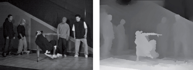
A depth map associates a depth value (a distance to the camera) with each pixel in the texture picture. It is therefore a single-component image (Luma), essentially made up of smooth regions separated by contours, as shown in Figure 12.1. The depth map is not affected by illumination and contains neither textures nor shadows. Depth compression may be carried out in three different ways. First, the intrinsic characteristics of depth maps may be exploited, either at the block level in the coding loop, or in higher level data structures, such as slices or frames. Second, correlations with the associated texture may be exploited. Texture and depth are highly correlated, notably in the contours of objects. Specific depth transforms or certain coding decisions may also depend on texture information. Finally, as depth videos are not shown on screen but rather used to synthesize intermediate views, depth coding may be optimized for the quality of these synthesized views. This means that new distortion models, considering the effects of depth coding on synthesized views, may be established.

As a result, we may identify three broad categories of depth coding methods: methods using the intrinsic characteristics of depth maps, those using correlations with associated textures and, finally, those which optimize depth coding for the quality of synthesized views. The following section provides a detailed overview of each category, giving examples of tools proposed either in the literature on the subject or in response to the Moving Pictures Expert Group (MPEG) Call for Proposals (CfP) for 3D video in November 2011 [IEC 11].

12.3. Depth coding methods

In this section, we present the three categories of methods used in depth coding, with examples of tools used in each category.

12.3.1. Methods using the intrinsic characteristics of depth maps

These methods may be grouped into two subcategories: tools that operate at the block level and those that operate at a higher level. The first subcategory uses the block coding structure found in classic video encoding, with specific modifications through the introduction of new coding modes, better suited for depth coding. The second subcategory considers depth images as a whole (without the use of blocks).

12.3.1.1. High-level coding tools

The first example of a coding tool in this category is the reduction in resolution of depth maps before coding, which may be considered as a depth data compression technique [RUS 11]. The artifacts associated with up-sampling the depth map after decoding are minimal, and we may thus obtain considerable compression gains by simply reducing the resolution of the depth videos to be encoded. The test model for advanced video coding (AVC) based 3DV solutions [HAN 12], defined in March 2012, proposes down-sampling depth videos to a quarter of their initial resolution (half in each direction) before encoding.

Another tool involves reducing the resolution of motion vectors used in depth coding. The eight-tap filters used for motion-compensated interpolations, as defined in the sixth High Efficiency Video Coding (HEVC) working draft [BRO 11], produce artifacts on sharp edges in depth. As a result, motion (or disparity) compensated predictions may be modified to avoid interpolations, meaning that only full-pel motion vectors and disparity vectors will be used. The reduction in the precision of motion vectors also reduces the bit rate required to transmit the motion vector differences [SCH 11].

View synthesis prediction is another efficient coding tool, used for both texture and depth [RUS 11]. Using a reconstructed depth map at view 0, a depth map may be synthesized for view 1 and used as a predictor to code . Synthesizing an image involves making the pixels of a source image correspond to a destination image , situated at a required position (view), as follows:

[12.1]

where f is the focal distance, B is the distance between cameras (for views 0 and 1 in our case), D(x, y) is the value of the disparity at position (x, y) and d(x, y) is the depth value at position (x, y). As, in this case, we are synthesizing a depth map, and we obtain s(x, y) = d(x, y).

Another useful tool is the compensation [DOM 11] for weighted prediction. Different frames of the same view or different views at the same instant in time, for a depth video sequence, may have different extremal depth values (denoted as and ). As depth maps are rescaled in the interval [0, 255], different depth images may be scaled differently. In this case, the use of a depth map as the reference image for another depth map would lead to poor predictions and inefficient compression. To solve this problem, coherent scaling needs to be applied for all depth maps in question. This is easy to achieve using extremal values. For example, if a depth map with extremal values and is used as the reference image for a current depth map with extremal values and , the scaling for the current depth map is carried out as follows:

[12.2]

where is the original depth value and is the rescaled value.

12.3.1.2. Block-based coding tools

The first tool for consideration in this category is the approximation of depth blocks using modeling functions, presented in [MER 08]. As the depth map is essentially made up of smooth regions separated by contours, a depth block may be approximated by four different types of functions: a constant function, a linear function, a constant piecewise function or a linear piecewise function. If no approximation can be found for the current block, then the block is divided into four blocks in a quad-tree manner. The process is repeated for each block until an approximation function is found for each leaf of the quadtree.

The same principle was used and improved in a contribution to the MPEG CfP for 3D video [SCH 11]. This contribution proposes four new Intra modes, two of which (mode 3 and mode 4) use texture information and will be discussed further in section 12.3.2.2. These modes are known as depth modeling modes (DMM). In mode 1, the current depth block is approximated by two constant regions, denoted by and , separated by a line segment DF, as shown in Figure 12.2. The predictor signal (or block) is thus made up of two regions, and the value P_i, where i = {1:2}, of each pixel in a region R_i is equal to the mean value of the pixels in the original block covered by R_i. Thus, P₁ and P₂ are transmitted to the decoder, along with the partition information, which consists of the beginning and end points (D and F) of the segment DF separating the two regions. In mode 2, P₁ and P₂ are transmitted without the partitioning information, which, in this case, is deduced from the neighboring blocks. However, the resulting partition may not be adequate for the current block. Thus, an offset F_off, correcting the arrival point of the straight line, as shown in Figure 12.2, is also transmitted in the bitstream.

While the first two tools involve Intra prediction, the adaptive 2D block matching (2D-BM)/3D block matching (3D-BM) selection tool concerns inter-prediction [KAM 10]. 2D-BM is the classic way in which an encoder, during a motion estimation stage, finds the temporal reference block that best corresponds to the current block. The correspondence is measured by the sum of squared errors (SSE), defined as follows:

[12.3]

where f is the original current block of size to code, and g is the temporal reference block, also of size . In this case, the search is carried out in two dimensions: horizontal and vertical. However, in depth videos, we also have motion in the depth direction. Search precision may thus be increased by extension to a third dimension. This idea is implemented in 3D-BM. Thus, the best temporal correspondence is the one that minimizes the new formulation of the SSE, as follows:

[12.4]

3D-BM is more efficient than 2D-BM for high bit rates, where the gains produced by the reduction of distortion are higher than the costs associated with the addition of a new component for motion vectors. Inversely, at low bit rates, 2D-BM is more efficient than 3D-BM. Adaptive 2D-BM/3D-BM selection evaluates the R-D cost for the coding of each block with 2D-BM and 3D-BM and chooses the method that minimizes cost. The choice is then sent in the bitstream for decodability. This adaptive selection is more efficient than pure 2D-BM and 3D-BM for middle bit rates.

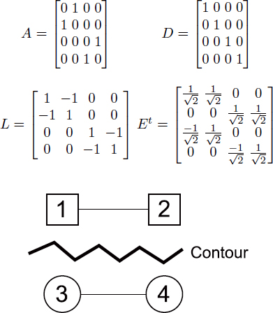
Transforms may also be adapted for depth content. Edge-adaptive transforms (EAT) are proposed in [SHE 10]. These transforms directly take into account the contours of a depth block, and consequently enable a reduction in the number of non-zero coefficients after filtering. An initial contour detection stage is carried out on the residual block, and a binary contour map is established. An adjacency matrix A is then calculated based on this binary contour map, as follows:

[12.5]

Using the adjacency matrix, a degree matrix D may be calculated as follows:

[12.6]

The Laplacian matrix L may thus be calculated as the difference between D and . Finally, from L, the transform matrix E^t may be calculated using the cyclical Jacobi method. Take a simple example of a residual of size , as shown in Figure 12.3. In this example, matrices A, D, L and E^t will be equal to:

We can prove that for a residual of size , piecewise constant with M constant regions, the EAT coefficients will be composed of at most M non-zero coefficients and zero coefficients. As a result, coding efficiency may be improved by using EAT instead of the classic discrete cosine transform (DCT). However, the use of EATs requires transmission of the binary contour map, which will not otherwise be available to the decoder. Thus, EATs may be less effective than the DCT. An R-D criterion may be specified in order to identify the best transform, but this choice must also be transmitted to the decoder.

12.3.2. Methods exploiting correlation with associated textures

There is a strong correlation between the texture and depth components, and this correlation can be exploited to produce coding gains at depth level. First, the prediction modes used for different depth blocks may be selected according to the information present in texture. Second, the prediction information for depth blocks, such as motion vectors, reference picture indices or Intra modes, may be inherited from texture blocks. Finally, texture information may be used to construct spatial transforms better suited to depth coding in order to increase coding efficiency.

12.3.2.1. Inheritance/selection of prediction modes

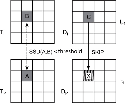
Depth block skip (DBS), is a tool presented in a contribution [LEE 11b] to the MPEG CfP for 3DV. It allows coding of a depth macroblock in Skip if the temporal correlation in texture is judged to be sufficient. If there is a high temporal correlation in texture, there is a high chance that this correlation will also be strong with depth, and, in this case, the best mode (in terms of R-D) for a depth block will be Skip. In DBS, this block is forced to be coded using Skip, meaning that the Skip mode does not need to be signaled. Formally, for a current depth block X to be coded in the depth frame D_i at instant i, we calculate the sum of squared differences (SSD) between A, the colocated block in the reconstructed texture frame T_i, and B, the colocated block in the reconstructed texture frame T_i–1. If this SSD is below a certain threshold, we consider that the temporal correlation in texture – and also in depth – is high, and we code X in Skip mode with C, the colocated block in D_i–1, as a candidate, meaning that the prediction information for C will be inherited by X, as shown in Figure 12.4. This tool has certain drawbacks. First, it uses two texture frames to code a depth block. This represents a relatively large amount of additional information to use, only justifiable if the method produces significant gains in terms of depth compression, which is not the case. Moreover, using this tool, depth coding is subject to errors in the texture, which affect an access unit different to that of the current depth frame, thus reducing the robustness of the coding. Finally, the tool violates a general codec design principle, which stipulates that the parsing of the bitstream should be independent of signal processing applied to already decoded pictures.

In a more direct manner, Skip mode in depth may also be forced each time that the colocated texture block is coded using Skip [KIM 09]. The main idea behind this tool is that the spatial uniformity of movement in texture is likely to also be present in depth. Skip mode may not necessarily be chosen under normal circumstances due to the presence of certain artifacts inherent in the original depth, which create false movements. Imposing Skip mode on a depth block if it is chosen for the colocated texture block eliminates these artifacts, thus increasing the quality of views that will be synthesized with the current depth frame. The tool also produces compression gains due to the fact that no signaling is required for Skip mode. Finally, the tool also reduces the complexity of the encoder as it reduces the number of complex motion estimations and compensations to perform.

12.3.2.2. Inheritance of prediction information

Motion information (motion vectors + reference picture indices) is highly correlated between texture and depth, notably around object contours. In [SEO 10], a new mode, known as motion sharing (MS), is added to the list of existing modes (Intra, Inter, Skip). In this new mode, the motion information for a depth block is directly inherited from the corresponding texture block. No motion estimation is carried out. MS mode is not systematically imposed for depth blocks: an R-D criterion verifies the cost and compares it to those entailed by other prediction modes. MS is then selected only if it offers the lowest cost.

Motion parameter inheritance (MPI), introduced in [SCH 11], is another tool that allows inheritance of motion information from texture for depth, but the technique used is somewhat different. In MPI, there is no new prediction mode; the texture motion information and its partitions are considered as a new candidate for Merge mode for the current depth block. Merge is a coding mode, introduced in HEVC, in which the current block inherits prediction information from a given candidate, selected from a group of candidates (we thus speak of “competition” between different candidates). The selection is based on an R-D criterion, and only the index of the selected candidate is transmitted to the decoder in order to construct the predictor signal.

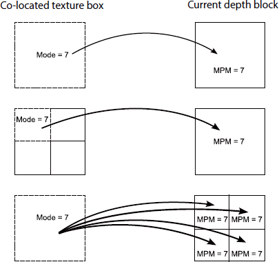
The Intra mode of a texture may also be inherited, as proposed in [BAN 11], for the colocated depth block. As we see in Figure 12.5, if the texture block is partitioned more finely than the depth block, the Intra mode of the top left block will be inherited. If, on the other hand, the depth block is more finely partitioned than the texture block, the Intra mode of the texture block will be inherited for all depth partitions. Here, inheriting the texture of the Intra mode means that the mode will be added to the list of most probable Intra candidates most probable mode (MPM) for the current depth block, where it will act as a predictor for the depth Intra mode.

The method described above involved inheritance of the texture Intra mode for all depth blocks. However, the Intra modes of the two components do not always match. In cases where there is no matching, inheritance of the texture Intra mode can lead to coding losses, as the inherited mode may replace a good spatial predictor in the list of MPM candidates. In [MOR 12], a study shows that texture and depth Intra modes are particularly correlated in areas where contours are clearly defined in texture. Thus, inheritance is only applied if a criterion measuring the sharpness of the contours present in the colocated texture block is above a certain threshold.

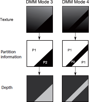
Texture information may also be used to define new Intra modes for modeling depth blocks. We have already discussed modes 1 and 2 in section 12.3.1.2. Mode 3 still seeks to approximate the depth block using two constant regions separated by a straight line, but in this case, the partition information is inherited directly from the texture. A simple thresholding of Luma texture samples may be used to separate the texture block into two distinct regions. This partition is used directly for the depth block. Thus, no partition information is transmitted as the same procedure may be carried out by the decoder. Constants and , on the other hand, must always be transmitted. Mode 4 operates in the same way as mode 3, except the depth block is divided into three constant regions, as shown in Figure 12.6 (this is known as “Contour” type partitioning, as opposed to “Wedgelet” partitioning, where the block is divided into two constant regions, as in modes 1, 2 and 3).

12.3.2.3. Spatial transforms

Texture information may also be used to construct spatial transforms suited to depth coding. Daribo et al. [DAR 08] propose an adaptive wavelet lifting scheme, in which short filters are applied to depth areas containing contours and long filters are applied to homogeneous depth areas. Contour detection is carried out in texture for decodability, and is based on observed correlations between texture and depth contours.

12.3.3. Methods optimizing depth coding for the quality of synthesized views

As depth maps are not shown on screen but rather used to synthesize views, the R-D model used in depth coding must consider distortion directly on synthesized views in order to optimize coding for the truly important aspects, i.e. the intermediate synthesized views. There are different methods, some of which effectively synthesize views (or parts of views) during depth coding, while others estimate this correlation using texture information. We will compare these different techniques in this section.

12.3.3.1. View synthesis optimization

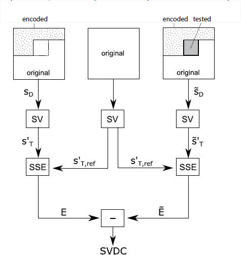
This method, known as view synthesis optimization (VSO), was proposed in [SCH 11]. It calculates the change in the distortion of the synthesized views caused by a change at the level of the current depth block. This metric, called synthesized view distortion change (SVDC), is calculated by synthesizing, in-loop, part of the view, which will be affected by a change in the depth block. Figure 12.7 shows how this metric is calculated. We consider a frame , where the depth block is in its original form. All succeeding blocks (in coding order) are in their original forms and all previous blocks have already been coded and reconstructed. Another depth frame is formed in the same way as , except the depth block is replaced by a reconstructed version as a function of the test (mode) being carried out. and are used to synthesize two texture views, and . Another view may also be synthesized using the original depth and texture frames. The calculation of the SSE between and gives E, and between and gives . The SVDC metric is simply equal to the difference .

This method is useful for three main reasons. First, it offers an exact measure of distortion, taking account of occlusions and disocclusions in the synthesized views. Second, the measure is related to a block. Third, using this metric, partial distortions are additive. If a block is divided into four sub-blocks, as is often the case when using quad-tree coders such as HEVC, the sum of the distortions caused by a change in each sub-block must be equal to the distortion caused by the corresponding change at the level of the whole block. SVDC guarantees this, as only the change in distortion in the synthesized view caused by a change in the current depth block is considered, and not the total distortion itself in the synthesized view. The main drawback of this method is the increase in complexity in terms of coding, as the metric is calculated (and thus a partial view synthesis is produced) for each possible depth partition. This view synthesis, although partial, requires a considerable number of operations, which may lead to a rapid increase in complexity.

12.3.3.2. Distortion models

Other distortion models do not effectively synthesize views in the depth coding loop; the synthesized view distortion is simply estimated. In [LEE 11a], the view synthesis distortion (VSD) metric is calculated as a distortion in the depth block, weighted by one-pixel texture translation differences:

[12.7]

where , and are, respectively, the original depth value, the reconstructed depth value and the reconstructed texture value at position (x, y). The value of α is defined as follows:

[12.8]

where f is the focal distance, B is the distance between the camera for the current view and the one for the synthesized view and are the extremal depth values.

In equation [12.7], we suppose that two adjacent pixels will remain adjacent after the warping operation, which is not always the case as occlusions or disocclusions may occur in synthesized views. To rectify this, and in equation [12.7] may be replaced by and , respectively, with and defined as follows:

[12.9]

Equation [12.7] is then corrected to take into account the regions of occlusion and disocclusion as follows:

[12.10]

where , the weight in texture, is defined as follows:

[12.11]

An even simpler distortion model, which estimates the distortion in synthesized views, was proposed in [KIM 09]. In fact, a distortion in a depth value at position produces a translation error in the synthesized view. A linear relationship exists between the two quantities, defined by:

[12.12]

where is defined by equation [12.8]. Moreover, there is a linear relationship between a global pixel translation t_x and the distortion measured in terms of the SSD of the original video signal translated by t_x. This relationship is defined by:

[12.13]

where V_(x,y) is the value of the original video signal at position (x, y). If several values of t_x are used and we calculate the corresponding distortions, we may define a scale factor s in the following way:

[12.14]

where and t_x are the vectors formed by the aggregation of multiple values of and t_x, respectively, and T is the transpose operator. For a certain position error , this parameter s provides an estimation of the resulting distortion in the synthesized view. If the views are synthesized from a left view and a right view, each contribution generally has a weight, for the left and (1 – p) for the right where :

[12.15]

A scale factor representing the global characteristics of may be defined by:

[12.16]

Using the two parameters above, a new distortion metric may be calculated in the following manner:

[12.17]

Finally, the Lagrangian cost function used in R-D optimization may be written as:

The main advantage of these distortion models, based on the disparity, is that they are less complex than solutions that effectively synthesize views (or parts of views) in the depth coding loop itself. However, the distortion evaluated in the second case is more precise than that obtained in the first case, a fact that may influence R-D decisions and increase coding efficiency.

Other depth coding tools aim to increase the sparsity of depth in the transform domain in order to increase coding efficiency. This is carried out by modifying the original values of the depth map before coding, as long as the change only affects synthesized views below a certain, predefined threshold. Depth map coding using Don’t Care Regions (DCR) [CHE 10] falls into this category.

12.4. Conclusion

In this chapter, we have introduced a number of different depth coding tools found in the literature and in contributions to the MPEG CfP for 3DV. These tools are divided into three broad categories. Certain approaches exploit the intrinsic characteristics of depth maps, such as representations in smooth regions separated by contours, their role in view synthesis or their capacity to represent motion in a depth direction. Other tools exploit the correlation between depth and associated textures. Choices may be made concerning the prediction modes used in coding depth maps, depth block prediction information may be inherited from texture blocks and spatial transforms may be designed specifically for depth using texture information. Finally, certain tools do not use depth coding algorithms; instead, they introduce new distortion models used in R-D optimization during depth coding to evaluate distortion in the most critical areas, i.e. directly on synthesized views. Several 3DV standardization meetings are planned for the near future with the aim of defining a new standard for 3D video coding. In the course of these meetings, inefficient depth coding tools will be removed, others will be studied and potentially integrated until depth compression rates reach an acceptable level. In any case, it seems that depth-based 3D formats have finally begun to attract the interest of the industrial sector.

12.5. Bibliography

[BAN 11] BANG G., YOO S., NAM J., “Description of 3D video coding technology proposal by ETRI and Kwangwoon University”, ISO/IEC JTC1/SC29/WG11 MPEG2011/M22625, November 2011.

[BRO 11] BROSS B., HAN W.-J., OHM J.-R., et al., “Working draft 5 of High Efficiency Video Coding”, ITU-T SG16 WP3 & ISO/IEC JTC1/SC29/WG11 JCTVC-G1103, November 2011.

[BRU 09] BRUST H., SMOLIC A., MUELLER K., et al., “Mixed resolution coding of stereoscopic video for mobile devices”, 3DTV Conference: The True Vision – Capture, Transmission and Display of 3D Video, 2009, Potsdam, Germany, pp. 1–4 May 2009.

[CHE 10] CHEUNG G., KUBOTA A., ORTEGA A., “Sparse representation of depth maps for efficient transform coding”, Picture Coding Symposium (PCS), IEEE, pp. 298–301, December 2010.

[DAR 08] DARIBO I., TILLIER C., PESQUET-POPESCU B., “Adaptive wavelet coding of the depth map for stereoscopic view synthesis”, IEEE 10th Workshop on Multimedia Signal Processing (MMSP), Cairns, Queensland, pp. 413–417, 8–10 October 2008.

[DOM 11] DOMANSKI M., GRAJEK T., KARWOWSKI D., et al., “Technical description of Poznan University of Technology proposal for call on 3D video coding technology”, ISO/IEC JTC1/SC29/WG11 MPEG2011/M22697, November 2011.

[HAN 12] HANNUKSELA M., “Test model for AVC based 3D video coding”, ISO/IEC JTC1/SC29/WG11 MPEG2012/N12558, March 2012.

[IEC 11] IEC, “Call for proposals on 3D video coding technology”, ISO/IEC JTC1/SC29/WG11 N12036, March 2011.

[KAM 10] KAMOLRAT B., FERNANDO W., MRAK M., “Adaptive motion-estimation-mode selection for depth video coding”, IEEE International Conference on Acoustics Speech and Signal Processing (ICASSP), IEEE, Dallas, TX, pp. 702–705, 14–19 March 2010.

[KIM 09] KIM W.-S., ORTEGA A., LAI P., et al., “Depth map distortion analysis for view rendering and depth coding”, 16th IEEE International Conference on Image Processing (ICIP), Cairo, pp. 721–724, 7–10 November 2009.

[LEE 11a] LEE J., OH B.T., LIM I., “Description of HEVC compatible 3D video coding technology by Samsung”, ISO/IEC JTC1/SC29/WG11 MPEG2011/M22633, November 2011.

[LEE 11b] LEE J.Y., WEY H.-C., PARK D.-S., “A fast and efficient multi-view depth image coding method based on temporal and inter-view correlations of texture Images”, IEEE Transactions on Circuits and Systems for Video Technology, vol. 21, no. 12, pp. 1859–1868, December 2011.

[MER 08] MERKLE P., MORVAN Y., SMOLIC A., et al., “The effect of depth compression on multiview rendering quality”, 3DTV Conference: The True Vision – Capture, Transmission and Display of 3D Video, IEEE, Istanbul, Turkey, pp. 245–248, May 2008.

[MOR 12] MORA E., JUNG J., PESQUET-POPESCU B., et al., “Codage de vidéos de profondeur basé sur l’héritage des modes Intra de texture”, COmpression et REprésentation des Signaux Audiovisuels (CORESA), Lille, France, April 2012.

[RUS 11] RUSANOVSKY D., HANNUKSELA M., “Description of Nokia’s response to MPEG 3DV call for proposals on 3DV video coding technologies”, ISO/IEC JTC1/SC29/WG11 MPEG2011/M22552, November 2011.

[SCH 11] SCHWARZ H., BARTNIK C., BOSSE S., “Description of 3D video technology proposal by Fraunhofer HHI”, ISO/IEC JTC1/SC29/WG11 MPEG2011/M22571, November 2011.

[SEO 10] SEO J., PARK D., WEY H.-C., et al., “Motion information sharing mode for depth video coding”, 3DTV-Conference: The True Vision – Capture, Transmission and Display of 3D Video (3DTV-CON), Tampere, Finland, pp. 1–4, 7–9 June 2010.

[SHE 10] SHEN G., KIM W.-S., NARANG S., et al., “Edge-adaptive transforms for efficient depth map coding”, Picture Coding Symposium (PCS), Nagoya, Japan, pp. 566–569, December 2010.

Chapter written by Elie Gabriel MORA, Joël JUNG, Béatrice PESQUET-POPESCU and Marco CAGNAZZO.