Chapter 15

Augmented and/or Mixed Reality

15.1. Introduction

The term “augmented reality” (AR) appeared in the early 1990s. The aim of AR is to increase user perception by adding information, such as sound, textual notations or virtual objects to a perceived scene. By its very nature, augmented reality is interactive and three-dimensional (3D), meaning that at any time, added elements must be correctly placed in relation to the real world as seen by the user. This concept has numerous applications [AZU 01] in fields such as medical imaging, maintenance assistance, collaborative working, architecture, cultural heritage and gaming. From a practical perspective, scene visualization is carried out using a specific helmet or goggles, or, more simply, using a portable device (telephone, tablet computer, etc.).

To achieve coherent integration, virtual objects must be rendered at any given time using the viewpoint or pose of the portable camera carried by the user. Reliable, real-time position calculation methods are therefore needed. Moreover, a model of the scene is essential, first because most pose computation methods are based on image–model mapping, and second in order to generate interactions between real-world and virtual objects, such as occlusion and mutual shadowing. Point cloud models are used for pose computation, but the management of interactions between real and virtual elements requires the use of surface models.

In this chapter, we will discuss the state of the art of two key points in augmented reality: pose computation and the acquisition of a scene model, in the common framework of monocular vision.

15.2. Real-time pose computation

15.2.1. Pose computation requirements

In this section, we will only consider the widespread case where a 3D model of the fixed scene is available, usually in the form of a set of 3D points. Pose computation thus consists of identifying a set of n correspondences (m_i, M_i)_1≤i≤n between points in the image and points in the model, and finding the best possible solution, generally using a least squares type approach, to the following set of equations:

[15.1]

where represents the camera projection matrix, is the vector associated with the 3D coordinates of point M_i and is the homogeneous vector associated with the two-dimensional (2D) coordinates of point m_i. The intrinsic parameters of the camera, K, are generally known, and the unknown values in the system of equations [15.1] are the extrinsic properties of the camera, [R, T]. In summary, the difficulties involved in the process may be grouped into two categories:

Work on viewpoint computation has been underway since the early 1990s, and it would be impossible to give a full overview of the state of the art in the domain in a few pages. Lepetit and Fua [LEP 05], published in 2005, give a state of the art of pose computation based on rigid objects. In this chapter, we will focus on certain basic problems involved in augmented reality: the (re)initialization of pose algorithms, the reliability of pose computation over time and the need for efficient methods suitable for use with mobile architectures (telephones and tablets) with limited memory and computational power.

Due to space constraints, we will not consider robust estimation problems involved in tackling the presence of abnormal data in kernel matching. Spectacular progress has been made in this domain over the last 15 years. Robust M-estimator [HUB 81] or consensus search-type approaches (random sample consensus (RANSAC)) [FIS 81] and their improvements (progressive sample consensus (PROSAC), maximum likelihood sample consensus (MLESAC), etc.) are now widespread techniques used to take account of imprecise or abnormal data. References [LEP 05, STE 99, ZHA 97] provide descriptions of these techniques and their application in computer vision. In this chapter, we will concentrate on the problem of correspondence identification and the resolution of equation [15.1].

15.2.2. Image/model mapping

15.2.2.1. Iterative tracking methods

The difficulty of the 2D/3D mapping problem varies depending on the situation, whether in the tracking phase, with relatively smooth movement, or the initialization or reinitialization phase. Let be the correspondences between the point in the model M_i and the image established at instant t. In the case of relatively smooth movement, if P_t is the position calculated at instant t, then P_t(M_i) should be close to is then sought in the neighborhood of the predicted point using photometric resemblance criteria, such as correlation or the proximity of contour points. This gives a first estimation of P_t+1, which is then refined in an iterative manner. A number of systems operate in this way, such as [DRU 99, KOL 92, SIM 98], to cite just a few examples.

These iterative methods are strongly based on the availability of a correct initial estimation of the pose, often the calculated pose for the previous instant. They cannot, therefore, be used at the start of the application, or in the case of brusque camera movements during use. The mapping problem then becomes more complex, as the number of points to search in the image is no longer limited. While the use of easily identifiable markers placed in the environment, such as those made popular by ARtoolkit, allows easy identification of image/model correspondences [KAT 99], the problem is much more complex for non-equipped scenes, and recognition techniques are generally required in order to establish mapping.

15.2.2.2. Recognition techniques

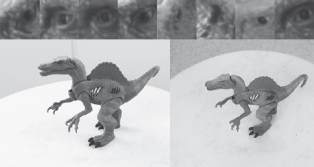
Using recognition methods, the mapping problem is converted into a classification problem [LEP 04]. The subjacent idea involves the use of a learning phase, using several images of a scene to “learn” the photometric appearance of the same 3D point from different viewpoints. This appearance database, is then used in the operational phase to map a point of interest onto a 3D point by seeking the elements in the database, which are most similar to that point [OZU 06]. Figure 15.1 illustrates this procedure: several images of a scene, from different viewpoints, have been taken. Points of interest are extracted and mapped in the images, and the set of corresponding 3D points is determined using a structure from motion type algorithm [AGA 09]. A point is therefore represented by a class containing the collection of patches taken from the 2D images in which it was detected. During the application phase, for each acquired image and each extracted point of interest x, we seek a class C such that P(x|C) is maximized, allowing the detected point to be associated with a 3D point.

Figure 15.1. Representation of a point by a collection of its aspects: the eye of the dinosaur is represented by the various appearances which it may take in a set of learning images

These methods have enjoyed considerable success in recent years. Unlike iterative tracking-type methods, they do not block in cases of failure, even if the recognition method fails for one of the images. As with all learning-based methods, however, difficulties arise if the viewpoints adopted in the operational phase are very different from those used in the learning phase. For this reason, other techniques, which aim to synthesize a large number of additional viewpoints, are often used to complement the learned database, via the application of affine or homographic distortions to learning images [HSI 10]. This method generates realistic views if the object is locally planar; in other cases, it only generates an approximation of reality. If a textured model of the object is available, it is also possible to generate realistic views using a rendering engine.

15.2.2.3. Choice of points of interest and real-time constraints

Methods may differ according to the type of points of interest and the classification methods used, and are driven by the need for real-time computation of the mapping phase. Point of interest detectors, which are not subject to certain transformation groups (similarity and affine) and of which scale-invariant feature transform (SIFT) and speeded-up robust features (SURF) are the best known examples, allow mapping of points seen from relatively different aspects. However, the descriptor is relatively large (128) and the calculation and mapping involved are slow, meaning it is hard to use with mobile architectures, although improvements to reduce descriptor size have been proposed, such as PCA-SIFT [KE 04]. More recently, faster computing detectors with smaller descriptors have emerged, including BRIEF [CAL 12]; BRIEF uses a binary descriptor, where each element is the result of an intensity comparison between two points of the patch. This descriptor may be implemented rapidly and compares favorably with SIFT and SURF in performance terms. However, it is subject to problems of rotation invariance. A new detector, Oriented FAST and Rotated BRIEF (ORB), has recently been released to correct these invariance faults [RUB 11].

15.2.3. Pose computation: principal PnP algorithms

In this section, we will focus on pose computation using perspective-n-point camera pose computation (PnP) methods, which calculate poses using n 2D/3D point correspondences (m_i, M_i), with known intrinsic parameters.

A number of articles have been published that consider pose computation based on a small number of exact correspondences (often from three to five). There is not always a single solution: the perspective-3-point camera pose computation (P3P) problem, with three corresponding points, generally possesses four solutions [FIS 81]. In cases with four points, some cases produce two or more solutions. However, the solution will be unique if the points are coplanar without co-linear point triplets [FIS 81].

15.2.3.1. Pose computation by minimization of reprojection error

In practice, we have access to a large number of mapped points and these points are subject to noise. It is not, therefore, useful to seek an exact solution; instead, we aim to estimate a solution using the least squares method to minimize the reprojection error for the point set [LOW 87]

where z is the application that transforms a homogeneous vector into a point with Cartesian coordinates (x/z, y/z) and dist is the application that calculates the Euclidean distance between two points. In this case, there is no direct solution to the minimization problem. For this reason, iterative minimization methods are generally applied, starting from an initial estimate. In practice, we often choose the calculated pose for the previous instant as the estimate, presuming, implicitly, that the movement of the camera is sufficiently smooth. For the initial solution, we use an exact solution obtained from a small number of points. This clearly does not guarantee that the method will converge, particularly if the camera is moving rapidly, something that occurs frequently in augmented reality when the user turns his or her head. For all of these algorithms, sensor data greatly facilitate pose computation by providing an initial estimate close to the optimum [ARO 06].

Certain methods also use approximations of the projection model [DEM 95] or abandon the orthogonality constraint of matrix R in order to facilitate convergence. However, these techniques still do not guarantee convergence. Other methods use multiple initializations, but are very costly. In a similar vein, the expansion of sampling techniques and particle filtering methods [ISA 96] has brought significant improvements in terms of the robustness of pose computation. The basic idea is to sample the distribution of the pose in the vicinity of the current estimation. In this way, we generate a set of potential poses, weighted in relation to reprojection error (the higher the weight, the lower the projection error). In this way, the pose can be calculated as a weighted mean of these particles. The sampling process is based on an a priori distribution (often a Gaussian distribution centered on the last estimation) or linked to knowledge of movement dynamics that allow us to predict pose in the current image [CHA 02, PUP 05]. The advantage of these methods is that they allow us to generate potential poses that are relatively distant from the current pose, thus accounting for non-smooth camera trajectories. The precision of these techniques clearly depends on the number of particles used, but they provide a considerable improvement in the robustness of pose computation in cases of sudden movement or occlusions in the sequence.

15.2.3.2. Direct pose computation methods

In recent years, the convergence difficulties present in iterative methods and the impossibility of mastering processing time have led to research concerning non-iterative pose computation solutions. The efficient perspective-n-point camera pose estimation (EPnP) [LEP 09] and direct least squares (DLS) [HES 11] algorithms are good examples of this.

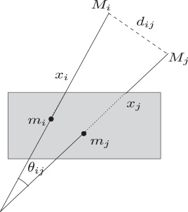
In most non-iterative methods, the objective is to express coordinates of 3D points in the camera frame by calculating the depth associated with each image point. A relationship exists linking the distances d_ij between points in the model, the depth of the points x_i in the image frame and the angle θ_ij between lines of sight. Using trigonometry (see Figure 15.2), we obtain The d_ij values are known from the model and, as the camera is calibrated, θ_ij may be calculated using the image points m_i and m_j. We thus obtain second-degree polynomial equations of which the unknown values are depth values in the camera frame [ANS 03]. Pose computation thus involves finding the rigid transformation that best aligns the points in the model expressed in the camera frame and those expressed in the general plane, for example using [UME 91]. Unfortunately, these methods are complex and do not take account of errors in extracted points.

Figure 15.2. Basic geometry involved in pose computation using corresponding points

The recent EPnP method [LEP 09] is based on the idea of expressing each 3D point as the weighted sum of four virtual points via barycentric coordinates. This weighting is the same whether the point is expressed in the general plane or the camera frame. For each pair (m_i, M_i), we may thus write two equations depending on the image point and the weightings, for which the unknown values are the coordinates of the four reference points expressed in the image frame. The concatenation of the equations for n observations allows us to estimate reference points using least squares, then the model points in the camera frame and finally the pose by aligning the two sets of points. The core of the algorithm involves the calculation of the coordinates of the four reference points, obtained by least squares resolution of a system of size 2n × 12 ( 2n × 9 if the points are coplanar), which may be carried out with a complexity in O(n).

One drawback of this type of method is that it does not consider noise in extracted points. The DLS approach [HES 11] tackles this problem and offers a method for finding all solutions of a least squares formulation of the PnP problem. In this approach, the rigid constraint that exists between the points expressed in the general plane and the camera frame is used to express the depth of points and the translation as a function of the rotation R. The least squares criterion minimizes the difference between the measured line of sight and the line of sight deduced from the model by the transformation [R, T], and is expressed as a fourth-degree polynomial in rotation parameters, providing third-degree optimality conditions with calculable roots. A non-optimized implantation produced using Matlab provided a time of around 15 ms with precision levels close to those produced by iterative methods (in cases of convergence).

The development of efficient initialization-free methods has enabled pose computation methods suited to augmented reality applications in which the need for re-initialization arises on a regular basis.

15.2.4. Pose computation and planar surfaces

Many applications of AR take place in urban or indoor environments that are often piecewise planar. In these cases, the scene is often described in terms of a computer-aided-design (CAD) model of the environment using a set of planar surfaces to construct the scene. Pose computation must then be based on correspondences between 3D and 2D faces. The basic notion used in this case is that of planar homography (see Figure 15.3). Let X be any point in a plane π of which the equation is given by n^tX + d = 0. The plane is observed by two cameras, of which the projection matrices are denoted by P and P′.We may presume that P = K[I,0] and P′ = K[R, T], within a change of frame. Let x and x′ be the homogeneous coordinates of the projections of point X by P and P^′. We can then easily demonstrate [HAR 00] that a linear transformation exists, 3 × 3 H, known as homography, such that x′ = Hx. This transformation is given by:

[15.2]

Figure 15.3. Plane-induced homography

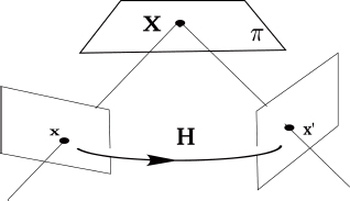
The linear transformation H may be calculated using at least four points in correspondence belonging to the same plane using a least squares type estimation. If the matrix of intrinsic parameters K is known, then knowledge of H allows us to write nine proportional equations, i.e. eight equations including the unknown values R and T. Representing a spatial rotation using three parameters (Euler’s angle, quaternions, etc.), we thus obtain eight equations with six unknown values, allowing us to calculate the relative movement between three positions. A linear solution to this problem can be found supposing (which is always possible) that the observed plane has the equation z = 0 [SIM 00]. The precision of the pose computation may be improved by using several planes [VIG 03]. A number of projects are currently underway with the aim of automatic acquisition of the plane equation in a scene for pose computation (see section 15.3). Certain approaches use the notion of dominant planes in urban environments and the extraction of points at infinity for the main directions in the scene [KOS 05]. Others use interactivity for precise reconstruction of planes in a scene [SIM 11].

15.3. Model acquisition

An overview of techniques used to reconstruct objects is given in Chapter 8 In this section, we will consider the generation of 3D models that may be used for real-time pose computation and the management of spatial (occlusions and collisions) and photometric interactions (shadows and light reflection) between the real and virtual worlds. We will consider scenes of varying sizes, from manufactured objects to urban landscapes.

15.3.1. Offline modeling

A point cloud associated with descriptors may be obtained using a structure from motion (SFM) algorithm. To do this, the scene for reconstruction must be filmed using a moving camera. Points of interest are detected and mapped between sequence images, and then recreated in 3D using binocular or multi-ocular stereovision techniques (see Chapter 7). Non-linear optimization is generally used to refine this initial solution, taking account of the global coherence of the 3D reconstruction in relation to the 2D points measured throughout the sequence. This step is known as bundle adjustment. Much has been written concerning SFM methods, the basics of which are covered by Hartley and Zisserman [HAR 00] and in an overview by Triggs et al. [TRI 00].

Denser point clouds can generally be obtained by combining image data with laser data. In [FRU 01], for example, two inexpensive 2D lasers and a camera, with precision-calibrated positions and relative orientations, were mounted onto a vehicle traveling through the streets of a town. One laser scanned buildings horizontally, the other laser scanned vertically. The point map produced by the horizontal scan was compared to aerial photographs and digital road maps to improve the precision of the obtained geometry.

The interest of point cloud models for AR, however, is limited for several reasons. First, positioning a 3D object in a point cloud requires calibration to within six degrees of freedom, which may be difficult in point clouds where the structural elements of a scene are difficult to identify. It is, however, easy to place an object on a surface of a model by forcing the vertical of the object to remain aligned with the normal of the surface, for example. Second, a surface model allows us to obtain a visibility map that is useful both in managing occlusions between the real and virtual world and for obtaining the primitives of the model that are visible at a given instant and may be used for pose computation. Finally, the calculation of shading and light reflections between real and virtual elements depends on the use of surface models.

Certain authors have considered the automatic detection of coplanar point groups in a point cloud [KOS 05], from which planar surfaces may be obtained. However, the proposed methods are generally unreliable for a number of reasons, discussed in [SIM 11]. Their use notably requires calibration of a number of parameters of which the optimal values are linked to the size of the scene and the context of application. A surface mesh may also be obtained by triangulating a point cloud. In [FRU 01], for example, a cloud is triangulated by connecting neighboring points under certain regularity constraints, and the images captured by a camera were used to texture the generated triangles. However, the meshes obtained using this type of procedures generally contain a number of holes and/or phantom triangles.

For this reason, it is more reliable to involve the user in segmenting point clouds to convert them into structured and/or textured surface models. The authors of [VAN 07] propose using point clouds as a basis for an interactive modeling of the scene. A mouse is used to trace polygons directly onto video images, which are then reconstructed in 3D for optimal adjustment to SFM-generated point groups. Straight lines or curves may then be traced onto these polygons for division or subdivision purposes. Autodesk ImageModeler is another example of a user interface that allows scene modeling based on a point cloud. The scene is represented by a set of elementary blocks (boxes, spheres, etc.) assembled by the user; the structural elements of these blocks (vertices, axes, etc.) are aligned with reconstructed points. In these two examples, textures taken from video images may be pasted onto the reconstructed model.

Other commercially available tools allow scenes to be modeled directly from images without passing through a point cloud. This allows a scene to be reconstructed from a single photograph, with the possibility of adding further photographs to provide a complete view of the scene. These programs use manually inserted parallelism and orthogonality constraints to obtain intrinsic parameters and the camera pose [WIL 02]. The 3D scene may then be modeled incrementally by the user, using an image as a visual support [OH 05]. Google SketchUp is one such program that uses this technique.

15.3.2. Online modeling

As AR spreads, it has become increasingly difficult to require inexperienced users to model their own environment before using an AR application. Currently, artificial markers [KAT 99] are generally used to avoid this stage, but the markers still need to be printed onto paper and the solution would not be appropriate for complex or large-scale environments (generally anything more than 10 times the size of the marker). Recent and current work has focused on circumventing the modeling phase, with environment acquisition taking place at the same time as positioning, or in a rapid initial phase requiring little user expertise. These approaches also enable what you see is what you get (WYSIWYG) environment modeling, avoiding postprocessing problems, and presents an interest for other contexts of use such as special effects in cinema, with high economic stakes at play.

For small-scale scenes (objects, work surfaces, etc.), visual simultaneous localization and mapping (SLAM)-type methods may be used [DAV 02, EAD 06, KLE 07]. These methods are based on the hypothesis of the camera being moved, allowing points identified in several images to be reconstructed using stereovision techniques. A Kalman filter [DAV 02] or a particle filter [EAD 06] is generally used to refine the 3D position of these points during the process. The 3D map may also be refined as a whole using bundle adjustment, an operation that may be carried out at a frequency lower than that of positioning, and using a different processor in order to respect the real-time constraint [KLE 07].

Positioning virtual objects in a 3D map is even harder in this context than in an offline situation. In [KLE 07], a dominant plane is calculated for placement of the virtual object, but this procedure is not suited to complex or multiplane environments. The authors of [PAN 09] propose “on-the-fly” transformation of a point cloud into a textured surface mesh. A Delaunay tetrahedrization is applied to the point cloud, followed by a probabilistic sculpture phase used to find the hollows in convex solids. This procedure is designed to reconstruct handheld objects, presented to the camera from different angles. It is not suited to use with non-manipulable scenes. Moreover, the reconstructed surface often contains faults (unfilled holes or parasite triangles) that may lead to strange visual effects when the model is used to manage occlusions.

The appearance of time-of-flight (TOF) cameras, particularly the relatively inexpensive Microsoft Kinect, has attracted strong interest from the AR community. The Kinect uses a structured light technique [FRE 08] to generate depth maps of a scene in real time, from which a discrete point cloud may be obtained. In [IZA 11], the iterative closest point (ICP) algorithm is used for real-time alignment of this initial cloud with new clouds obtained when the camera moves. This allows us to obtain a camera pose for each instant, and to supplement the initial point cloud with points that become visible as the camera moves. Unlike the 3D maps obtained using SLAM or by SFM, the point clouds generated in this way are very dense. Representing each 3D point by a voxel, we obtain a relatively precise volumetric model that can be used to manage occlusions and collisions between the real scene and virtual objects. This technique appears promising, but is currently limited to indoor scenes with a size limited by the camera range (around 3 m). Moreover, a volumetric representation in voxel form gives an understanding of the scene no better than that obtained using a point cloud.

In situ modeling methods have been proposed in response to this issue, allowing us to obtain a structured representation of the scene by modeling directly over the flow of video images obtained in real time. In [BUN 08], a poster is used to obtain camera poses until the reconstructed model is sufficiently rich to take over. While positioning is taking place, the user may designate a point in the current image (generally the apex of an object) using a mouse. When the camera moves, the epipolar line corresponding to this point is tracked, and the user may move the point along this line until it reaches the correct position for the current image. The polygons modeled in this way may be extruded to produce volumes. Once a sufficient number of edges have been modeled, contour-based tracking is used in the place of the poster for pose computation and the remaining modeling operations. This method is relatively inconvenient for the user, due to the use of the poster in the activation phase and the complexity of the interactions required to obtain a complete model.

Figure 15.4. In situ environment modeling using a method developed by the MAGRIT team. a) The walls and floor are targeted and captured through the camera, then reconstructed in real time using simple interactions. After a few seconds, a virtual scene (of simple palm trees, in this case) may be integrated into the modeled environment. A video showing these operations is available at www.loria.fr/˜gsimon/vc/blobs_outdoor.avi. b) Example of blobs obtained in the corridors at the Loria. These blobs can be used to easily position virtual objects in relation to the real scene

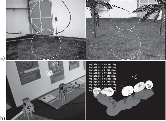
In [SIM 11], we proposed a paintbrush-type technique, more intuitive and less inconvenient, for in situ modeling of piecewise planar environments (objects, indoor scenes, urban environments, etc). The user “paints” visible faces of the model through a disk displayed in the middle of the video image (see Figure 15.4(a)). When the user presses a key, the disk is placed onto the face, then tracked in real time by mapping points of interest between consecutive images and robust homography calculation. Disks posed on the same phase are concatenated to form convex polygons known as blobs. When two blobs are tracked on secant planes, the image of the intersection of the two planes is determined using a particle filter with geometric and photometric constraints. The user may then visually validate the obtained line, or restart the filter if the trace does not converge or converges to an imprecise solution. Once the image of the intersection has been obtained, the equations of the planes corresponding to the two blobs are calculated, taking into account this information and the geometric constraints linked to the movement of the camera. Using this method, we do not obtain an exhaustive representation of the environment or the object, but textured 3D blobs that allow pose computation and facilitate the positioning of virtual objects (see Figure 15.4(b)).

15.4. Conclusion

AR has made significant progress in recent years, allowing us to envisage increasingly complex applications. This progress is due to the combination of several factors:

However, few applications are currently able to operate in large-scale environments, particularly outdoors. In these contexts, changes may occur between the moment the scene is acquired and the time the application is used, presenting major difficulties. These modifications may be spatial (changes in an urban environment, traffic and pedestrians), and may concern the ambient lighting or climatic conditions (rain, snow, etc.) creating considerable differences between the model and the current scene and making the model/image mapping stage much more complex. Another significant difficulty in applications requiring high levels of realism lies in the photometric coherence of the real/virtual mix. The problem of shading or relighting is on the border between the domains of computer vision and graphical information technology; it is particularly complex in the case of natural light, and is the subject of current research.

15.5. Bibliography

[AGA 09] AGARWAL S., SNAVELY N., SIMON I., et al., “Building rome in a day”, Proceedings of the 9th International Conference on Computer Vision, Kyoto, Japon, October 2009.

[ANS 03] ANSAR A., DANIILIDIS K., “Linear pose estimation from points or lines”, IEEE Transactions Pattern Analysis and Machine Intelligence, vol. 25, pp. 578–589, 2003.

[ARO 06] ARON M., SIMON G., BERGER M.-O., “Use of inertial sensors to support video tracking”, Computer Animation and Virtual Worlds, vol. 18, pp. 57–68, 2006.

[AZU 01] AZUMA R.T., BAILLOT Y., BEHRINGER R., et al., “Recent advances in augmented reality”, Computer Grahics Applications, vol. 21, pp. 34–47, December 2001.

[BUN 08] BUNNUN P., MAYOL-CUEVAS W.W., “OutlinAR: an assisted interactive model building system with reduced computational effort”, IEEE/ACM International Symposium on Mixed and Augmented Reality, IEEE Computer Society, Los Alamitos, CA, pp. 61–64, 2008.

[CAL 12] CALONDER M., LEPETIT V., OZUYSAL M., et al., “BRIEF: computing a local binary descriptor very fast”, IEEE Transactions on Pattern Analysis and Machine Intelligence, vol. 34, pp. 1281–1298, 2012.

[CHA 02] CHANG P., HEBERT M., “Robust tracking and structure from motion through sampling based uncertainty representation”, Proceedings of ICRA ’02, Washington, May 2002.

[DAV 02] DAVISON A.J., MURRAY D.W., “Simultaneous localization and map-building using active vision”, IEEE Transactions on PAMI, vol. 24, pp. 865–880, 2002.

[DEM 95] DEMENTHON D., DAVIS L., “Model based object pose in 25 lines of code”, International Journal of Computer Vision, vol. 15, pp. 123–141, 1995.

[DRU 99] DRUMMOND T., CIPOLLA R., “Real-time tracking of complex structures with on-line camera calibration”, Proceedings of the British Machine Vision Conference, BMVC 99, Nottingham, 1999.

[EAD 06] EADE E., DRUMMOND T., “Scalable monocular SLAM”, Proceedings of the 2006 IEEE Computer Society Conference on Computer Vision and Pattern Recognition, IEEE Computer Society, Washington, DC, pp. 469–476, 2006.

[FIS 81] FISCHLER M.A., BOLLES R.C., “Random sample consensus: a paradigm for model fitting with applications to image analysis and automated cartography”, Commununications of the ACM, vol. 24, no. 6, pp. 381–395, June 1981.

[FRE 08] FREEDMAN B., SHPUNT A., MACHLINE M., et al., “Depth mapping using projected patterns”, Patent Application, 10 2008. WO 2008/120217 A2, 2008.

[FRU 01] FRUH C., ZAKHOR A., “3D model generation for cities using aerial photographs and ground level laser scans”, Proceedings of the 2001 IEEE Computer Society Conference on Computer Vision and Pattern Recognition, 2001, CVPR 2001, vol. 2, pp. II-31–II-38, 2001.

[HAR 00] HARTLEY R.I., ZISSERMAN A., Multiple View Geometry in Computer Vision, Cambridge University Press, 2000.

[HES 11] HESCH J.A., ROUMELIOTIS S.I., “A direct least-squares (DLS) method for PnP”, International Conference on Computer Vision, Barcelona, pp. 383–390, 2011.

[HSI 10] HSIAO E., COLLET ROMEA A., HEBERT M., “Making specific features less discriminative to improve point-based 3D object recognition”, IEEE Conference on Computer Vision and Pattern Recognition (CVPR), San Francisco, June 2010.

[HUB 81] HUBER P.J., Robust Statistics, Wiley, New York, 1981.

[ISA 96] ISARD M., BLAKE A., “Contour tracking by stochastic propagation of conditional density”, Proceedings of the 4th European Conference on Computer Vision, Cambridge, UK, vol. 1064, pp. 343–356, 1996.

[IZA 11] IZADI S., KIM D., HILLIGES O., et al., “Kinect-fusion: real-time 3D reconstruction and interaction using a moving depth camera”, ACM Symposium on User Interface Software and Technology, Santa Barbara, USA, pp. 559–568, 2011.

[KAT 99] KATO H., BILLINGHURST M., “Marker tracking and HMD calibration for a video-based augmented reality conferencing system”, Proceedings of the 2nd International Workshop on Augmented Reality, San Francisco, CA, 1999.

[KE 04] KE Y., SUKTHANKAR R., “PCA-SIFT: A more distinctive representation for local image descriptors”, 2012 IEEE Conference on Computer Vision and Pattern Recognition, IEEE Computer Society, vol. 2, pp. 506–513, 2004.

[KLE 07] KLEIN G., MURRAY D., “Parallel tracking and mapping for small AR workspaces”, Proceeding of the 6th IEEE and ACM International Symposium on Mixed and Augmented Reality (ISMAR’07), Nara, Japan, November 2007.

[KOL 92] KOLLER D., DANIILIDIS K., NAGEL H.H., “Model-based object tracking in traffic scenes”, Proceedings of the 2nd European Conference on Computer Vision, Santa Margherita Ligure, Italy, vol. 588, pp. 437–452, 7 October, 1992.

[KOS 05] KOSECKA J., ZHANG W., “Extraction, matching and pose recovery based on dominant rectangular structures”, Computer Vision and Image Understanding, vol. 100, no. 3, pp. 274–293, 2005.

[LEP 04] LEPETIT V., PILET J., FUA P., “Point matching as a classification problem for fast and robust object pose estimation”, Proceedings of IEEE Conference on Computer Vision and Pattern Recognition, Washington, DC, pp. 244–250, 2004.

[LEP 05] LEPETIT V., FUA P., “Monocular model-based 3D tracking of rigid objects: a survey”, Foundations and Trends in Computer Graphics and Vision, vol. 1, no. 1, pp. 1–89, 2005.

[LEP 09] LEPETIT V., MORENO-NOGUER F., FUA P., “EPnP: an accurate O(n) solution to the PnP problem”, International Journal of Computer Vision, vol. 81, no. 2, pp. 155–166, February 2009.

[LOW 87] LOWE D.G., “Three-dimensional object recognition from single two-dimensional images”, Artificial Intelligence, vol. 31, pp. 355–395, 1987.

[OH 05] OH J., STUERZLINGER W., DANAHY J., “Comparing SESAME and sketching on paper for conceptual 3D Design”, EUROGRAPHICS Workshop on Sketch-Based Interfaces and Modeling, Konstanz, Germany, 2005.

[OZU 06] OZUYSAL M., LEPETIT V., FLEURET F., et al., “Feature harvesting for tracking-by-detection”, Proceedings of European Conference on Computer Vision, Graz, Austria, 2006.

[PAN 09] PAN Q., REITMAYR G., DRUMMOND T., “ProFORMA: probabilistic feature-based on-line rapid model acquisition”, Proceedings of the 20th British Machine Vision Conference (BMVC), London, September 2009.

[PUP 05] PUPILLI M., CALWAY A., “Real-time camera tracking using a particle filter”, Proceedings of British Machine Vision Conference, British Machine Vision Association 2009, pp. 519–528, 2005.

[RUB 11] RUBLEE E., RABAUD V., KONOLIGE K., et al., “ORB: an efficient alternative to SIFT or SURF”, International Conference on Computer Vision (ICCV), Barcelona, Spain, pp. 2564–2571, 2011.

[SIM 98] SIMON G., BERGER M.-O., “A two-stage robust statistical method for temporal registration from features of various type”, Proceedings of the 6th International Conference on Computer Vision, Bombay, India, pp. 261–266, 1998.

[SIM 00] SIMON G., FITZGIBBON A., ZISSERMAN A., “Markerless tracking using planar structures in the scene”, Proceedings of International Symposium on Augmented Reality, Darmstadt, Germany, pp. 120–128, October 2000.

[SIM 11] SIMON G., BERGER M.-O., “Interactive building and augmentation of piecewise planar environments using the intersection lines”, The Visual Computer, vol. 27, no. 9, pp. 827–841, February 2011.

[STE 99] STEWART C.V., “Robust parameter estimation in computer vision”, SIAM Reviews, vol. 41, pp. 513–537, 1999.

[TRI 00] TRIGGS B., MCLAUCHLAN P., HARTLEY R., et al., “Bundle adjustment – a modern synthesis”, Vision Algorithms: Theory and Practice, LNCS, vol. 1883, pp. 298–375, 2000.

[UME 91] UMEYAMA S., “Least-squares estimation of transformation parameters between two point patterns”, IEEE Transactions on Pattern Analysis and Machine Intelligence, vol. 13, pp. 376–380, 1991.

[VAN 07] VAN DEN HENGEL A., DICK A., THORMÄHLEN T., et al., “Video Trace: rapid interactive scene modelling from video”, ACM SIGGRAPH 2007 Papers, ACM New York, NY, USA, p. 86–91, 2007.

[VIG 03] VIGUERAS F., BERGER M.-O., SIMON G., “Iterative multi-planar camera calibration: improving stability using model selection”, Vision, Video and Graphics (VVG ’03), Bath, UK, July 2003.

[WIL 02] WILCZKOWIAK M., BOYER E., STURM P., “3D modeling using geometric constraints: a parallelepiped based approach”, 7th European Conference on Computer Vision (ECCV ’02), vol. 4, Springer-Verlag, Copenhagen, Denmark, pp. 221–237, 2002.

[ZHA 97] ZHANG Z., “Parameter estimation techniques; a tutorial with application to conic fitting”, Image and Vision Computing Journal, vol. 15, no. 1, pp. 59–76, 1997.

Chapter written by Gilles SIMON and Marie-Odile BERGER.