Chapter 19

3D HDR Images and Videos: Acquisition and Restitution

19.1. Introduction

The human eye is able to perceive up to 10 orders of magnitude of light intensity (10¹⁰ cd m⁻²), but only 5 simultaneously (see [FER 01] and Chapter 2). This order of magnitude is reduced to 2 when displaying images on standard screens. Images acquired up to now, known as low dynamic range (LDR) images, contain a limited range of light intensities. This restriction is highlighted in scenes involving back lighting, for example. For this reason, the development of images with high color dynamics, or high dynamic range (HDR), is increasingly important.

This type of image has recently been the subject of considerable research effort, focusing on acquisition, storage, display and use. Specific HDR cameras already exist, but are either still at the experimental stage or too costly. Methodologies have been established to compensate for the absence of specific material. An introduction to HDR images and classic acquisition methods is presented in Chapter 2, in which we see that static image capture has been the subject of particular attention. Current sensors allow us to acquire and directly store a wider dynamic range of colors (up to 16 bits for still cameras). HDR video has recently attracted much attention, but video sensors remain limited in terms of color intensity ranges (mainly represented in 12 bits). For now, it is difficult to transmit and store HDR video data in the absence of effective formats. The domain of HDR video is also relatively confidential. The number of known solutions for acquisition is very limited, as we will see in this chapter. For our purposes, the phrase “3D video” will refer to multiscopic video content (see Chapter 4).

This chapter is divided into two main sections, concerning acquisition and rendering, respectively. In section 19.2, we provide a classification of acquisition methods based on the domain in question, organized according to criteria: number of views in the scene, simultaneous or spread acquisition, acquisition of a static scene or a scene with variable representations over time. As no display technology currently permits HDR rendering, in section 19.3, we consider the possibilities of adapting existing technologies.

19.2. HDR and 3D acquisition

As we saw in Chapter 2, multiplying viewpoints during acquisition gives us the immediate ability to generate depth perception. Consequently, if we have hardware capable of native HDR data acquisition for a scene and repeat acquisition from several view points, it becomes possible to directly operate 3D HDR capture. This repetition might be obtained by moving or duplicating hardware, allowing simultaneous capture of different points of view and thus enabling HDR 3D video capture.

Unfortunately, little HDR-enabled hardware is currently available, and existing hardware is not suited to HDR video capture. Spheron¹ has developed panoramic HDR view capture equipment and an HDR video camera, although the latter is still at prototype stage and considerable quantities of data are involved. Weiss² offers a fully automated device, the Civetta, allowing acquisition of spherical HDR images over 360° with a resolution of 100 megapixels.

The current impossibility of obtaining native HDR data in the context of multi-viewpoint acquisition means we must use an HDR value estimation method to produce 3D HDR images. Methods for obtaining HDR images using LDR capture materials consist of combining several exposures of the same scene in order to conserve [AGG 04, MER 07] or estimate [DEB 97, MAN 95] the best brightness values for each zone in the image. The simultaneous manipulation of several images requires data to be calibrated both geometrically and colorimetrically. The level of precision used in this calibration phase varies between methods. In certain cases, we must estimate and apply the inverse response curve of the camera (see Chapter 2).

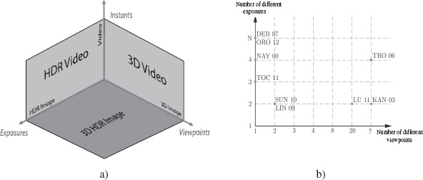
These methods, using multiple exposures, present strong analogies with the use of multiple viewpoints of the same scene when acquiring depth, or the acquisition of several instants of a dynamic scene to produce video. These analogies are shown in Figure 19.1(a), where 3D HDR video methods are divided using three axes: one corresponding to different exposures, a second to different viewpoints and a third to different instants. Note that the origin of these axes is not set at 0, but at 1: one exposition, one viewpoint and one instant. Each of the axes defines a specific type of acquisition: HDR images, 3D images and video. By choosing two axes, we create a plane showing other specific types of acquisition: HDR video, 3D video or 3D HDR images. Finally, the whole space (three axes) corresponds to 3D HDR video.

We will use this division into 1D and 2D subspaces to present different models described in literature on the subject. We will consider only one 1D subspace, HDR images, as the others are well known (videos) or covered elsewhere in this book (3D images). The same applies to the 2D subspace covering 3D video. We will, however, specify methods for the other 2D subspaces: 3D HDR imaging and HDR video. We will finish by discussing the possibility of extending some of these methods to the whole space, adding one or two dimensions in order to obtain 3D HDR video.

The methods presented in this chapter are classified in Figure 19.1(b) according to the number of viewpoints and the number of different exposures used during acquisition to construct HDR data. Section 19.2.1 presents methods that aim to acquire images with a single camera. Section 19.2.2 discusses a method that allows the acquisition of HDR video. In section 19.2.3, we will consider methods involving 3D HDR content.

For any space, the HDR reconstruction methods considered in this chapter mostly follow the acquisition pattern illustrated in Figure 19.2, divided into three stages. In the first stage, a series of LDR images are obtained with different exposures. Stage 2 consists of pixel mapping, followed by stage 3, which uses the HDR value reconstruction algorithm. The number n of LDR input images and the number of HDR output images vary depending on the chosen method. Typically, in the 1D subspace, the viewpoint will be the same for all images I_k and a single image, E, will be generated. In the HDR video 2D subspace, there will be as many generated images E_k as there are images in the final video sequence. Images I_k will vary in terms of viewpoint and exposure, and their number will not necessarily be the same as the number of generated images E_k. In the 3D HDR image subspace, the images I_k will represent the same content, but from different exposures and points of view. Generally, the number of generated HDR images E_k will be the same as the number of input images I_k. Similarly, the mapping process varies based on the input data I_k and the HDR reconstruction objectives. The mapping process consists of aligning images if the viewpoint and content are the same I_k, data recalibration if the viewpoint is the same or similar but the content is different and correspondence mapping if the content is the same but the viewpoint differs.

19.2.1. 1D subspace: HDR images

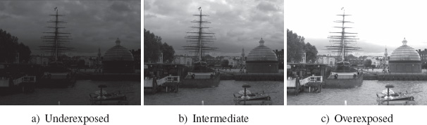
Numerous studies have considered the reconstruction of HDR values based on the acquisition of several images with different exposures from the same viewpoint [DEB 97, MAN 95, MIT 99]. Other approaches are mentioned in [LOS 10] and [REI 10]. Certain photographic cameras have an autobracketing function, which allows users to acquire images with different exposures using an automatic procedure, e.g. underexposed, normally exposed and overexposed views as shown in Figure 19.3. Depending on the camera, up to nine differently exposed images may be acquired using this method (see Chapter 2). In cases where this function is not available, the exposure time may be adjusted manually in order to acquire the required number of images of a scene. Whatever method is chosen, use of a tripod and a timer (or remote control) is recommended in order to stabilize the device and minimize the risk of shifts between images, leading to better results.

As we have already seen, in the absence of native HDR acquisition methods, we need to use an HDR value estimation method. We will presume that we have access to a series of images taken from the same viewpoint, but with different exposures. These images are perfectly aligned, and a point of the scene is projected at the same pixel coordinates (i, j) for all images. We have an additional set of information concerning the amount of light, recorded by the camera, coming from this point. The estimation of the HDR value for this point consists of combining these sets of information. A common method used for this operation was developed by Debevec and Malik [DEB 97], and consists of calculating a weighted average E(i, j) (see equation [19.1]) of luminance values (HDR values) for the three color components for corresponding pixels in each image, with a weighting function w based on the pixel saturation level:

[19.1]

where N is the total number of images, I_k(i, j) is the color value of the pixel with coordinates (i, j) in image I_k acquired with an exposure time Δt_k and f⁻¹ is the inverse function of the camera response (see Chapter 2). This function may be ignored if RAW data are used directly, in which case the data may be considered to be linear.

Different weighting functions w have been proposed to take under- or overexposed pixels into account. A state of the art of these methods is presented by Granados et al. [GRA 10]; each method is differentiated by the type of formula applied. A graphical representation of the performance of these methods is also given, showing that their method and the method put forward by Mitsunaga and Nayar [MIT 99] produce the best results.

In [AGU 12], the method put forward by Granados et al., based on the maximum likelihood estimation [GRA 10], was also shown to produce the best results. Aguerrebere et al. [AGU 12] proposed a new weighting function, allowing all pixels, including saturated pixels, to be taken into account; according to the authors, these pixels contain useful information for HDR data estimations.

Even when a tripod is used to guarantee acquisition stability, the fact that acquisitions occur at successive instants introduces sensitivity to the presence of moving objects or persons, which (or who) will be in a different position in each image. Several methods have been developed to detect and take this movement into account [JAC 08, GAL 09, GRA 08, GRO 06, SAN 04, WAR 03]. In the same context, Khan et al. [KHA 06] and Pedone et al. [PED 08] have calculated the probability that a pixel will belong to a static part of the image. Only Orozco et al. [ORO 12] have obtained an HDR value for all pixels, even those affected by movement, using mutual information or the normalized cross-correlation (NCC).

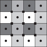
Instead of multiplying view captures to obtain different exposures, another method consists of acquiring sets of pixels at different exposures in a single operation. Nayar and Mitsunaga [NAY 00] adapted a camera by fixing an optical mask, such as the one shown in Figure 19.4, adjacent to a conventional image detector array. This filter permits the acquisition of four different exposures of the same image, distributed regularly by groups of four pixels. The final HDR image is then constructed either by aggregation or by interpolation. The first method allows calculation of the mean value of four neighboring pixels, a value which is then assigned to the center of the group of pixels. Considering an original image of size N × N, using this method, the final image will be of size (N − 1) × (N − 1). In the second case, the pixels in the image are divided into two categories: on-grid points (black disks in Figure 19.4) corresponding to the center of pixels, and off-grid points (black squares in Figure 19.4) corresponding to the intersection point of four pixels. This gives us a value for each pixel center, so there is no loss in resolution. For each of the two groups, saturated pixels are distinguished from non-saturated pixels. First, the off-grid points are calculated from the non-saturated on-grid points, then all of the off-grid points are interpolated to obtain on-grid points.

19.2.2. 2D subspace: HDR videos

Several exposures and several instants are required to obtain HDR video. According to an idea put forward by Kang et al. [KAN 03], we may use different acquisition instants to obtain different exposures. In this method, the acquisition procedure alternates long and short exposure times from one image to the next. Reconstructed HDR values for a given image at time t_i are obtained using data from the image at t_i−1 and the image at t_i+1. In this context, pixel shifts may be due to a change in camera viewpoint and to changes in the content of a scene from one instant to the next. Kang et al.’s pixel mapping method is based on the use of optical flow to estimate the movement of a pixel from one image to the next, an estimation that is then refined using homography. Once these displacements have been correctly estimated, it becomes possible to combine the values of corresponding pixels to obtain an HDR image. The results may include artifacts when there is rapid movement, as acquisition is limited to 15 images per second because of the alternating exposure times and optical flow is efficient mostly in a near neighborhood. Another limiting factor is the reduced number of exposure times available when reconstructing an image.

HDR video acquisition is also possible by obtaining several exposures for each instant, as with Nayar and Mitsunaga’s optical filter [NAY 00] (see section 19.2.1). Tocci et al. [TOC 11] have developed another type of camera, using three sensors that receive a different percentage of the incident light by prism diffraction. Three images with different exposures are thus obtained for a single capture, with no shifts between images. Unlike Debevec and Malik’s method [DEB 97], which used all pixel values from different acquired images, in this case only the pixels with the highest exposure are taken into account. The pixel at the same position in the image with lower exposure is only taken into account when a pixel is saturated, reducing the quantity of data to manage in lower exposure images, generally affected by different sensor-related noise.

19.2.3. 2D subspace: 3D HDR images

All HDR image acquisition techniques may be extended to 3D by multiplying viewpoints. In this way, we obtain multiple exposures for each viewpoint, and thus, after estimation, an HDR image for each viewpoint. These are recombined during restitution to obtain a 3D HDR image. Clearly, while this principle is viable, the number of images to acquire makes it costly, except when using the systems developed by Nayar and Mitsunaga [NAY 00] or Tocci et al. [TOC 11], which only require a single capture for multiple exposures. For standard capture devices, one way of improving this situation would be to vary exposure at the same time as the viewpoint, thus obtaining one exposure per viewpoint. However, this solution includes problems with luminance matching, as a point in the scene will not be projected onto the same pixel in different images. Mapping therefore needs to be carried out before estimating brightness values. In this section, we consider the matching methods used in HDR reconstruction.

19.2.3.1. Stereo matching for HDR reconstruction

Many different methods exist for pixel matching. In this particular context, the input data contain a variety of intensity values. Dark, or saturated, zones have poor or erroneous data that vary across the sequence of considered images. Moreover, if this sequence is captured using several lenses, the data will have a higher degree of variability. We therefore need to establish a procedure for calibrating data to make it consistent (see section 19.2.3.2) and adapt or propose new matching algorithms. In this section, we explore four recent methods for tackling this problem.

Lin and Chang [LIN 09] aimed to match pixels contained in two images acquired from different viewpoints with different exposures, supplied by Middlebury³. To do this, they applied Sun et al.’s algorithm [SUN 03], based on belief propagation, after modifying the images to obtain a shared exposure time. This algorithm establishes a correspondence between pixels using three Markov random fields, corresponding, respectively, to three important problems that must be addressed during the matching phase: disparities, discontinuities and occlusions in the different images. While Lin and Chang [LIN 09] only used one set of stereoscopic data, Sun et al.’s method [SUN 03] has also been tested on multiscopic image sets (5 and 11 viewpoints), where an additional cost function is minimized in order to match pixels with the lowest cost.

Sun et al. [SUN 10] also proposed a solution for matching pixels taken from stereoscopic images acquired with two exposure times (Middlebury images³). As we saw in Chapter 7, different similarity measurements may be taken into account for matching purposes. In this case, the authors chose to use NCC, which is invariant to exposure changes. Different similarity measurements have been compared for mapping pixels taken from images with different exposures [BLE 08, ORO 12], and the NCC method currently produces the best results. Its invariance to changes in brightness under certain conditions was demonstrated by Troccoli et al. [TRO 06], who used it to improve results obtained using Kang and Szeliski’s method [KAN 04]. To do this, two matching operations were carried out, the first with NCC and the second with the sum of square differences (SSD) in the luminance space to refine initial results. This method used N viewpoints and four different exposures.

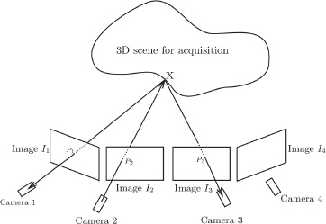
Lu et al. [LU 11] considered 3D HDR reconstruction and have not directly addressed the production of 3D HDR images. They proposed the use of projection to assist matching, as shown in Figure 19.5, using a dome of 20 cameras to obtain images with two exposures simultaneously. Ten cameras acquired images with one exposure time and the ten others with the second exposure time. If we know pixel P₂ in image I₂, its projection X in the scene to acquire is also known (the point belongs to the optical center/pixel line). By inverse projection onto images acquired by other cameras, it is possible to find the points corresponding to this 3D point in all images in which it features. Points P₁ and P₃ thus correspond to point P₂ in images I₁ and I₃. The zero normalized cross-correlation (ZNCC) is then used to limit correspondences and improve their coherency.

Bonnard et al. [BON 12] proposed an original approach, extending a purely 3D acquisition method to the context of HDR. The camera is presented in Chapter 3 and is built so that the objectives are in decentered parallel optical geometry, thus simplifying matching algorithms. In this case, Niquin et al.’s method [NIQ 10] was used for the matching stage in which pixels were matched by color similarity in a neighborhood and on the same line. The acquisition of different exposure times is simulated by applying a neutral density filter to each lens. Three filter pairs are selected: 0.3, 0.6 and 0.9, permitting simultaneous acquisition of eight images with four different exposures. This method is sensitive to data calibration, as the matching technique is based on a color similarity calculation. Calibration is difficult as each lens is independent.

Of the four methods presented above, the best results have been produced by Sun et al.’s approach [SUN 10]. These results are comparable to those obtained by Lin and Chang [LIN 09] due to the use of the same image set. Lu et al.’s method [LU 11] cannot be directly compared with the two methods above, as the authors wished to reconstruct HDR textures. Nevertheless, their results show the possibility of reading the text contained within an image using HDR rendering, something which cannot be done in an LDR context. For Bonnard et al.’s method, the artifacts that appear during the matching phase demonstrate reconstruction errors in different HDR images.

19.2.3.2. Discussion of color data consistency

The brightness values for each pixel come into play when estimating their value for the final HDR image, but they may also be necessary to bring all different exposures into the same space. This stage is essential in matching methods which have not been designed for images with different exposures.

Two cases are possible: if a single device is used (and moved to obtain different viewpoints), a single response curve may be used to linearize data; if several devices, or several sensors on the same device are used, then a response curve must be estimated for each device. The discussed method works with a single exposure time per device, so the response curve may only be estimated at the pre-processing stage. For this reason, simplifications are often used: for instance, Lu et al. [LU 11] considered that the set of camera sensors were of the same type and subject to the same calibration, and therefore reacted to light in the same manner. A single response curve was then calculated for one view, and used to retrieve luminance space values for all of the pixels of the images acquired by the different cameras. This hypothesis was not verified for Bonnard et al. [BON 12].

A final point to consider is that the estimation of a response curve requires us to operate on pixels representing the same 3D point in a scene, so preliminary matching may be needed to estimate the response curve. This curve may then be used for a second matching phase used in HDR calculations [LIN 09, SUN 10].

19.2.4. Extension to the whole space: 3D HDR videos

To date, no method has been developed to generate a 3D HDR video flow. However, an extension of 3D HDR imaging methods for video may be envisaged. These methods use a minimum of two images acquired with different exposure times. For video, the simultaneous acquisition of images for each filmed frame must be guaranteed, and problems generated by different exposure times (for example non-identical blurring of a fast-moving object) would need to be solved.

Kang et al. [KAN 03] encountered this problem in developing their HDR video method, a method that might be extended to produce 3D HDR video using N viewpoints and two exposures, by multiplying the number of cameras and ensuring synchronization. This procedure could also be used to extend Tocci et al.’s method [TOC 11] (prism cameras) or the Nayar and Mitsunaga method [NAY 00] (with a modified camera filter). These last two methods pose fewer problems as different exposures are obtained for each image.

The final question to consider concerns the performance of these envisaged methods. Although video postprocessing is generally accepted as a necessary step, the ultimate aim of video is live retransmission. This presents a considerable challenge, as, in addition to matching operations, HDR values need to be estimated for all of the images used in producing a 3D image. For the moment, this goal is out of reach. In addition to the problems discussed above, the restitution phase itself can require specific calculations (see section 19.3).

19.3. 3D HDR restitution

Visualizing 3D HDR content is problematic, as none of the displays currently available are able to present both HDR and 3D content. In this section, we consider a compromise based on available technologies and algorithms. We propose two approaches, which aim to combine the benefits of HDR and 3D display, based particularly on stereoscopic and multiscopic display techniques. HDR data may either be transformed for a non-HDR-dedicated display (section 19.3.1), or displayed directly in stereo on an HDR-dedicated display (section 19.3.2).

19.3.1. Rendering on a 3D-dedicated display

Screens allowing 3D content to be displayed with or without glasses have existed for a few years and are discussed in further detail in Chapter 14, but do not allow visualization of HDR content. We therefore need to adapt generated 3D HDR content to show on a standard display. Tone mapping algorithms may be applied [TUM 93] to convert an HDR image into a 24 bit RGB image, enabling perceptual preservation of contrasts in the image. A variety of tone mapping algorithms have been proposed, prioritizing either human perception, the quality of color rendering or computing efficiency; a list of these methods is presented in [BAN 11, DEV 02]. An evaluation method for these tone mapping operators is given in [CAD 08].

A single image may be rendered after applying algorithms such as those proposed by Reinhard et al. [REI 05] or Fattal et al. [FAT 02]. However, in our case, tone mapping algorithms must operate both on HDR and multiview video content. Certain tone mapping operators have already been proposed for HDR video by Drago et al. [DRA 03] and Kang et al. [KAN 03]. In this case, temporal consistency must be maintained for the operator to consider the images as a sequence rather than independently, based on calculations carried out for previous images. Yang et al. [YAN 12] propose an original approach to tone mapping, using the properties of human binocular vision and stereoscopic rendering systems: different tone mapping is applied for the left and right eyes, and the human visual system uses this information to recreate an image with a higher dynamic range.

None of the algorithms developed to date is suited to both multiview and HDR video content. Most tone mapping operators use global data to obtain a perceptual optimization of the values to display. If we simply apply existing algorithms, the chosen operations may be different for distinct viewpoints, leading to visual inconsistency when all views are displayed simultaneously. The point at which the tone mapping operator is applied also requires consideration: before data processing for 3D display (choice of views and/or interleaving) or afterwards.

19.3.2. Displaying on an HDR-dedicated screen

The first HDR display was proposed by Heidrich et al. [SEE 04]. This display allowed the contrast relationship to be extended to 50,000:1 (compared to 300:1 for standard screens at the time). This notably involved a maximum brightness of 8,500 cd m⁻². A commercial version of this screen was offered by BrightSide, a company bought out by Dolby Canada⁴. The type of screens available has changed considerably; they are now available as light-emitting diode (LED)-based flat screens, commercialized by Sim2⁵. Current image technology consists of storing each color component in 16 bits, with American national standards institute (ANSI) contrast of 20,000:1 and luminance of 4,000 cd m⁻². This corresponds to a luminance spectrum over five orders of magnitude, as opposed to three for current liquid-crystal display (LCD) screens. One specificity of the Sim2 screen is the representation of total black. Other LED-based screens also increase perceived brightness, but this remains lower than the values offered by the Sim2 screen.

For a display frequency suitable for stereo, it is possible to send an HDR image flow reduced to the format accepted by the display, alternating right and left views and using active shutter glasses to create depth perception. The influence of the opacity of these glasses on perceived brightness remains to be measured.

19.4. Conclusion

In this chapter, we have presented methods used to extend the interval of color intensities to 3D video. These approaches are based on the reconstruction of HDR values. Although there is currently no stable approach for 3D HDR video generation, we have seen that advances have been made in complementary directions in multiscopic HDR imagery and in HDR video. We have seen that, while HDR data are popular, they cannot yet be rendered with the whole range of intensity used in their creation. Current display procedures may be adapted to provide better data display on 3D or HDR screens, but no procedure has been validated to date.

The storage of 3D HDR videos also needs to be considered. The standard formats used to store HDR images are listed in [REI 10]. The OpenEXR format has been adapted for HDR video, but was not intrinsically designed for this use. An HDR video format based on MPEG-4 has been proposed by Mantiuk et al. [MAN 04]. The use of standard formats might lead to faster adoption of HDR data in the industrial domain. The first approach has recently been put forward for compressing stereo and HDR data [SEL 12], which is compatible with standard formats. Given the speed of progress in HDR imaging, display and storage methods for 3D HDR data are likely to emerge in the near future.

This domain is still highly experimental but is expanding rapidly. The remaining issues are mostly technological, with a need for new capture devices, and algorithmic, requiring better data calibration and reliable matching. HDR reconstruction should tend toward better noise control and the conservation of consistency in reconstructed data in terms of space and time. Finally, live transmission will only be possible if both technical equipment and data processing operate in real time, and when an operational, standardized compression, transmission and display format becomes available.

19.5. Bibliography

[AGG 04] AGGARWAL M., AHUJA N., “Split aperture imaging for high dynamic range”, International Journal of Computer Vision, vol. 58, pp. 7–17, 2004.

[AGU 12] AGUERREBERE C., DELON J., GOUSSEAU Y., et al., Best algorithms for HDR image generation. A study of performance bounds, Technical report, 2012.

[BAN 11] BANTERLE F., ARTUSI A., DEBATTISTA K., et al., Advanced High Dynamic Range Imaging: Theory and Practice, AK Peters (CRC Press), Natick, MA, 2011.

[BLE 08] BLEYER M., CHAMBON S., POPPE U., et al., “Evaluation of different methods for using colour information in global stereo matching approaches”, in CHEN J., JIANG J., FÖRSTNER W. (eds), Congress of the International Society for Photogrammetry and Remote Sensing, vol. XXXVII, Part B3a, Beijing, China, pp. 415–420, July 2008.

[BON 12] BONNARD J., LOSCOS C., VALETTE G., et al., “High-dynamic range video acquisition with a multiview camera”, Proceedings of SPIE Optics, Photonics, and Digital Technologies for Multimedia Applications II, SPIC, vol. 8436, no. 1, p. 84360A, 2012.

[CAD 08] CADÍK M., WIMMER M., NEUMANN L., et al., “Evaluation of HDR tone mapping methods using essential perceptual attributes”, Computers & Graphics, vol. 32, no. 3, pp. 330–349, June 2008.

[DEB 97] DEBEVEC P.E., MALIK J., “Recovering high dynamic range radiance maps from photographs”, Proceedings of SIGGRAPH97, Computer Graphics Proceedings, Annual Conference Series, pp. 369–378, August 1997.

[DEV 02] DEVLIN K., CHALMERS A., WILKIE A., et al., “STAR: tone reproduction and physically based spectral rendering”, in FELLNER D., SCOPIGNIO R. (eds), State of the Art Reports, Eurographics 2002, The Eurographics Association, pp. 101–123, 2002.

[DRA 03] DRAGO F., MYSZKOWSKI K., ANNEN T., et al., “Adaptive logarithmic mapping for displaying high contrast scenes”, Computer Graphics Forum, vol. 22, pp. 419–426, 2003.

[FAT 02] FATTAL R., LISCHINSKI D., WERMAN M., “Gradient domain high dynamic range compression”, ACM Transactions on Graphics, vol. 21, no. 3, pp. 249–256, July 2002.

[FER 01] FERWERDA J.A., “Elements of early vision for computer graphics”, IEEE Computer Graphics and Applications, vol. 21, no. 5, pp. 22–33, 2001.

[GAL 09] GALLO O., GELFAND N., CHEN W., et al., “Artifact-free high dynamic range imaging”, IEEE International Conference on Computational Photography (ICCP), San Francisco, CA, USA, April 2009.

[GRA 08] GRANADOS M., SEIDEL H.-P., LENSCH H.P.A., “Background estimation from non-time sequence images”, Proceedings of graphics interface 2008, GI ’08, Canadian Information Processing Society, Toronto, Ontario, Canada, pp. 33–40, 2008.

[GRA 10] GRANADOS M., AJDIN B., WAND M., et al., “Optimal HDR reconstruction with linear digital cameras”, 2010 IEEE Conference on Computer Vision and Pattern Recognition (CVPR), San Francisco, CA, USA, pp. 215–222, 2010.

[GRO 06] GROSCH T., “Fast and robust high dynamic range image generation with camera and object movement”, Vision, Modeling and Visualization, RWTH Aachen, pp. 277–284, 2006.

[JAC 08] JACOBS K., LOSCOS C., WARD G., “Automatic high-dynamic range generation for dynamic scenes”, IEEE Computer Graphics and Applications, vol. 28, no. 2, pp. 24–33, March 2008.

[KAN 03] KANG S.B., UYTTENDAELE M., WINDER S., et al., “High dynamic range video”, ACM Transactions on Graphics, vol. 22, no. 3, pp. 319–325, ACM, 2003.

[KAN 04] KANG S.B., SZELISKI R., “Extracting view-dependent depth maps from a collection of images”, International Journal of Computer Vision, vol. 58, no. 2, pp. 139–163, 2004.

[KHA 06] KHAN E.A., AKYZ A.O., REINHARD E., “Ghost removal in high dynamic range images”, IEEE International Conference on Image Processing, Atlanta, GA, USA, pp. 2005–2008, 2006.

[LIN 09] LIN H.-Y., CHANG W.-Z., “High dynamic range imaging for stereoscopic scene representation”, Proceedings of the 16th IEEE International Conference on Image Processing (ICIP), Cairo, Egypt, pp. 4305–4308, 2009.

[LOS 10] LOSCOS C., JACOBS K., “High-dynamic range imaging for dynamic scenes”, in RATISLAV L. (ed.), Computational Photography: Methods and Applications, CRC Press/ Taylor & Francis, pp. 259–281, October 2010.

[LU 11] LU F., JI X., DAI Q., et al., “Multi-view stereo reconstruction with high dynamic range texture”, Proceedings of the Computer Vision ACCV 2010, Springer, pp. 412–425, 2011.

[MAN 95] MANN S., PICARD R.W., “On being ‘undigital’ with digital cameras: extending dynamic range by combining differently exposed pictures”, Proceedings of IS&T, pp. 442–448, 1995.

[MAN 04] MANTIUK R., KRAWCZYK G., MYSZKOWSKI K., et al., “Perception-motivated high dynamic range video encoding”, ACM SIGGRAPH 2004 Papers, SIGGRAPH ’04, ACM, New York, NY, pp. 733–741, 2004.

[MER 07] MERTENS T., KAUTZ J., REETH F.V., “Exposure fusion”, Computer Graphics and Applications, Pacific Conference, pp. 382–390, 2007.

[MIT 99] MITSUNAGA T., NAYAR S., “Radiometric self calibration”, IEEE Conference on Computer Vision and Pattern Recognition (CVPR), vol. 1, pp. 374–380, June 1999.

[NAY 00] NAYAR S., MITSUNAGA T., “High dynamic range imaging: spatially varying pixel exposures”, IEEE Conference on Computer Vision and Pattern Recognition (CVPR), vol. 1, pp. 472–479, June 2000.

[NIQ 10] NIQUIN C., PRÉVOST S., REMION Y., “An occlusion approach with consistency constraint for multiscopic depth extraction”, International Journal of Digital Multimedia Broadcasting (IJDMB), special issue Advances in 3DTV: Theory and Practice, vol. 2010, no. 857160, pp. 1–8, February 2010.

[ORO 12] OROZCO R.R., MARTIN I., LOSCOS C., et al., “Full high-dynamic range images for dynamic scenes”, Proceedings of SPIE, vol. 8436, pp. 843609–84360916, 2012.

[PED 08] PEDONE M., HEIKKILÄ J., “Constrain propagation for ghost removal in high dynamic range images”, 3rd International Conference on Computer Vision Theory and Applications (VISAPP), Funchal, Madeira - Portugal, vol. 1, pp. 36–41, 2008.

[REI 05] REINHARD E., DEVLIN K., “Dynamic range reduction inspired by photoreceptor physiology”, IEEE Transactions on Visualization and Computer Graphics, vol. 11, no. 1, pp. 13–24, January 2005.

[REI 10] REINHARD E., WARD G., PATTANAIK S., et al., High Dynamic Range Imaging: Acquisition, Display, and Image-based Lighting, The Morgan Kaufmann series in Computer Graphics, 2nd ed., Elsevier (Morgan Kaufmann), Burlington, MA, 2010.

[SAN 04] SAND P., TELLER S., “Video matching”, ACM Transactions on Graphics, vol. 23, no. 3, pp. 592–599, ACM, 2004.

[SEE 04] SEETZEN H., HEIDRICH W., STUERZLINGER W., et al., “High dynamic range display systems”, Proceedings of SIGGRAPH ’04 (Special issue of ACM Transactions on Graphics), August 2004.

[SEL 12] SELMANOVIC E., DEBATTISTA K., BASHFORD-ROGERS T., et al., “Backwards compatible JPEG stereoscopic high dynamic range imaging”, Theory and Practice of Computer Graphics (TPCG), pp. 1–8, 2012.

[SUN 03] SUN J., ZHENG N.-N., SHUM H.-Y., “Stereo matching using belief propagation”, IEEE Transactions on Pattern Analysis and Machine Intelligence, vol. 25, no. 7, pp. 787–800, July 2003.

[SUN 10] SUN N., MANSOUR H., WARD R.K., “HDR image construction from multi-exposed stereo LDR images”, IEEE International Conference on Image Processing (ICIP), pp. 2973–2976, 2010.

[TOC 11] TOCCI M.D., KISER C., TOCCI N., et al., “A versatile HDR video production system”, ACM SIGGRAPH 2011 papers (SIGGRAPH ’11), ACM, New York, NY, USA, pp. 41:1–41:10, 2011.

[TRO 06] TROCCOLI A., KANG S.B., SEITZ S., “Multi-view multi-exposure stereo”, Proceedings of the 3rd International Symposium on 3D Data Processing, Visualization, and Transmission (3DPVT’06), IEEE Computer Society, Washington, DC, pp. 861–868, 2006.

[TUM 93] TUMBLIN J., RUSHMEIER H.E., “Tone reproduction for realistic images”, IEEE Computer Graphics and Applications, Los Alamitos, CA, USA, vol. 13, no. 6, pp. 42–48, November 1993.

[WAR 03] WARD G., “Fast, robust image registration for compositing high dynamic range photographs from handheld exposures”, Journal of Graphics Tools, vol. 8, pp. 17–30, 2003.

[YAN 12] YANG X., ZHANG L., WONG T.-T., et al., “Binocular tone mapping”, ACM Transactions on Graphics (SIGGRAPH 2012 issue), vol. 31, no. 4, pp. 93:1–93:10, July 2012.

Chapter written by Jennifer BONNARD, Gilles VALETTE, Céline LOSCOS and Jean-Michel NOURRIT.

1 www.spheron.com.

2 www.weiss-ag.com.

3 http://vision.middlebury.edu/stereo/data/.

4 www.dolby.com/.

5 www.sim2.com/HDR/.