
DIGITAL SIGNAL PROCESSING
8.1. REPRESENTING A DIGITAL SIGNAL
8.1.1. Choosing a Representation
8.1.2. Operating on Values Stored in Fixed-Point Format
8.1.3. Addition and Subtraction of Fixed-Point Signals
8.1.4. Multiplication of Fixed-Point Signals
8.1.5. Division of Fixed-Point Signals
8.2. INTRODUCTION TO DSP ON THE ARM
Microprocessors now wield enough computational power to process real-time digitized signals. You are probably familiar with mp3 audio players, digital cameras, and digital mobile/cellular telephones. Processing digitized signals requires high memory bandwidths and fast multiply accumulate operations. In this chapter we will look at ways you can maximize the performance of the ARM for digital signal processing (DSP) applications.
Traditionally an embedded or portable device would contain two types of processor: A microcontroller would handle the user interface, and a separate DSP processor would manipulate digitized signals such as audio. However, now you can often use a single microprocessor to perform both tasks because of the higher performance and clock frequencies available on microprocessors today. A single-core design can reduce cost and power consumption over a two-core solution.
Additions to the ARM architecture mean that ARM is well suited for many DSP applications. The ARMv5TE extensions available in the ARM9E and later cores provide efficient multiply accumulate operations. With careful coding, the ARM9E processor will perform decently on the DSP parts of an application while outperforming a DSP on the control parts of the application.
DSP applications are typically multiply and load-store intensive. A basic operation is a multiply accumulate multiplying two 16-bit signed numbers and accumulating onto a 32-bit signed accumulator. Table 8.1 shows the increase in performance available on different generations of the ARM core. The second column gives cycles for a signed 16-bit by 16-bit multiply with 32-bit accumulate; the third column, cycles for a signed 32-bit by 32-bit multiply with a 64-bit accumulate. The latter is especially useful for high-quality audio algorithms such as mp3.
Table 8.1
Multiply accumulate timings by processor.
| Processor (architecture) | 16- × 16-bit multiply with 32-bit accumulate (cycles) | 32- × 32-bit multiply with 64-bit accumulate (cycles) |
| ARM7 (ARMv3) | ∼12 | ∼44 |
| ARM7TDMI (ARMv4T) | 4 | 7 |
| ARM9TDMI (ARMv4T) | 4 | 7 |
| StrongARM (ARMv4) | 2 or 3 | 4 or 5 |
| ARM9E (ARMv5TE) | 1 | 3 |
| XScale (ARMv5TE) | 1 | 2–4 |
| ARM1136 (ARMv6) | 0.5 | 2 (result top half) |
Table 8.1 assumes that you use the most efficient instruction for the task and that you can avoid any postmultiply interlocks. We cover this in detail in Section 8.2.
Due to their high data bandwidth and performance requirements, you will often need to code DSP algorithms in hand-written assembly. You need fine control of register allocation and instruction scheduling to achieve the best performance. We cannot cover implementations of all DSP algorithms in this chapter, so we will concentrate on common examples and general rules that can be applied to a whole range of DSP algorithms.
Section 8.1 looks at the basic problem of how to represent a signal on the ARM so that we can process it. Section 8.2 looks at general rules on writing DSP algorithms for the ARM.
Filtering is probably the most commonly used signal processing operation. It can be used to remove noise, to analyze signals, or in signal compression. We look at audio filtering in detail in Sections 8.3 and 8.4. Another very common algorithm is the Discrete Fourier Transform (DFT), which converts a signal from a time representation to a frequency representation or vice versa. We look at the DFT in Section 8.5.
8.1 REPRESENTING A DIGITAL SIGNAL
Before you can process a digital signal, you need to choose a representation of the signal. How can you describe a signal using only the integer types available on ARM processors? This is an important problem that will affect the design of the DSP software. Throughout this chapter we will use the notations xt and x[t] to denote the value of a signal x at time t. The first notation is often clearer in equations and formulae. The second notation is used in programming examples as it is closer to the C style of array notation.
8.1.1 CHOOSING A REPRESENTATION
In an analogue signal x[t], the index t and the value x are both continuous real variables. To convert an analogue signal to a digital signal, we must choose a finite number of sampling points ti and a digital representation for the sample values x[ti].
Figure 8.1 shows a sine wave signal digitized at the sampling points 0, 1, 2, 3, and so on. Signals like this are typical in audio processing, where x[t] represents the tth audio sample.
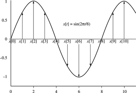
For example, in a CD player, the sampling rate is 44,100 Hz (that is, 44,100 samples per second). Therefore t represents the time in units of a sample period of 1/44,100 Hz = 22.7 microseconds. In this application x[t] represents the signed voltage applied to the loudspeaker at time t.
There are two things to worry about when choosing a representation of x[t]:
1. The dynamic range of the signal—the maximum fluctuation in the signal defined by Equation (8.1). For a signed signal we are interested in the maximum absolute value M possible. For this example, let’s take M = 1 volt.
2. The accuracy required in the representation, sometimes given as a proportion of the maximum range. For example, an accuracy of 100 parts per million means that each x[t] needs to be represented within an error of
Let’s work out the best way of storing x[t] subject to the given dynamic range and accuracy constraints.
We could use a floating-point representation for x[t]. This would certainly meet our dynamic range and accuracy constraints, and it would also be easy to manipulate using the C type float. However, most ARM cores do not support floating point in hardware, and so a floating-point representation would be very slow.
A better choice for fast code is a fixed-point representation. A fixed-point representation uses an integer to represent a fractional value by scaling the fraction. For example, for a maximum error of 0.0001 volts, we only require a step of 0.0002 volts between each representable value. This suggests that we represent x[t] by the integer X[t] defined as
In practice we would rather scale by a power of two. Then we can implement multiplication and division by the scale using shifts. In this case, the smallest power of two greater than 5000 is 213 = 8192. We say that X[t] is a Qk fixed-point representation of x[t] if
In our example we can use a Q13 representation to meet the accuracy required. Since x[t] ranges between −1 and +1 volt, X[t] will range between the integers −8192 and +8192. This range will fit in a 16-bit C variable of type short. Signals that vary between −1 and +1 are often stored as Q15 values because this scales them to the maximum range of a short type integer: −32,768 to +32,767. Note that +1 does not have an exact representation, and we approximate it by +32,767 representing 1 – 2−15. However, we will see in Section 8.1.2 that scaling up to the maximum range is not always a good idea. It increases the probability of overflow when manipulating the fixed-point representations.
In a fixed-point representation we represent each signal value by an integer and use the same scaling for the whole signal. This differs from a floating-point representation, where each signal value x[t] has its own scaling called the exponent dependent upon t.
A common error is to think that floating point is more accurate than fixed point. This is false! For the same number of bits, a fixed-point representation gives greater accuracy. The floating-point representation gives higher dynamic range at the expense of lower absolute accuracy. For example, if you use a 32-bit integer to hold a fixed-point value scaled to full range, then the maximum error in a representation is 2−32. However, single-precision 32-bit floating-point values give a relative error of 2−24. The single-precision floating-point mantissa is 24 bits. The leading 1 of the mantissa is not stored, so 23 bits of storage are actually used. For values near the maximum, the fixed-point representation is 232−24 = 256 times more accurate! The 8-bit floating-point exponent is of little use when you are interested in maximum error rather than relative accuracy.
To summarize, a fixed-point representation is best when there is a clear bound to the strength of the signal and when maximum error is important. When there is no clear bound and you require a large dynamic range, then floating point is better. You can also use the other following representations, which give more dynamic range than fixed point while still being more efficient to implement than floating point.
8.1.1.1 Saturating Fixed-Point Representation
Suppose the maximum value of the signal is not known, but there is a clear range in which the vast majority of samples lie. In this case you can use a fixed-point representation based on the common range. You then saturate or clip any out-of-range samples to the closest available sample in the normal range. This approach gives greater accuracy at the expense of some distortion of very loud signals. See Section 7.7 for hints on efficient saturation.
8.1.1.2 Block-Floating Representation
When small sample values are close to large sample values, they are usually less important. In this case, you can divide the signal into blocks or frames of samples. You can use a different fixed-point scaling on each block or frame according to the strength of the signal in that block or frame.
This is similar to floating point except that we associate a single exponent with a whole frame rather than a single sample. You can use efficient fixed-point operations to operate on the samples within the frame, and you only need costly, exponent-related operations when comparing values among frames.
8.1.1.3 Logarithmic Representation
Suppose your signal x[t] has a large dynamic range. Suppose also that multiplication operations are far more frequent than addition. Then you can use a base-two logarithmic representation. For this representation we consider the related signal y[t]:
Represent y[t] using a fixed-point format. Replace operations of the form
In the second case we arrange that y[c] ≤ y[b]. Calculate the function f (x) = log2(1 + 2x) by using lookup tables and/or interpolation. See Section 7.5 for efficient implementations of log2(x) and 2x.
8.1.2 OPERATING ON VALUES STORED IN FIXED-POINT FORMAT
Suppose now that we have chosen a Qk fixed-point representation for the signal x[t]. In other words, we have an array of integers X[t] such that
Equivalently, if we write the integer X[t] in binary notation, and insert a binary point between bits k and k – 1, then we have the value of x[t]. For example, in Figure 8.2, the fixed-point value 0x6000 at Q15 represents 0.11 in binary, or 3/4 = 0.75 in decimal.
The following subsections cover the basic operations of addition, subtraction, multiplication, division, and square root as applied to fixed-point signals. There are several concepts that apply to all fixed-point operations:
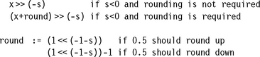
![]() Rounding on right shift. When you perform a right shift to divide by a power of two, the shift rounds towards –∞ rather than rounding to the nearest integer. For a more accurate answer use the operation y = (x + (1
Rounding on right shift. When you perform a right shift to divide by a power of two, the shift rounds towards –∞ rather than rounding to the nearest integer. For a more accurate answer use the operation y = (x + (1 ![]() (shift – 1)))
(shift – 1))) ![]() shift instead. This will round to the nearest integer with 0.5 rounded up. To implement this efficiently, see Section 7.7.3.
shift instead. This will round to the nearest integer with 0.5 rounded up. To implement this efficiently, see Section 7.7.3.
![]() Rounding on divide. For an unsigned divide, calculate y = (x + (d
Rounding on divide. For an unsigned divide, calculate y = (x + (d ![]() 1))/d rather than y = x/d. This gives a rounded result.
1))/d rather than y = x/d. This gives a rounded result.
![]() Headroom. The headroom of a fixed point representation is the ratio of the maximum magnitude that can be stored in the integer to the maximum magnitude that will occur. For example, suppose you use a 16-bit integer to store a Q13 representation of an audio signal that can range between −1 and +1. Then there is a headroom of four times or two bits. You can double a sample value twice without risk of overflowing the 16-bit container integer.
Headroom. The headroom of a fixed point representation is the ratio of the maximum magnitude that can be stored in the integer to the maximum magnitude that will occur. For example, suppose you use a 16-bit integer to store a Q13 representation of an audio signal that can range between −1 and +1. Then there is a headroom of four times or two bits. You can double a sample value twice without risk of overflowing the 16-bit container integer.
![]() Conversion of Q representation. If X[t] is a Qn representation of x[t], then
Conversion of Q representation. If X[t] is a Qn representation of x[t], then
For the following sections we fix signals x[t], c[t], and y[t]. Let X[t], C[t], Y[t] denote their Qn, Qm, Qd fixed-point representations, respectively.
8.1.3 ADDITION AND SUBTRACTION OF FIXED-POINT SIGNALS
The general case is to convert the signal equation
into fixed-point format; that is, approximately:
![]()
Here we use the convention that you should interpret a negative left shift value as a rounded right shift. In other words, we first convert x[t] and c[t] to Qd representations, then add to give Y[t].
We know the values of d, n, and m, at compile time, and so there is no problem in determining the shift direction, or whether there is a shift at all! In practice we usually arrange that n = m = d. Therefore normal integer addition gives a fixed-point addition:
![]()
Provided d = m or d = n, we can perform the operation in a single cycle using the ARM barrel shifter:
![]()
We must be careful though. The preceding equations are only meaningful if the shifted values and the result do not overflow. For example, if Y[t] = X[t] + C[t], then the dynamic range of Y[t] is the sum of the dynamic ranges of X[t] and C[t]. This is liable to overflow the integer container.
There are four common ways you can prevent overflow:
1. Ensure that the X[t] and C[t] representations have one bit of spare headroom each; in other words, each use up only half the range of their integer container. Then there can be no overflow on the addition.
2. Use a larger container type for Y than for X and C. For example, if X[t] and C[t] are stored as 16-bit integers, use a 32-bit integer for Y[t]. This will ensure that there can be no overflow. In fact, Y[t] then has 15 bits of headroom, so you can add many 16-bit values to Y[t] without the possibility of overflow.
3. Use a smaller Q representation for y[t]. For example, if d = n – 1 = m – 1, then the operation becomes
![]()
This operation takes two cycles rather than one since the shift follows the add. However, the operation result cannot overflow.
4. Use saturation. If the value of X[t] + C[t] is outside the range of the integer storing Y[t], then clip it to the nearest possible value that is in range. Section 7.7 shows how to implement saturating arithmetic efficiently.
8.1.4 MULTIPLICATION OF FIXED-POINT SIGNALS
The general case is to convert the signal equation
into fixed point format; that is, approximately:
![]()
You should interpret a negative right shift as a left shift. The product X[t] C[t] is a Q(n + m) representation of Y[t] and the shift converts representation. There are two common uses:
1. We want to accumulate a whole series of products. In this case we set d = n + m, using a wider integer to store Y[t] than X[t] and C[t]. The multiply and multiply accumulate operations are then just
![]()
2. The signal Y[t] is the signal X[t] with pointwise multiplication by some scaling coefficients. In this case, use d = n so that the operation is
![]()
For audio DSP applications, a 16-bit × 16-bit multiply is usually used. Common values for n and m are 14 and 15. As with addition and subtraction it is important to check each operation to make sure that it cannot overflow.
EXAMPLE 8.1
Suppose X[t] is a 16-bit signed representation for an audio signal x[t]. Suppose we need to reduce the power of the signal by a half. To do this we must scale each sample by 1/(![]() ), so c[t] = 2−0.5 = 0.70710678… .
), so c[t] = 2−0.5 = 0.70710678… .
Since we are using a 16-bit representation for X[t], a 16-bit multiply will suffice. The largest power of two that we can multiply c[t] by and have it remain a 16-bit integer is 15. So take n = d, m = 15, and C[t] = 215/(![]() ) = 23,710 = 0x5A82. Therefore we can scale using the integer operation
) = 23,710 = 0x5A82. Therefore we can scale using the integer operation
![]()
8.1.5 DIVISION OF FIXED-POINT SIGNALS
The general case is to convert the signal equation
into fixed point format; that is, approximately:
![]()
Again a negative left shift indicates a right shift. You must take care that the left shift does not cause an overflow. In typical applications, n = m. Then the preceding operation gives a Qd result accurate to d places of binary fraction:
![]()
See Section 7.3.3 for efficient implementations of fixed-point division.
8.1.6 SQUARE ROOT OF A FIXED-POINT SIGNAL
The general case is to convert the signal equation
into fixed point format; that is, approximately:
![]()
The function isqrt finds the nearest integer to the square root of the integer. See Section 7.4 for efficient implementation of square root operations.
8.1.7 SUMMARY: HOW TO REPRESENT A DIGITAL SIGNAL
To choose a representation for a signal value, use the following criteria:
![]() Use a floating-point representation for prototyping algorithms. Do not use floating point in applications where speed is critical. Most ARM implementations do not include hardware floating-point support.
Use a floating-point representation for prototyping algorithms. Do not use floating point in applications where speed is critical. Most ARM implementations do not include hardware floating-point support.
![]() Use a fixed-point representation for DSP applications where speed is critical with moderate dynamic range. The ARM cores provide good support for 8-, 16- and 32-bit fixed-point DSP.
Use a fixed-point representation for DSP applications where speed is critical with moderate dynamic range. The ARM cores provide good support for 8-, 16- and 32-bit fixed-point DSP.
![]() For applications requiring speed and high dynamic range, use a block-floating or logarithmic representation.
For applications requiring speed and high dynamic range, use a block-floating or logarithmic representation.
Table 8.2 summarizes how you can implement standard operations in fixed-point arithmetic. It assumes there are three signals x[t], c[t], y[t], that have Qn, Qm, Qd representations X[t], C[t], Y[t], respectively. In other words:
Table 8.2
Summary of standard fixed-point operations.
| Signal operation | Integer fixed-point equivalent |
| y[t]=x[t] | Y[t]=X[t] <<< (d-n); |
| y[t]=x[t]+c[t] | Y[t]=(X[t] <<< (d-n))+(C[t] <<< (d-m)); |
| y[t]=x[t]-c[t] | Y[t]=(X[t] <<< (d-n))-(C[t] <<< (d-m)); |
| y[t]=x[t]*c[t] | Y[t]=(X[t]*C[t]) <<< (d-n-m); |
| y[t]=x[t]/c[t] | Y[t]=(X[t] <<< (d-n+m))/C[t]; |
| y[t]=sqrt(x[t]) | Y[t]=isqrt(X[t] <<< (2*d-n)); |
To make the table more concise, we use <<< as shorthand for an operation that is either a left or right shift according to the sign of the shift amount. Formally:
![]()
You must always check the precision and dynamic range of the intermediate and output values. Ensure that there are no overflows or unacceptable losses of precision. These considerations determine the representations and size to use for the container integers.
These equations are the most general form. In practice, for addition and subtraction we usually take d = n = m. For multiplication we usually take d = n + m or d = n. Since you know d, n, and m, at compile time, you can eliminate shifts by zero.
8.2 INTRODUCTION TO DSP ON THE ARM
This section begins by looking at the features of the ARM architecture that are useful for writing DSP applications. We look at each common ARM implementation in turn, highlighting its strengths and weaknesses for DSP.
The ARM core is not a dedicated DSP. There is no single instruction that issues a multiply accumulate and data fetch in parallel. However, by reusing loaded data you can achieve a respectable DSP performance. The key idea is to use block algorithms that calculate several results at once, and thus require less memory bandwidth, increase performance, and decrease power consumption compared with calculating single results.
The ARM also differs from a standard DSP when it comes to precision and saturation. In general, ARM does not provide operations that saturate automatically. Saturating versions of operations usually cost additional cycles. Section 7.7 covered saturating operations on the ARM. On the other hand, ARM supports extended-precision 32-bit multiplied by 32-bit to 64-bit operations very well. These operations are particularly important for CD-quality audio applications, which require intermediate precision at greater than 16 bits.
From ARM9 onwards, ARM implementations use a multistage execute pipeline for loads and multiplies, which introduces potential processor interlocks. If you load a value and then use it in either of the following two instructions, the processor may stall for a number of cycles waiting for the loaded value to arrive. Similarly if you use the result of a multiply in the following instruction, this may cause stall cycles. It is particularly important to schedule code to avoid these stalls. See the discussion in Section 6.3 on instruction scheduling.
SUMMARY: Guidelines for Writing DSP Code for ARM
![]() Design the DSP algorithm so that saturation is not required because saturation will cost extra cycles. Use extended-precision arithmetic or additional scaling rather than saturation.
Design the DSP algorithm so that saturation is not required because saturation will cost extra cycles. Use extended-precision arithmetic or additional scaling rather than saturation.
![]() Design the DSP algorithm to minimize loads and stores. Once you load a data item, then perform as many operations that use the datum as possible. You can often do this by calculating several output results at once. Another way of increasing reuse is to concatenate several operations. For example, you could perform a dot product and signal scale at the same time, while only loading the data once.
Design the DSP algorithm to minimize loads and stores. Once you load a data item, then perform as many operations that use the datum as possible. You can often do this by calculating several output results at once. Another way of increasing reuse is to concatenate several operations. For example, you could perform a dot product and signal scale at the same time, while only loading the data once.
![]() Write ARM assembly to avoid processor interlocks. The results of load and multiply instructions are often not available to the next instruction without adding stall cycles. Sometimes the results will not be available for several cycles. Refer to Appendix D for details of instruction cycle timings.
Write ARM assembly to avoid processor interlocks. The results of load and multiply instructions are often not available to the next instruction without adding stall cycles. Sometimes the results will not be available for several cycles. Refer to Appendix D for details of instruction cycle timings.
![]() There are 14 registers available for general use on the ARM, r0 to r12 and r14. Design the DSP algorithm so that the inner loop will require 14 registers or fewer.
There are 14 registers available for general use on the ARM, r0 to r12 and r14. Design the DSP algorithm so that the inner loop will require 14 registers or fewer.
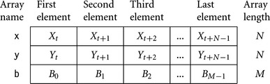
In the following sections we look at each of the standard ARM cores in turn. We implement a dot-product example for each core. A dot-product is one of the simplest DSP operations and highlights the difference among different ARM implementations. A dot-product combines N samples from two signals xt and ct to produce a correlation value a:

The C interface to the dot-product function is where
![]()
![]() sample is the type to hold a 16-bit audio sample, usually a short
sample is the type to hold a 16-bit audio sample, usually a short
![]() coefficient is the type to hold a 16-bit coefficient, usually a short
coefficient is the type to hold a 16-bit coefficient, usually a short
![]() x[i] and c[i] are two arrays of length N (the data and coefficients)
x[i] and c[i] are two arrays of length N (the data and coefficients)
![]() the function returns the accumulated 32-bit integer dot product a
the function returns the accumulated 32-bit integer dot product a
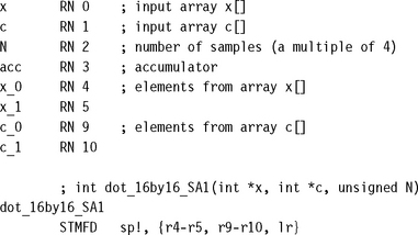
8.2.1 DSP ON THE ARM7TDMI
The ARM7TDMI has a 32-bit by 8-bit per cycle multiply array with early termination. It takes four cycles for a 16-bit by 16-bit to 32-bit multiply accumulate. Load instructions take three cycles and store instructions two cycles for zero-wait-state memory or cache. See Section D.2 in Appendix D for details of cycle timings for ARM7TDMI instructions.
SUMMARY: Guidelines for Writing DSP Code for the ARM7TDMI
![]() Load instructions are slow, taking three cycles to load a single value. To access memory efficiently use load and store multiple instructions LDM and STM. Load and store multiples only require a single cycle for each additional word transferred after the first word. This often means it is more efficient to store 16-bit data values in 32-bit words.
Load instructions are slow, taking three cycles to load a single value. To access memory efficiently use load and store multiple instructions LDM and STM. Load and store multiples only require a single cycle for each additional word transferred after the first word. This often means it is more efficient to store 16-bit data values in 32-bit words.
![]() The multiply instructions use early termination based on the second operand in the product Rs. For predictable performance use the second operand to specify constant coefficients or multiples.
The multiply instructions use early termination based on the second operand in the product Rs. For predictable performance use the second operand to specify constant coefficients or multiples.
![]() Multiply is one cycle faster than multiply accumulate. It is sometimes useful to split an MLA instruction into separate MUL and ADD instructions. You can then use a barrel shift with the ADD to perform a scaled accumulate.
Multiply is one cycle faster than multiply accumulate. It is sometimes useful to split an MLA instruction into separate MUL and ADD instructions. You can then use a barrel shift with the ADD to perform a scaled accumulate.
![]() You can often multiply by fixed coefficients faster using arithmetic instructions with shifts. For example, 240x = (x
You can often multiply by fixed coefficients faster using arithmetic instructions with shifts. For example, 240x = (x ![]() 8) – (x
8) – (x ![]() 4). For any fixed coefficient of the form ±2a ± 2b ± 2c, ADD and SUB with shift give a faster multiply accumulate than MLA.
4). For any fixed coefficient of the form ±2a ± 2b ± 2c, ADD and SUB with shift give a faster multiply accumulate than MLA.
EXAMPLE 8.2
This example shows a 16-bit dot-product optimized for the ARM7TDMI. Each MLA takes a worst case of four cycles. We store the 16-bit input samples in 32-bit words so that we can use the LDM instruction to load them efficiently.
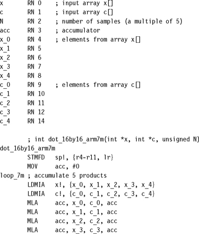
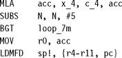
This code assumes that the number of samples N is a multiple of five. Therefore we can use a five-word load multiple to increase data bandwidth. The cost per load is 7/4 = 1.4 cycles compared to 3 cycles per load if we had used LDR or LDRSH. The inner loop requires a worst case of 7 + 7 + 5 * 4 + 1 + 3 = 38 cycles to process each block of 5 products from the sum. This gives the ARM7TDMI a DSP rating of 38/5 = 7.6 cycles per tap for a 16-bit dot-product. The block filter algorithm of Section 8.3 gives a much better performance per tap if you are calculating multiple products.
8.2.2 DSP ON THE ARM9TDMI
The ARM9TDMI has the same 32-bit by 8-bit per cycle multiplier array with early termination as the ARM7TDMI. However, load and store operations are much faster compared to the ARM7TDMI. They take one cycle provided that you do not attempt to use the loaded value for two cycles after the load instruction. See Section D.3 in Appendix D for cycle timings of ARM9TDMI instructions.
SUMMARY: Writing DSP Code for the ARM9TDMI
![]() Load instructions are fast as long as you schedule the code to avoid using the loaded value for two cycles. There is no advantage to using load multiples. Therefore you should store 16-bit data in 16-bit short type arrays. Use the LDRSH instruction to load the data.
Load instructions are fast as long as you schedule the code to avoid using the loaded value for two cycles. There is no advantage to using load multiples. Therefore you should store 16-bit data in 16-bit short type arrays. Use the LDRSH instruction to load the data.
![]() The multiply instructions use early termination based on the second operand in the product Rs. For predictable performance use the second operand to specify constant coefficients or multiples.
The multiply instructions use early termination based on the second operand in the product Rs. For predictable performance use the second operand to specify constant coefficients or multiples.
![]() Multiply is the same speed as multiply accumulate. Try to use the MLA instruction rather than a separate multiply and add.
Multiply is the same speed as multiply accumulate. Try to use the MLA instruction rather than a separate multiply and add.
![]() You can often multiply by fixed coefficients faster using arithmetic instructions with shifts. For example, 240x = (x
You can often multiply by fixed coefficients faster using arithmetic instructions with shifts. For example, 240x = (x ![]() 8) – (x
8) – (x ![]() 4). For any fixed coefficient of the form ±2a ± 2b ± 2c, ADD and SUB with shift give a faster multiply accumulate than using MLA.
4). For any fixed coefficient of the form ±2a ± 2b ± 2c, ADD and SUB with shift give a faster multiply accumulate than using MLA.
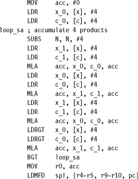
EXAMPLE 8.3
This example shows a 16-bit dot-product optimized for the ARM9TDMI. Each MLA takes a worst case of four cycles. We store the 16-bit input samples in 16-bit short integers, since there is no advantage in using LDM rather than LDRSH, and using LDRSH reduces the memory size of the data.

We have assumed that the number of samples N is a multiple of four. Therefore we can unroll the loop four times to increase performance. The code is scheduled so that there are four instructions between a load and the use of the loaded value. This uses the preload tricks of Section 6.3.1.1:
![]() The loads are double buffered. We use x0, c0 while we are loading x1, c1 and vice versa.
The loads are double buffered. We use x0, c0 while we are loading x1, c1 and vice versa.
![]() We load the initial values x0, c0, before the inner loop starts. This initiates the double buffer process.
We load the initial values x0, c0, before the inner loop starts. This initiates the double buffer process.
![]() We are always loading one pair of values ahead of the ones we are using. Therefore we must avoid the last pair of loads or we will read off the end of the arrays. We do this by having a loop counter that counts down to zero on the last loop. Then we can make the final loads conditional on N > 0.
We are always loading one pair of values ahead of the ones we are using. Therefore we must avoid the last pair of loads or we will read off the end of the arrays. We do this by having a loop counter that counts down to zero on the last loop. Then we can make the final loads conditional on N > 0.
The inner loop requires 28 cycles per loop, giving 28/4 = 7 cycles per tap. See Section 8.3 for more efficient block filter implementations.
8.2.3 DSP ON THE STRONGARM
The StrongARM core SA-1 has a 32-bit by 12-bit per cycle signed multiply array with early termination. If you attempt to use a multiply result in the following instruction, or start a new multiply, then the core will stall for one cycle. Load instructions take one cycle, except for signed byte and halfword loads, which take two cycles. There is a one-cycle delay before you can use the loaded value. See Section D.4 in Appendix D for details of the StrongARM instruction cycle timings.
SUMMARY: Writing DSP Code for the StrongARM
![]() Avoid signed byte and halfword loads. Schedule the code to avoid using the loaded value for one cycle. There is no advantage to using load multiples.
Avoid signed byte and halfword loads. Schedule the code to avoid using the loaded value for one cycle. There is no advantage to using load multiples.
![]() The multiply instructions use early termination based on the second operand in the product Rs. For predictable performance use the second operand to specify constant coefficients or multiples.
The multiply instructions use early termination based on the second operand in the product Rs. For predictable performance use the second operand to specify constant coefficients or multiples.
![]() Multiply is the same speed as multiply accumulate. Try to use the MLA instruction rather than a separate multiply and add.
Multiply is the same speed as multiply accumulate. Try to use the MLA instruction rather than a separate multiply and add.
EXAMPLE 8.4
This example shows a 16-bit dot-product. Since a signed 16-bit load requires two cycles, it is more efficient to use 32-bit data containers for the StrongARM. To schedule StrongARM code, one trick is to interleave loads and multiplies.
We have assumed that the number of samples N is a multiple of four and so have unrolled by four times. For worst-case 16-bit coefficients, each multiply requires two cycles. We have scheduled to remove all load and multiply use interlocks. The inner loop uses 19 cycles to process 4 taps, giving a rating of 19/4 = 4.75 cycles per tap.
8.2.4 DSP ON THE ARM9E
The ARM9E core has a very fast pipelined multiplier array that performs a 32-bit by 16-bit multiply in a single issue cycle. The result is not available on the next cycle unless you use the result as the accumulator in a multiply accumulate operation. The load and store operations are the same speed as on the ARM9TDMI. See Section D.5 in Appendix D for details of the ARM9E instruction cycle times.
To access the fast multiplier, you will need to use the multiply instructions defined in the ARMv5TE architecture extensions. For 16-bit by 16-bit products use SMULxy and SMLAxy. See Appendix A for a full list of ARM multiply instructions.
SUMMARY: Writing DSP Code for the ARM9E
![]() The ARMv5TE architecture multiply operations are capable of unpacking 16-bit halves from 32-bit words and multiplying them. For best load bandwidth you should use word load instructions to load packed 16-bit data items. As for the ARM9TDMI you should schedule code to avoid load use interlocks.
The ARMv5TE architecture multiply operations are capable of unpacking 16-bit halves from 32-bit words and multiplying them. For best load bandwidth you should use word load instructions to load packed 16-bit data items. As for the ARM9TDMI you should schedule code to avoid load use interlocks.
![]() The multiply operations do not early terminate. Therefore you should only use MUL and MLA for multiplying 32-bit integers. For 16-bit values use SMULxy and SMLAxy.
The multiply operations do not early terminate. Therefore you should only use MUL and MLA for multiplying 32-bit integers. For 16-bit values use SMULxy and SMLAxy.
![]() Multiply is the same speed as multiply accumulate. Try to use the SMLAxy instruction rather than a separate multiply and add.
Multiply is the same speed as multiply accumulate. Try to use the SMLAxy instruction rather than a separate multiply and add.
EXAMPLE 8.5
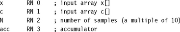
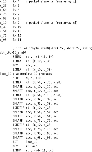
This example shows the dot-product for the ARM9E. It assumes that the ARM is configured for a little-endian memory system. If the ARM is configured for a big-endian memory system, then you need to swap the B and T instruction suffixes. You can use macros to do this for you automatically as in Example 8.11. We use the naming convention x_10 to mean that the top 16 bits of the register holds x1 and the bottom 16 bits x0.
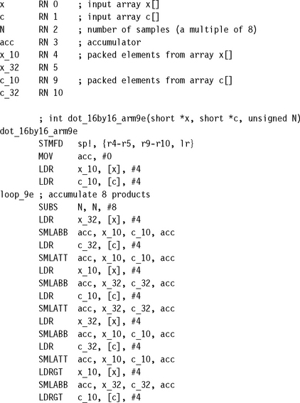
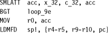
We have unrolled eight times, assuming that N is a multiple of eight. Each load instruction reads two 16-bit values, giving a high memory bandwidth. The inner loop requires 20 cycles to accumulate 8 products, a rating of 20/8 = 2.5 cycles per tap. A block filter gives even greater efficiency.
8.2.5 DSP ON THE ARM10E
Like ARM9E, the ARM10E core also implements ARM architecture ARMv5TE. The range and speed of multiply operations is the same as for the ARM9E, except that the 16-bit multiply accumulate requires two cycles rather than one. For details of the ARM10E core cycle timings, see Section D.6 in Appendix D.
The ARM10E implements a background loading mechanism to accelerate load and store multiples. A load or store multiple instruction issues in one cycle. The operation will run in the background, and if you attempt to use the value before the background load completes, then the core will stall. ARM10E uses a 64-bit-wide data path that can transfer two registers on every background cycle. If the address isn’t 64-bit aligned, then only 32 bits can be transferred on the first cycle.
SUMMARY: Writing DSP Code for the ARM10E
![]() Load and store multiples run in the background to give a high memory bandwidth. Use load and store multiples whenever possible. Be careful to schedule the code so that it does not use data before the background load has completed.
Load and store multiples run in the background to give a high memory bandwidth. Use load and store multiples whenever possible. Be careful to schedule the code so that it does not use data before the background load has completed.
![]() Ensure data arrays are 64-bit aligned so that load and store multiple operations can transfer two words per cycle.
Ensure data arrays are 64-bit aligned so that load and store multiple operations can transfer two words per cycle.
![]() The multiply operations do not early terminate. Therefore you should only use MUL and MLA for multiplying 32-bit integers. For 16-bit values use SMULxy and SMLAxy.
The multiply operations do not early terminate. Therefore you should only use MUL and MLA for multiplying 32-bit integers. For 16-bit values use SMULxy and SMLAxy.
![]() The SMLAxy instruction takes one cycle more than SMULxy. It may be useful to split a multiply accumulate into a separate multiply and add.
The SMLAxy instruction takes one cycle more than SMULxy. It may be useful to split a multiply accumulate into a separate multiply and add.
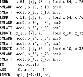
8.2.6 DSP ON THE INTEL XSCALE
The Intel XScale implements version ARMv5TE of the ARM architecture like ARM9E and ARM10E. The timings of load and multiply instructions are similar to the ARM9E, and code you’ve optimized for the ARM9E should run efficiently on XScale. See Section D.7 in Appendix D for details of the XScale core cycle timings.
SUMMARY: Writing DSP Code for the Intel XScale
![]() The load double word instruction LDRD can transfer two words in a single cycle. Schedule the code so that you do not use the first loaded register for two cycles and the second for three cycles.
The load double word instruction LDRD can transfer two words in a single cycle. Schedule the code so that you do not use the first loaded register for two cycles and the second for three cycles.
![]() Ensure data arrays are 64-bit aligned so that you can use the 64-bit load instruction LDRD.
Ensure data arrays are 64-bit aligned so that you can use the 64-bit load instruction LDRD.
![]() The result of a multiply is not available immediately. Following a multiply with another multiply may introduce stalls. Schedule code so that multiply instructions are interleaved with load instructions to prevent processor stalls.
The result of a multiply is not available immediately. Following a multiply with another multiply may introduce stalls. Schedule code so that multiply instructions are interleaved with load instructions to prevent processor stalls.
![]() The multiply operations do not early terminate. Therefore you should only use MUL and MLA for multiplying 32-bit integers. For 16-bit values use SMULxy and SMLAxy.
The multiply operations do not early terminate. Therefore you should only use MUL and MLA for multiplying 32-bit integers. For 16-bit values use SMULxy and SMLAxy.

8.3 FIR FILTERS
The finite impulse response (FIR) filter is a basic building block of many DSP applications and worth investigating in some detail. You can use a FIR filter to remove unwanted frequency ranges, boost certain frequencies, or implement special effects. We will concentrate on efficient implementation of the filter on the ARM. The FIR filter is the simplest type of digital filter. The filtered sample yt depends linearly on a fixed, finite number of unfiltered samples xt. Let M be the length of the filter. Then for some filter coefficients, ci:
Some books refer to the coefficients ci as the impulse response. If you feed the impulse signal x = (1, 0, 0, 0, …) into the filter, then the output is the signal of filter coefficients y = (c0, c1, c2, …).
Let’s look at the issue of dynamic range and possible overflow of the output signal. Suppose that we are using Qn and Qm fixed-point representations X[t] and C[i] for xt and ci, respectively. In other words:
We implement the filter by calculating accumulated values A[t]:
Then A[t] is a Q(n+m) representation of yt. But, how large is A[t]? How many bits of precision do we need to ensure that A[t] does not overflow its integer container and give a meaningless filter result? There are two very useful inequalities that answer these questions:
Equation (8.24) says that if you know the dynamic range of X[t], then the maximum gain of dynamic range is bounded by the sum of the absolute values of the filter coefficients C[i]. Equation (8.25) says that if you know the power of the signal X[t], then the dynamic range of A[t] is bounded by the product of the input signal and coefficient powers. Both inequalities are the best possible. Given fixed C[t], we can choose X[t] so that there is equality. They are special cases of the more general Holder inequalities. Let’s illustrate with an example.
EXAMPLE 8.8
Consider the simple, crude, high-pass filter defined by Equation (8.26). The filter allows through high-frequency signals, but attenuates low-frequency ones.
Suppose we represent xi and ci by Qn, Qm 16-bit fixed-point signals X[t] and C[i]. Then,
Since X[t] is a 16-bit integer, |X[t]| ≤ 215, and so, using the first inequality above,
A[t] will not overflow a 32-bit integer, provided that m ≤ 15. So, take m = 15 for greatest coefficient accuracy. The following integer calculation implements the filter with 16-bit Qn input X[t] and 32-bit Q(n + 15) output A[t]:
![]()
For a Qn output Y[t] we need to set Y[t]= A[t] ![]() 15. However, this could overflow a 16-bit integer. Therefore you either need to saturate the result, or store the result using a Q(n – 1) representation.
15. However, this could overflow a 16-bit integer. Therefore you either need to saturate the result, or store the result using a Q(n – 1) representation.
8.3.1 BLOCK FIR FILTERS
Example 8.8 shows that we can usually implement filters using integer sums of products, without the need to check for saturation or overflow:
![]()
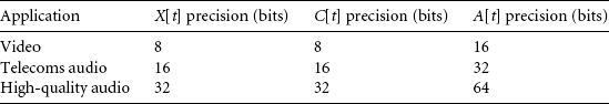
Generally X[t] and C[i] are k-bit integers and A[t] is a 2k-bit integer, where k = 8, 16, or 32. Table 8.3 shows the precision for some typical applications.
We will look at detailed examples of long 16-bit and 32-bit filters. By a long filter, we mean that M is so large that you can’t hold the filter coefficients in registers. You should optimize short filters such as Example 8.8 on a case-by-case basis. For these you can hold many coefficients in registers.
For a long filter, each result A[t] depends on M data values and M coefficients that we must read from memory. These loads are time consuming, and it is inefficient to calculate just a single result A[t]. While we are loading the data and coefficients, we can calculate A[t + 1] and possibly A[t + 2] at the same time.
An R-way block filter implementation calculates the R values A[t], A[t + 1], …, A[t + R – 1] using a single pass of the data X[t] and coefficients C[i]. This reduces the number of memory accesses by a factor of R over calculating each result separately. So R should be as large as possible. On the other hand, the larger R is, the more registers we require to hold accumulated values and data or coefficients. In practice we choose R to be the largest value such that we do not run out of registers in the inner loop. On ARM R can range from 2 to 6, as we will show in the following code examples.
An R × S block filter is an R-way block filter where we read S data and coefficient values at a time for each iteration of the inner loop. On each loop we accumulate R × S products onto the R accumulators.
Figure 8.3 shows a typical 4 × 3 block filter implementation. Each accumulator on the left is the sum of products of the coefficients on the right multiplied by the signal value heading each column. The diagram starts with the oldest sample Xt–M+1 since the filter routine will load samples in increasing order of memory address. Each inner loop of a4 × 3 filter accumulates the 12 products in a 4 × 3 parallelogram. We’ve shaded the first parallelogram and the first sample of the third parallelogram.
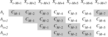
As you can see from Figure 8.3, an R × S block filter implementation requires R accumulator registers and a history of R – 1 input samples. You also need a register to hold the next coefficient. The loop repeats after adding S products to each accumulator. Therefore we must allocate X[t] and X[t – S] to the same register. We must also keep the history of length at least R – 1 samples in registers. Therefore S ≥ R – 1. For this reason, block filters are usually of size R × (R – 1) or R × R.
The following examples give optimized block FIR implementations. We select the best values for R and S for different ARM implementations. Note that for these implementations, we store the coefficients in reverse order in memory. Figure 8.3 shows that we start from coefficient C[M – 1] and work backwards.
EXAMPLE 8.9
As with the ARM7TDMI dot product, we store 16-bit and 32-bit data items in 32- bit words. Then we can use load multiples for maximum load efficiency. This example implements a 4 × 3 block filter for 16-bit input data. The array pointers a, x, and c point to output and input arrays of the formats given in Figure 8.4.
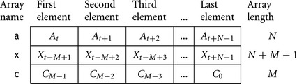
Note that the x array holds a history of M – 1 samples and that we reverse the coefficient array. We hold the coefficient array pointer c and length M in a structure, which limits the function to four register arguments. We also assume that N is a multiple of four and M a multiple of three.
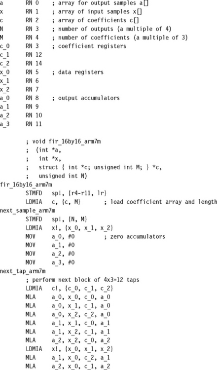

Each iteration of the inner loop processes the next three coefficients and updates four filter outputs. Assuming the coefficients are 16-bit, each multiply accumulate requires 4 cycles. Therefore it processes 12 filter taps in 62 cycles, giving a block FIR rating of 5.17 cycles/tap.
Note that it is cheaper to reset the coefficient and input pointers c and x using a subtraction, rather than save their values on the stack.
EXAMPLE 8.10
This example gives an optimized block filter for the ARM9TDMI. First, the ARM9TDMI has a single-cycle 16-bit load, so there is no advantage in using load multiples. We can save memory by storing the data and coefficients in 16-bit halfwords. Second, we can use a 4 × 4 block filter implementation rather than a 4 × 3 implementation. This reduces the loop overhead and is useful if the number of coefficients is a multiple of four rather than a multiple of three.
The input and output arrays have the same format as Example 8.9, except that the input arrays are now 16-bit. The number of outputs and coefficients, N and M, must be multiples of four.
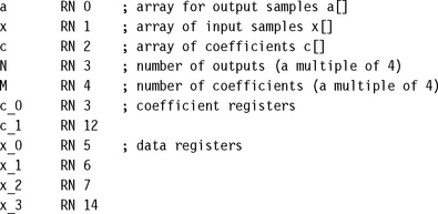
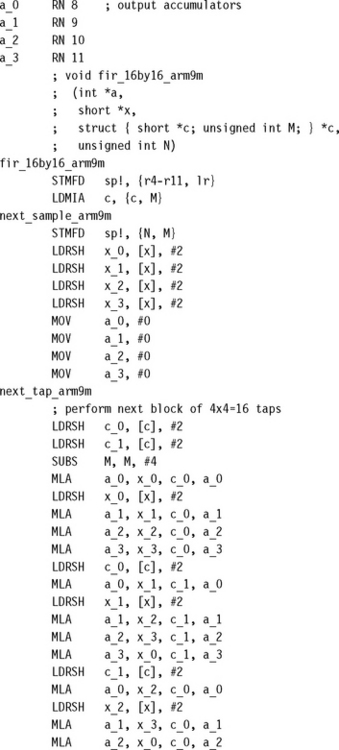
The code is scheduled so that we don’t use a loaded value on the following two cycles. We’ve moved the loop counter decrement to the start of the loop to fill a load delay slot.
Each iteration of the inner loop processes the next four coefficients and updates four filter outputs. Assuming the coefficients are 16 bits, each multiply accumulate requires 4 cycles. Therefore it processes 16 filter taps in 76 cycles, giving a block FIR rating of 4.75 cycles/tap.
This code also works well for other ARMv4 architecture processors such as the StrongARM. On StrongARM the inner loop requires 61 cycles, or 3.81 cycles/tap.
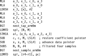
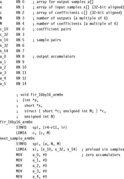
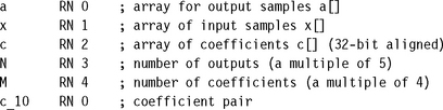
EXAMPLE 8.11
The ARM9E has a faster multiplier than previous ARM processors. The ARMv5TE 16-bit multiply instructions also unpack 16-bit data when two 16-bit values are packed into a single 32-bit word. Therefore we can store more data and coefficients in registers and use fewer load instructions.
This example implements a 6 × 6 block filter for ARMv5TE processors. The routine is rather long because it is optimized for maximum speed. If you don’t require as much performance, you can reduce code size by using a 4 × 4 block implementation.
The input and output arrays have the same format as Example 8.9, except that the input arrays are now 16-bit values. The number of outputs and coefficients, N and M, must be multiples of six. The input arrays must be 32-bit aligned and the memory system little-endian. If you need to write endian-neutral routines, then you should replace SMLAxy instructions by macros that change the T and B settings according to endianness. For example the following macro, SMLA00, evaluates to SMLABB or SMLATT for little- or big-endian memory systems, respectively. If b and c are read as arrays of 16-bit values, then SMLA00 always multiplies b[0] by c[0] regardless of endianness.
![]()
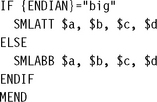
To keep the example simple, we haven’t used macros like this. The following code only works on a little-endian memory system.

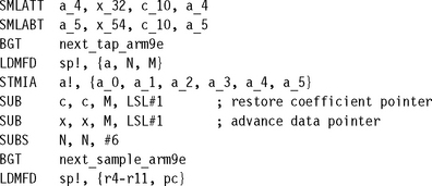
Each iteration of the inner loop updates the next six filter outputs, accumulating six products to each output. Table 8.4 shows the cycle timings for ARMv5TE architecture processors.
EXAMPLE 8.12
Sometimes 16-bit data items do not give a large enough dynamic range. The ARMv5TE architecture adds an instruction SMLAWx that allows for efficient filtering of 32-bit data by 16-bit coefficients. The instruction multiplies a 32-bit data item by a 16-bit coefficient, extracts the top 32 bits of the 48-bit result, and adds it to a 32-bit accumulator.
This example implements a 5 × 4 block FIR filter with 32-bit data and 16-bit coefficients. The input and output arrays have the same format as Example 8.9, except that the coefficient array is 16-bit. The number of outputs must be a multiple of five and the number of coefficients a multiple of four. The input coefficient array must be 32-bit aligned and the memory system little-endian. As described in Example 8.11, you can write endian-neutral code by using macros.
If the input samples and coefficients use Qn and Qm representations, respectively, then the output is Q(n + m – 16). The SMLAWx shifts down by 16 to prevent overflow.
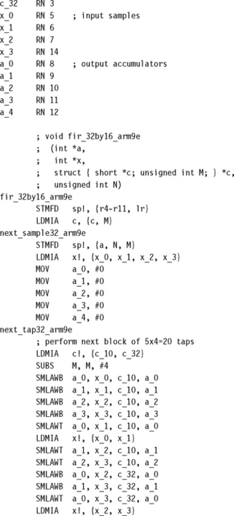
Each iteration of the inner loop updates five filter outputs, accumulating four products to each. Table 8.5 gives cycle counts for architecture ARMv5TE processors.
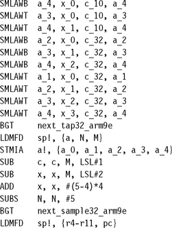
EXAMPLE 8.13
High-quality audio applications often require intermediate sample precision at greater than 16-bit. On the ARM we can use the long multiply instruction SMLAL to implement an efficient filter with 32-bit input data and coefficients. The output values are 64-bit. This makes the ARM very competitive for CD audio quality applications.
The output and input arrays have the same format as in Example 8.9. We implement a3 × 2 block filter so N must be a multiple of three and M a multiple of two. The filter works well on any ARMv4 implementation.
![]()
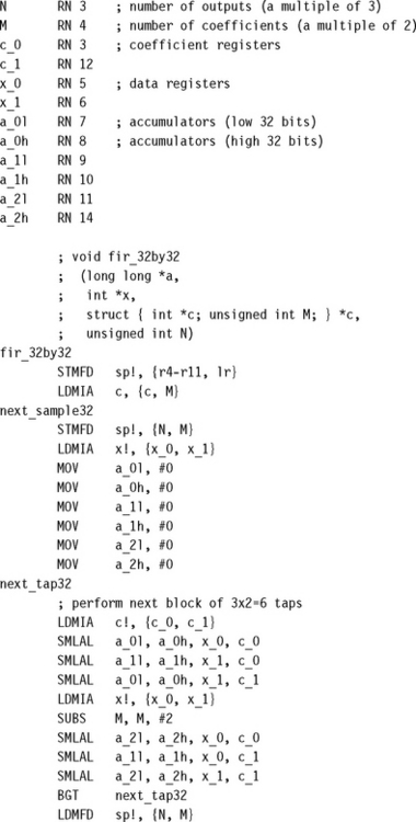
Each iteration of the inner loop processes the next two coefficients and updates three filter outputs. Assuming the coefficients use the full 32-bit range, the multiply does not terminate early. The routine is optimal for most ARM implementations. Table 8.6 gives the cycle timings for a range of processors.
SUMMARY: Writing FIR Filters on the ARM
![]() If the number of FIR coefficients is small enough, then hold the coefficients and history samples in registers. Often coefficients are repeated. This will save on the number of registers you need.
If the number of FIR coefficients is small enough, then hold the coefficients and history samples in registers. Often coefficients are repeated. This will save on the number of registers you need.
![]() If the FIR filter length is long, then use a block filter algorithm of size R × (R – 1) or R × R. Choose the largest R possible given the 14 available general purpose registers on the ARM.
If the FIR filter length is long, then use a block filter algorithm of size R × (R – 1) or R × R. Choose the largest R possible given the 14 available general purpose registers on the ARM.
![]() Ensure that the input arrays are aligned to the access size. This will be 64-bit when using LDRD. Ensure that the array length is a multiple of the block size.
Ensure that the input arrays are aligned to the access size. This will be 64-bit when using LDRD. Ensure that the array length is a multiple of the block size.
8.4 IIR FILTERS
An infinite impulse response (IIR) filter is a digital filter that depends linearly on a finite number of input samples and a finite number of previous filter outputs. In other words, it combines a FIR filter with feedback from previous filter outputs. Mathematically, for some coefficients bi and aj:
If you feed in the impulse signal x = (1, 0, 0, 0, …), then yt may oscillate forever. This is why it has an infinite impulse response. However, for a stable filter, yt will decay to zero. We will concentrate on efficient implementation of this filter.
You can calculate the output signal yt directly, using Equation (8.29). In this case the code is similar to the FIR of Section 8.3. However, this calculation method may be numerically unstable. It is often more accurate, and more efficient, to factorize the filter into a series of biquads—an IIR filter with M = L = 2:
We can implement any IIR filter by repeatedly filtering the data by a number of biquads. To see this, we use the z-transform. This transform associates with each signal xt, a polynomial x(z) defined as
If we transform the IIR equation into z-coordinates, we obtain
Next, consider H(z) as the ratio of two polynomials in z−1. We can factorize the polynomials into quadratic factors. Then we can express H(z) as a product of quadratic ratios Hi(z), each Hi(z) representing a biquad.
So, now we only have to implement biquads efficiently. On the face of it, to calculate yt for a biquad, we need the current sample xt and four history elements xt−1, xt−2, yt−1, yt−2. However, there is a trick to reduce the number of history or state values we require from four to two. We define an intermediate signal st by
In other words, we perform the feedback part of the filter before the FIR part of the filter. Equivalently we apply the denominator of H(z) before the numerator. Now each biquad filter requires a state of only two values, st−1 and st−2.
The coefficient b0 controls the amplitude of the biquad. We can assume that b0 = 1 when performing a series of biquads, and use a single multiply or shift at the end to correct the signal amplitude. So, to summarize, we have reduced an IIR to filtering by a series of biquads of the form
To implement each biquad, we need to store fixed-point representations of the six values –a1, –a2, b1, b2, st−1, st−2 in ARM registers. To load a new biquad requires six loads; to load a new sample, only one load. Therefore it is much more efficient for the inner loop to loop over samples rather than loop over biquads.
For a block IIR, we split the input signal xt into large frames of N samples. We make multiple passes over the signal, filtering by as many biquads as we can hold in registers on each pass. Typically for ARMv4 processors we filter by one biquad on each pass; for ARMv5TE processors, by two biquads. The following examples give IIR code for different ARM processors.
EXAMPLE 8.14
This example implements a 1 × 2 block IIR filter on the ARM7TDMI. Each inner loop applies one biquad filter to the next two input samples. The input arrays have the format given in Figure 8.5.
Each biquad Bk is a list of six values (–a1, –a2, b1, b2, st−1, st−2). As with previous implementations for the ARM7TDMI, we store the 16-bit input values in 32-bit integers so we can use load multiples. We store the biquad coefficients at Q14 fixed-point format. The number of samples N must be even.
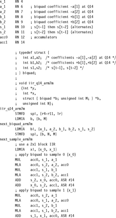

Each inner loop requires a worst case of 44 cycles to apply one biquad to two samples. This gives the ARM7TDMI an IIR rating of 22 cycles/biquad-sample for a general biquad.
EXAMPLE 8.15
On the ARM9TDMI we can use halfword load instructions rather than load multiples. Therefore we can store samples in 16-bit short integers. This example implements a load scheduled IIR suitable for the ARM9TDMI. The interface is the same as in Example 8.14, except that we use 16-bit data items.
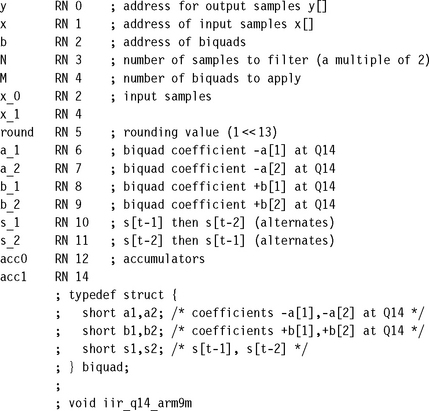

The timings on ARM9TDMI and StrongARM are shown in Table 8.7.
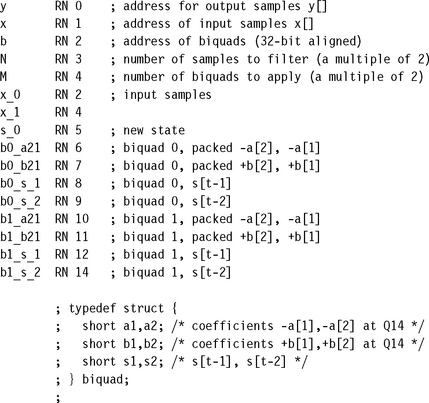
EXAMPLE 8.16
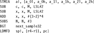
With ARMv5TE processors, we can pack two 16-bit values into each register. This means we can store the state and coefficients for two biquads in registers at the same time. This example implements a 2 × 2 block IIR filter. Each iteration of the inner loop applies two biquad filters to the next two input samples.
The format of the input arrays is the same as for Example 8.14, except that we use 16-bit arrays. The biquad array must be 32-bit aligned. The number of samples N and number of biquads M must be even.
As with the ARM9E FIR, the routine only works for a little-endian memory system. See the discussion in Example 8.11 on how to write endian-neutral DSP code using macros.
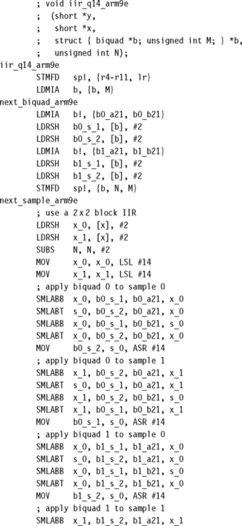
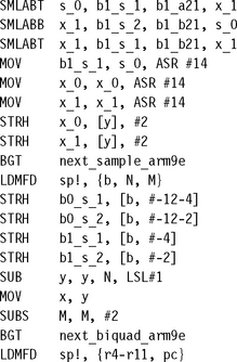
The timings on ARM9E, ARM10E, and XScale are shown in Table 8.8.
SUMMARY: Implementing 16-bit IIR Filters
![]() Factorize the IIR into a series of biquads. Choose the data precision so there can be no overflow during the IIR calculation. To compute the maximum gain of an IIR, apply the IIR to an impulse to generate the impulse response. Apply the equations of Section 8.3 to the impulse response c[j].
Factorize the IIR into a series of biquads. Choose the data precision so there can be no overflow during the IIR calculation. To compute the maximum gain of an IIR, apply the IIR to an impulse to generate the impulse response. Apply the equations of Section 8.3 to the impulse response c[j].
![]() Use a block IIR algorithm, dividing the signal to be filtered into large frames.
Use a block IIR algorithm, dividing the signal to be filtered into large frames.
![]() On each pass of the sample frame, filter by M biquads. Choose M to be the largest number of biquads so that you can hold the state and coefficients in the 14 available registers on the ARM. Ensure that the total number of biquads is a multiple of M.
On each pass of the sample frame, filter by M biquads. Choose M to be the largest number of biquads so that you can hold the state and coefficients in the 14 available registers on the ARM. Ensure that the total number of biquads is a multiple of M.
![]() As always, schedule code to avoid load and multiply use interlocks.
As always, schedule code to avoid load and multiply use interlocks.
8.5 THE DISCRETE FOURIER TRANSFORM
The Discrete Fourier Transform (DFT) converts a time domain signal xt to a frequency domain signal yk. The associated inverse transform (IDFT) reconstructs the time domain signal from the frequency domain signal. This tool is heavily used in signal analysis and compression. It is particularly powerful because there is an algorithm, the Fast Fourier Transform (FFT), that implements the DFT very efficiently. In this section we will look at some efficient ARM implementations of the FFT.
The DFT acts on a frame of N complex time samples, converting them into N complex frequency coefficients. We will use Equations (8.37) and (8.38) as the definition. You may see slightly different equations in different texts because some authors may use a different scaling or a different definition of which is the forward and which the inverse transform. This doesn’t affect any of the important properties of the transform.
As you can see, the transforms are the same except for scaling and choice of wN. Therefore we’ll only look at the forward transform. In fact the Fast Fourier Transform algorithm works for any wN such that ![]() . The algorithm is only invertible for principal roots of unity where
. The algorithm is only invertible for principal roots of unity where ![]() for k < N.
for k < N.
8.5.1 THE FAST FOURIER TRANSFORM
The idea of the FFT is to break down the transform by factorizing N. Suppose for example that N = R × S. Split the output into S blocks of size R and the input into R blocks of size S. In other words:
Equation (8.42) reduces the N-point DFT to S sets of R-point DFTs, N multiplications by coefficients of the form ![]() , and R sets of S-point DFTs. Specifically, if we set in turn:
, and R sets of S-point DFTs. Specifically, if we set in turn:
In practice we then repeat this process to calculate the R- and S-point DFTs efficiently. This works well when N has many small factors. The most useful case is when N is a power of 2.
8.5.1.1 The Radix-2 Fast Fourier Transform
Suppose N = 2a. Take R = 2a−1 and S = 2 and apply the reduction of the DFT. Since DFT2(v[m], v[R + m]) = (v[m] + v[R + m], v[m] – v[R + m]), we have
This pair of operations is called the decimation-in-time radix-2 butterfly. The N-point DFT reduces to two R-point DFTs followed by N/2 butterfly operations. We repeat the process decomposing R = 2a−2 × 2, and so on for each factor of 2. The result is an algorithm consisting of a stages, each stage calculating N/2 butterflies.
You will notice that the data order must be changed when we calculate u[sR + m] from x[rS + s]. We can avoid this if we store x[t] in a transposed order. For a radix-2 Fast Fourier Transform, all the butterfly operations may be performed in place provided that the input array x[t] is stored in bit-reversed order—store x[t] at x[s], where the a bits of the index s are the reverse of the a bits of the index t.
There is another way to apply the FFT reduction. We could choose R = 2 and S = 2a−1 and iterate by decomposing the second factor instead. This generates the decimation-in-frequency radix-2 transform. For the decimation-in-frequency transformation, the butterfly is
From an ARM optimization point of view, the important difference is the position of the complex multiply. The decimation-in-time algorithm multiplies by ![]() before the addition and subtraction. The decimation-in-frequency algorithm multiplies by
before the addition and subtraction. The decimation-in-frequency algorithm multiplies by ![]() after the addition and subtraction. A fixed-point multiply involves a multiply followed by a right shift. The ARM barrel shifter is positioned before the add or subtract in ARM instruction operations, so the ARM is better suited to the decimation-in-time algorithm.
after the addition and subtraction. A fixed-point multiply involves a multiply followed by a right shift. The ARM barrel shifter is positioned before the add or subtract in ARM instruction operations, so the ARM is better suited to the decimation-in-time algorithm.
We won’t go into the details of coding a radix-2 FFT, since a radix-4 FFT gives better performance. We look at this in the next section.
8.5.1.2 The Radix-4 Fast Fourier Transform
This is very similar to the radix-2 transform except we treat N as a power of four, N = 4b. We use the decimation-in-time decomposition, R = 4b−1 and S = 4. Then the radix-4 butterfly is
The four-point DFT does not require any complex multiplies. Therefore, the decimation-in-time radix-4 algorithm requires bN/4 radix-4 butterflies with three complex multiplies in each. The radix-2 algorithm requires 2bN/2 radix-2 butterflies with one complex multiply in each. Therefore, the radix-4 algorithm saves 25% of the multiplies.
It is tempting to consider a radix-8 transform. However, you can only save a small percentage of the multiplies. This gain will usually be outweighed by the extra load and store overhead required. The ARM has too few registers to support the general radix-8 butterfly efficiently. The radix-4 butterfly is at a sweet spot: It saves a large number of multiplies and will fit neatly into the 14 available ARM registers.
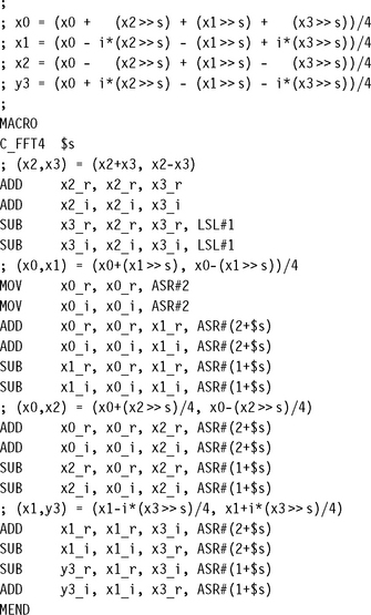
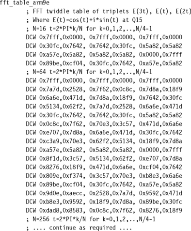
To implement the radix-4 butterfly efficiently, we use a radix-2 FFT to calculate DFT4. Provided that the input is bit-reversed, we can calculate a four-point DFT in place, in eight ARM registers. The following C_FFT4 macro lies at the heart of our FFT implementations. It performs the four-point DFT and input scale at the same time, which makes good use of the ARM barrel shifter. To prevent overflow, we also divide the answer by four.
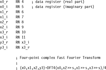
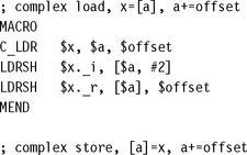
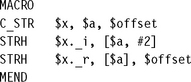
We will also use the following macros, C_LDR and C_STR, to load and store complex values. This will clarify the FFT code listing in Examples 8.17 and 8.18.
EXAMPLE 8.17
This example implements a 16-bit radix-4 FFT for any ARMv4 architecture processor. We assume that the number of points is n = 4b. If N is an odd power of two, then you will need to alter the routine to start with a radix-2 stage, or a radix-8 stage, rather than the radix-4 stage we show.
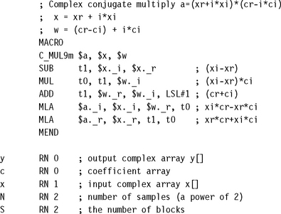
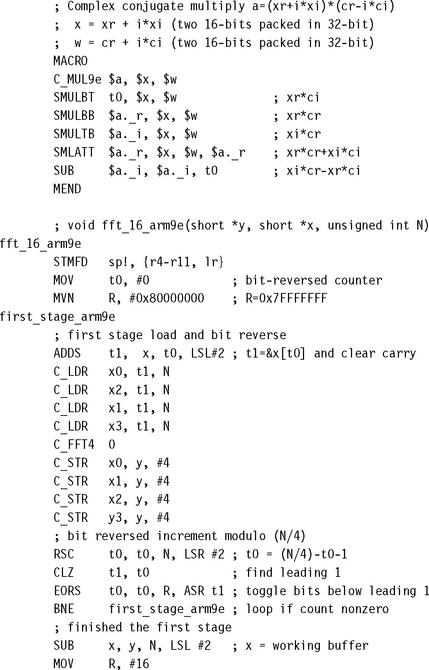
The code uses a trick to perform a complex multiply using only three real multiplies. If a + ib is a complex data item, and c + is a complex coefficient, then
When c + is = e2πi/N, these are the complex multiplies required for the forward and inverse transform radix-4 butterflies, respectively. Given inputs c – s, s, c + s, a, b, you can calculate either of the above using a subtract, multiply, and two multiply accumulates. In the coefficient lookup table we store (c – s, s) and calculate c + s on the fly. We can use the same table for both forward and inverse transforms.
Use the following code to perform the radix-4 transform on ARMv4. The number of points N must be a power of four. The algorithm actually calculates DFTN(x)/N, the extra scaling by N preventing overflow. The algorithm uses the C_FFT4 and load-store macros defined previously.
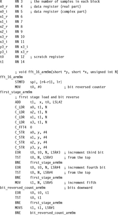
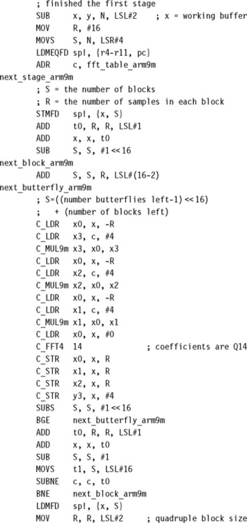
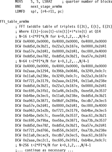
The code is in two parts. The first stage does not require any complex multiplies. We read the data in a bit-reversed order from the source array x, and then we apply the radix-4 butterfly and write to the destination array y. We perform the remaining stages in place in the destination buffer.
It is possible to implement the FFT without bit reversal, by alternating between the source and destination buffers at each stage. However, this requires more registers in the general stage loop, and there are none available. The bit-reversed increment is very cheap, costing less than 1.5 cycles per input sample in total.
See Section 8.6 for the benchmark results for the preceding code.
EXAMPLE 8.18
This example implements a radix-4 FFT on an ARMv5TE architecture processor such as the ARM9E. For the ARM9E we do not need to avail ourselves of the trick used in Example 8.17 to reduce a complex multiply to three real multiplies. With the single-cycle 16-bit × 16-bit multiplier it is faster to implement the complex multiply in the normal way. This also means that we can use a Q15 coefficient table of (c, s) values, and so the transform is slightly more accurate than in Example 8.17. We have omitted the register allocation because it is the same as for Example 8.17.
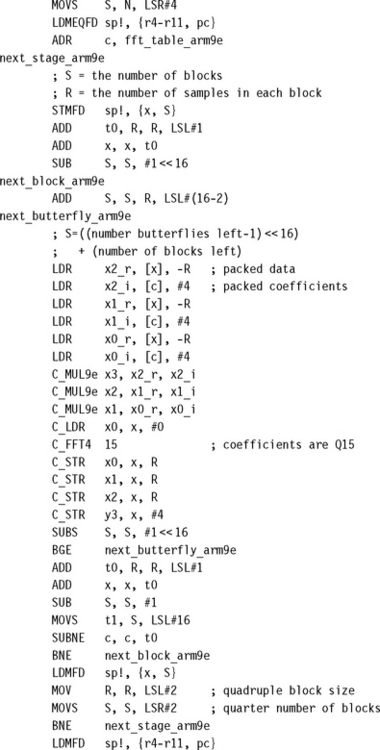
Once again, the routine actually calculates DFTN(x)/N, so that there is no possibility of overflow. Section 8.6 gives benchmark results for the preceding code.
Note that we use the CLZ instruction in ARMv5E to accelerate the bit-reversed count required for the bit reversal.
![]() Use a radix-4, decimation-in-time-based FFT implementation. If the number of points is not a power of four, then use radix-2 or radix-8 first stage.
Use a radix-4, decimation-in-time-based FFT implementation. If the number of points is not a power of four, then use radix-2 or radix-8 first stage.
![]() Perform bit reversal at the start of the algorithm, as you read data for the first stage. Although you can perform an FFT without bit reversal, this often requires more registers in the inner loop than are available.
Perform bit reversal at the start of the algorithm, as you read data for the first stage. Although you can perform an FFT without bit reversal, this often requires more registers in the inner loop than are available.
![]() If a scalar multiply requires more than one cycle, then reduce a complex multiply to three scalar multiplies using the trick of Example 8.17. This is the case for a 16-bit FFT on ARM9TDMI or a 32-bit FFT on ARM9E.
If a scalar multiply requires more than one cycle, then reduce a complex multiply to three scalar multiplies using the trick of Example 8.17. This is the case for a 16-bit FFT on ARM9TDMI or a 32-bit FFT on ARM9E.
![]() To prevent overflow, scale down by k in each radix-k stage. Alternatively ensure that the inputs to an N-point DFT have room to grow by N times. This is often the case when implementing a 32-bit FFT.
To prevent overflow, scale down by k in each radix-k stage. Alternatively ensure that the inputs to an N-point DFT have room to grow by N times. This is often the case when implementing a 32-bit FFT.
8.6 SUMMARY
Tables 8.9 and 8.10 summarize the performance obtained using the code examples of this chapter. It’s always possible to tune these routines further by unrolling, or coding for a specific application. However, these figures should give you a good idea of the sustained DSP performance obtainable in practice on an ARM system. The benchmarks include all load, store, and loop overheads assuming zero-wait-state memory or cache hits in the case of a cached core.
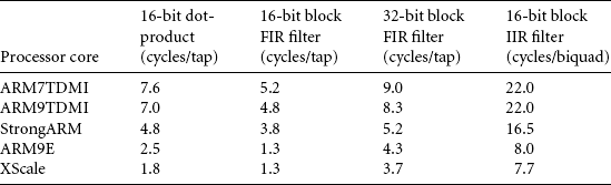
Table 8.10
| 16-bit complex FFT (radix-4) | ARM9TDMI (cycles/FFT) | ARM9E (cycles/FFT) |
| 64 point | 3,524 | 2,480 |
| 256 point | 19,514 | 13,194 |
| 1,024 point | 99,946 | 66,196 |
| 4,096 point | 487,632 | 318,878 |
In this chapter we have looked at efficient ways of implementing fixed-point DSP algorithms on the ARM. We’ve looked in detail at four common algorithms: dot-product, block FIR filter, block IIR filter, and Discrete Fourier Transform. We’ve also considered the differences between different ARM architectures and implementations.