
OPTIMIZED PRIMITIVES
7.1. DOUBLE-PRECISION INTEGER MULTIPLICATION
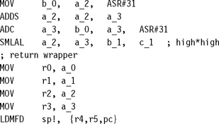
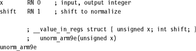
7.2. INTEGER NORMALIZATION AND COUNT LEADING ZEROS
7.3.1. Unsigned Division by Trial Subtraction
7.3.2. Unsigned Integer Newton-Raphson Division
7.5. TRANSCENDENTAL FUNCTIONS: LOG, EXP, SIN, COS
7.6. ENDIAN REVERSAL AND BIT OPERATIONS
A primitive is a basic operation that can be used in a wide variety of different algorithms and programs. For example, addition, multiplication, division, and random number generation are all primitives. Some primitives are supported directly by the ARM instruction set, including 32-bit addition and multiplication. However, many primitives are not supported directly by instructions, and we must write routines to implement them (for example, division and random number generation).
This chapter provides optimized reference implementations of common primitives. The first three sections look at multiplication and division. Section 7.1 looks at primitives to implement extended-precision multiplication. Section 7.2 looks at normalization, which is useful for the division algorithms in Section 7.3.
The next two sections look at more complicated mathematical operations. Section 7.4 covers square root. Section 7.5 looks at the transcendental functions log, exp, sin, and cos. Section 7.6 looks at operations involving bit manipulation, and Section 7.7 at operations involving saturation and rounding. Finally, Section 7.8 looks at random number generation.
You can use this chapter in two ways. First, it is useful as a straight reference. If you need a division routine, go to the index and find the routine, or find the section on division. You can copy the assembly from the book’s Web site. Second, this chapter provides the theory to explain why each implementation works, which is useful if you need to change or generalize the routine. For example, you may have different requirements about the precision or the format of the input and output operands. For this reason, the text necessarily contains many mathematical formulae and some tedious proofs. Please skip these as you see fit!
We have designed the code examples so that they are complete functions that you can lift directly from the Web site. They should assemble immediately using the toolkit supplied by ARM. For constancy we use the ARM toolkit ADS1.1 for all the examples of this chapter. See Section A.4 in Appendix for help on the assembler format. You could equally well use the GNU assembler gas. See Section A.5 for help on the gas assembler format.
You will also notice that we use the C keyword __value_in_regs. On the ARM compiler armcc this indicates that a function argument, or return value, should be passed in registers rather than by reference. In practical applications this is not an issue because you will inline the operations for efficiency.
We use the notation Qk throughout this chapter to denote a fixed-point representation with binary point between bits k – 1 and k. For example, 0.75 represented at Q15 is the integer value 0x6000. See Section 8.1 for more details of the Qk representation and fixed-point arithmetic. We say “d < 0. 5 at Q15” to mean that d represents the value d2−15 and that this is less than one half.
7.1 DOUBLE-PRECISION INTEGER MULTIPLICATION
You can multiply integers up to 32 bits wide using the UMULL and SMULL instructions. The following routines multiply 64-bit signed or unsigned integers, giving a 64-bit or 128-bit result. They can be extended, using the same ideas, to multiply any lengths of integer. Longer multiplication is useful for handling the long long C type, emulating double-precision fixed- or floating-point operations, and in the long arithmetic required by public-key cryptography.
We use a little-endian notation for multiword values. If a 128-bit integer is stored in four registers a3, a2, a1, a0, then these store bits [127:96], [95:64], [63:32], [31:0], respectively (see Figure 7.1).
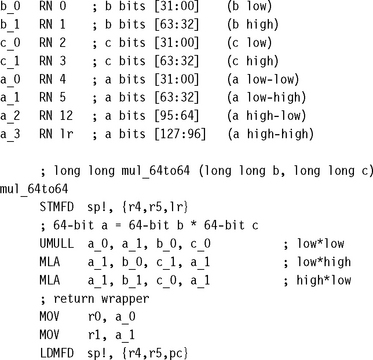
7.1.1 LONG LONG MULTIPLICATION
Use the following three-instruction sequence to multiply two 64-bit values (signed or unsigned) b and c to give a new 64-bit long long value a. Excluding the ARM Thumb Procedure Call Standard (ATPCS) wrapper and with worst-case inputs, this operation takes 24 cycles on ARM7TDMI and 25 cycles on ARM9TDMI. On ARM9E the operation takes 8 cycles. One of these cycles is a pipeline interlock between the first UMULL and MLA, which you could remove by interleaving with other code.
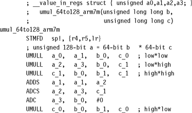
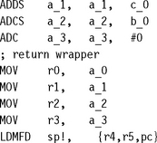
7.1.2 UNSIGNED 64-BIT BY 64-BIT MULTIPLY WITH 128-BIT RESULT
There are two slightly different implementations for an unsigned 64- by 64-bit multiply with 128-bit result. The first is faster on an ARM7M. Here multiply accumulate instructions take an extra cycle compared to the nonaccumulating version. The ARM7M version requires four long multiplies and six adds, a worst-case performance of 30 cycles.
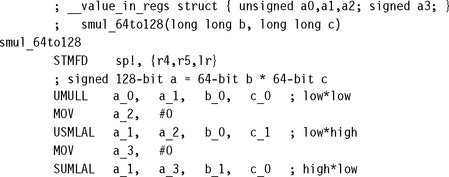
The second method works better on the ARM9TDMI and ARM9E. Here multiply accumulates are as fast as multiplies. We schedule the multiply instructions to avoid result-use interlocks on the ARM9E (see Section 6.2 for a description of pipelines and interlocks).
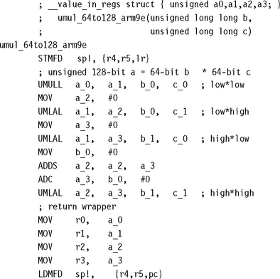
Excluding the function call and return wrapper, this implementation requires 33 cycles on ARM9TDMI and 17 cycles on ARM9E. The idea is that the operation ab + c + d cannot overflow an unsigned 64-bit integer if a, b, c, and d are unsigned 32-bit integers. Therefore you can achieve long multiplications with the normal schoolbook method of using the operation ab + c + d, where c and d are the horizontal and vertical carries.
7.1.3 SIGNED 64-BIT BY 64-BIT MULTIPLY WITH 128-BIT RESULT
A signed 64-bit integer breaks down into a signed high 32 bits and an unsigned low 32 bits. To multiply the high part of b by the low part of c requires a signed by unsigned multiply instruction. Although the ARM does not have such an instruction, we can synthesize one using macros.
The following macro USMLAL provides an unsigned-by-signed multiply accumulate operation. To multiply unsigned b by signed c, it first calculates the product bc considering both values as signed. If the top bit of b is set, then this signed multiply multiplied by the value b – 232. In this case it corrects the result by adding c232 . Similarly, SUMLAL performs a signed-by-unsigned multiply accumulate.
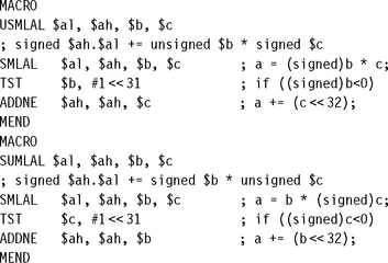
Using these macros it is relatively simple to convert the 64-bit multiply of Section 7.1.2 to a signed multiply. This signed version is four cycles longer than the corresponding unsigned version due to the signed-by-unsigned fix-up instructions.
7.2 INTEGER NORMALIZATION AND COUNT LEADING ZEROS
An integer is normalized when the leading one, or most significant bit, of the integer is at a known bit position. We will need normalization to implement Newton-Raphson division (see Section 7.3.2) or to convert to a floating-point format. Normalization is also useful for calculating logarithms (see Section 7.5.1) and priority decoders used by some dispatch routines. In these applications, we need to know both the normalized value and the shift required to reach this value.
This operation is so important that an instruction is available from ARM architecture ARMv5E onwards to accelerate normalization. The CLZ instruction counts the number of leading zeros before the first significant one. It returns 32 if there is no one bit at all. The CLZ value is the left shift you need to apply to normalize the integer so that the leading one is at bit position 31.
7.2.1 NORMALIZATION ON ARMv5 AND ABOVE
On an ARMv5 architecture, use the following code to perform unsigned and signed normalization, respectively. Unsigned normalization shifts left until the leading one is at bit 31. Signed normalization shifts left until there is one sign bit at bit 31 and the leading bit is at bit 30. Both functions return a structure in registers of two values, the normalized integer and the left shift to normalize.
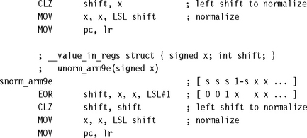
Note that we reduce the signed norm to an unsigned norm using a logical exclusive OR. If x is signed, then x^(x![]() 1) has the leading one in the position of the first sign bit in x.
1) has the leading one in the position of the first sign bit in x.
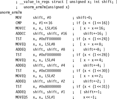
7.2.2 NORMALIZATION ON ARMv4
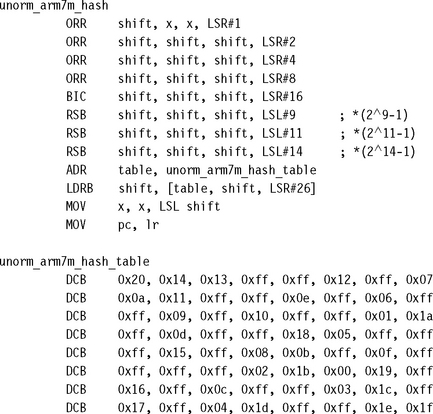
If you are using an ARMv4 architecture processor such as ARM7TDMI or ARM9TDMI, then there is no CLZ instruction available. Instead we can synthesize the same functionality. The simple divide-and-conquer method in unorm_arm7m gives a good trade-off between performance and code size. We successively test to see if we can shift x left by 16, 8, 4, 2, and 1 places in turn.
![]()
The final MOVEQ sets shift to 32 when x is zero and can often be omitted. The implementation requires 17 cycles on ARM7TDMI or ARM9TDMI and is sufficient for most purposes. However, it is not the fastest way to normalize on these processors. For maximum speed you can use a hash-based method.
The hash-based method first reduces the input operand to one of 33 different possibilities, without changing the CLZ value. We do this by iterating x = x | (x![]() s) for shifts s = 1, 2, 4, 8. This replicates the leading one 16 positions to the right. Then we calculate x = x &~(x
s) for shifts s = 1, 2, 4, 8. This replicates the leading one 16 positions to the right. Then we calculate x = x &~(x![]() 16). This clears the 16 bits to the right of the 16 replicated ones. Table 7.1 illustrates the combined effect of these operations. For each possible input binary pattern we show the 32-bit code produced by these operations. Note that the CLZ value of the input pattern is the same as the CLZ value of the code.
16). This clears the 16 bits to the right of the 16 replicated ones. Table 7.1 illustrates the combined effect of these operations. For each possible input binary pattern we show the 32-bit code produced by these operations. Note that the CLZ value of the input pattern is the same as the CLZ value of the code.
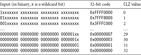
Now our aim is to get from the code value to the CLZ value using a hashing function followed by table lookup. See Section 6.8.2 for more details on hashing functions.
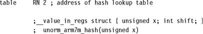
For the hashing function, we multiply by a large value and extract the top six bits of the result. Values of the form 2a + 1 and 2a – 1 are easy to multiply by on the ARM using the barrel shifter. In fact, multiplying by (29 – 1)(211 – 1)(214 – 1) gives a different hash value for each distinct CLZ value. The authors found this multiplier using a computer search.
You can use the code here to implement a fast hash-based normalization on ARMv4 processors. The implementation requires 13 cycles on an ARM7TDMI excluding setting up the table pointer.
7.2.3 COUNTING TRAILING ZEROS
Count trailing zeros is a related operation to count leading zeros. It counts the number of zeros below the least significant set bit in an integer. Equivalently, this detects the highest power of two that divides the integer. Therefore you can count trailing zeros to express an integer as a product of a power of two and an odd integer. If the integer is zero, then there is no lowest bit so the count trailing zeros returns 32.
There is a trick to finding the highest power of two dividing an integer n, for nonzero n. The trick is to see that the expression (n & (–n)) has a single bit set in position of the lowest bit set in n. Figure 7.2 shows how this works. The x represents wildcard bits.
Using this trick, we can convert a count trailing zeros to a count leading zeros. The following code implements count trailing zeros on an ARM9E. We handle the zero-input case without extra overhead by using conditional instructions.
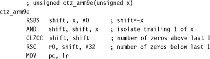
For processors without the CLZ instruction, a hashing method similar to that of Section 7.2.2 gives good performance:
7.3 DIVISION
ARM cores don’t have hardware support for division. To divide two numbers you must call a software routine that calculates the result using standard arithmetic operations. If you can’t avoid a division (see Section 5.10 for how to avoid divisions and fast division by a repeated denominator), then you need access to very optimized division routines. This section provides some of these useful optimized routines.
With aggressive optimization the Newton-Raphson division routines on an ARM9E run as fast as one bit per cycle hardware division implementations. Therefore ARM does not need the complexity of a hardware division implementation.
This section describes the fastest division implementations that we know of. The section is unavoidably long as there are many different division techniques and precisions to consider. We will also prove that the routines actually work for all possible inputs. This is essential since we can’t try all possible input arguments for a 32-bit by 32-bit division! If you are not interested in the theoretical details, skip the proof and just lift the code from the text.
Section 7.3.1 gives division implementations using trial subtraction, or binary search. Trial subtraction is useful when early termination is likely due to a small quotient, or on a processor core without a fast multiply instruction. Sections 7.3.2 and 7.3.3 give implementations using Newton-Raphson iteration to converge to the answer. Use Newton-Raphson iteration when the worst-case performance is important, or fast multiply instructions are available. The Newton-Raphson implementations use the ARMv5TE extensions. Finally Section 7.3.4 looks at signed rather than unsigned division.
We will need to distinguish between integer division and true mathematical division. Let’s fix the following notation:
![]() n/d = the integer part of the result rounding towards zero (as in C)
n/d = the integer part of the result rounding towards zero (as in C)
![]() n%d = the integer remainder n – d (n/d) (as in C)
n%d = the integer remainder n – d (n/d) (as in C)
![]() n//d = nd−1 =
n//d = nd−1 = ![]() = the true mathematical result of n divided by d
= the true mathematical result of n divided by d
7.3.1 UNSIGNED DIVISION BY TRIAL SUBTRACTION
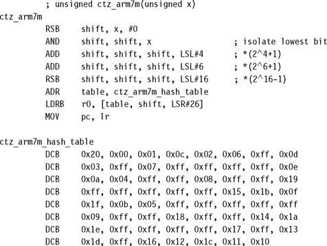
Suppose we need to calculate the quotient q = n/d and remainder r = n% d for unsigned integers n and d. Suppose also that we know the quotient q fits into N bits so that n/d < 2N, or equivalently n< (d ![]() N). The trial subtraction algorithm calculates the N bits of q by trying to set each bit in turn, starting at the most significant bit, bit N – 1. This is equivalent to a binary search for the result. We can set bit k if we can subtract (d
N). The trial subtraction algorithm calculates the N bits of q by trying to set each bit in turn, starting at the most significant bit, bit N – 1. This is equivalent to a binary search for the result. We can set bit k if we can subtract (d ![]() k) from the current remainder without giving a negative result. The example udiv_simple gives a simple C implementation of this algorithm:
k) from the current remainder without giving a negative result. The example udiv_simple gives a simple C implementation of this algorithm:
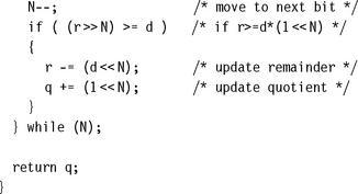
PROOF 7.1
To prove that the answer is correct, note that before we decrement N, the invariants of Equation (7.1) hold:
At the start q = 0 and r = n, so the invariants hold by our assumption that the quotient fits into N bits. Assume now that the invariants hold for some N. If r < d2N−1, then we need do nothing for the invariants to hold for N – 1. If r ≥ d2N−1, then we maintain the invariants by subtracting d2N–1 from r and adding 2N–1 to q.
The preceding implementation is called a restoring trial subtraction implementation. In a nonrestoring implementation, the subtraction always takes place. However, if r becomes negative, then we use an addition of (d ![]() N) on the next round, rather than a subtraction, to give the same result. Nonrestoring division is slower on the ARM so we won’t go into the details. The following subsections give you assembly implementations of the trial subtraction method for different numerator and denominator sizes. They run on any ARM processor.
N) on the next round, rather than a subtraction, to give the same result. Nonrestoring division is slower on the ARM so we won’t go into the details. The following subsections give you assembly implementations of the trial subtraction method for different numerator and denominator sizes. They run on any ARM processor.
7.3.1.1 Unsigned 32-Bit/32-Bit Divide by Trial Subtraction
This is the operation required by C compilers. It is called when the expression n/d or n%d occurs in C and d is not a power of 2. The routine returns a two-element structure consisting of the quotient and remainder.
To see how this routine works, first look at the code between the labels div_8bits and div_next. This calculates the 8-bit quotient r/d, leaving the remainder in r and inserting the 8 bits of the quotient into the lower bits of q. The code works by using a trial subtraction algorithm. It attempts to subtract 128d, 64d, 32d, 16d, 8d, 4d, 2d, and d in turn from r. For each subtract it sets carry to one if the subtract is possible and zero otherwise. This carry forms the next bit of the result to insert into q.
Next note that we can jump into this code at div_4bits or div_3bits if we only want to perform a 4-bit or 3-bit divide, respectively.
Now look at the beginning of the routine. We want to calculate r/d, leaving the remainder in r and writing the quotient to q. We first check to see if the quotient q will fit into 3 or 8 bits. If so, we can jump directly to div_3bits or div_8bits, respectively to calculate the answer. This early termination is useful in C where quotients are often small. If the quotient requires more than 8 bits, then we multiply d by 256 until r/d fits into 8 bits. We record how many times we have multiplied d by 256 using the high bits of q, setting 8 bits for each multiply. This means that after we have calculated the 8-bit r/d, we loop back to div_loop and divide d by 256 for each multiply we performed earlier. In this way we reduce the divide to a series of 8-bit divides.
7.3.1.2 Unsigned 32/15-Bit Divide by Trial Subtraction
In the 32/32 divide of Section 7.3.1.1, each trial subtraction takes three cycles per bit of quotient. However, if we restrict the denominator and quotient to 15 bits, we can do a trial subtraction in only two cycles per bit of quotient. You will find this operation useful for 16-bit DSP, where the division of two positive Q15 numbers requires a 30/15-bit integer division (see Section 8.1.5).
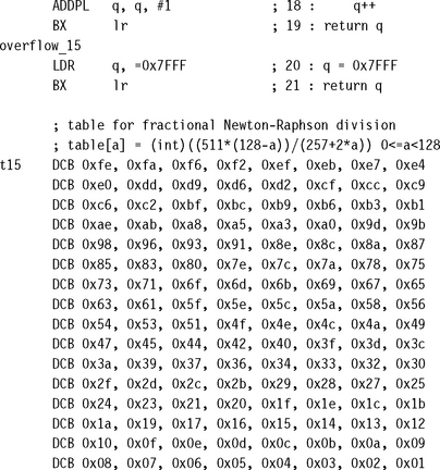
In the following code, the numerator n is a 32-bit unsigned integer. The denominator d is a 15-bit unsigned integer. The routine returns a structure containing the 15-bit quotient q and remainder r. If n ≥ (d ![]() 15), then the result overflows and we return the maximum possible quotient of 0x7fff.
15), then the result overflows and we return the maximum possible quotient of 0x7fff.
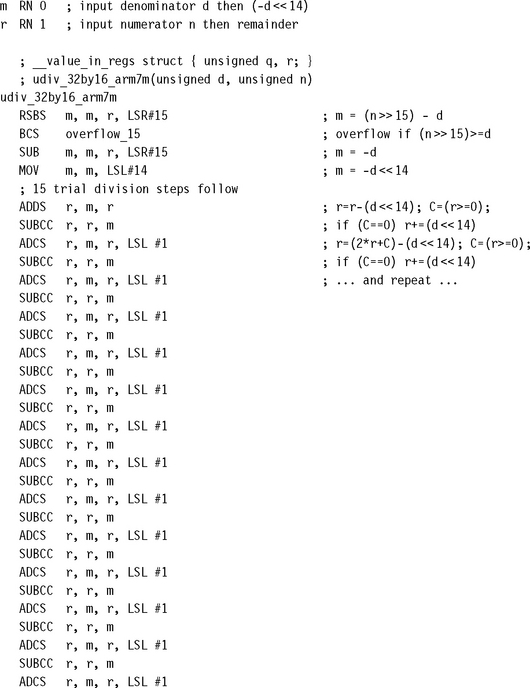
We start by setting m = –d214. Instead of subtracting a shifted version of the denominator from the remainder, we add the negated denominator to the shifted remainder. After the kth trial subtraction step, the bottom k bits of r hold the k top bits of the quotient. The upper 32 – k bits of r hold the remainder. Each ADC instruction performs three functions:
![]() It shifts the remainder left by one.
It shifts the remainder left by one.
![]() It inserts the next quotient bit from the last trial subtraction.
It inserts the next quotient bit from the last trial subtraction.
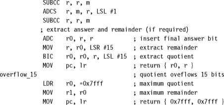
After 15 steps the bottom 15 bits of r contain the quotient and the top 17 bits contain the remainder. We separate these into r0 and r1, respectively. Excluding the return, the division takes 35 cycles on ARM7TDMI.
7.3.1.3 Unsigned 64/31-Bit Divide by Trial Subtraction
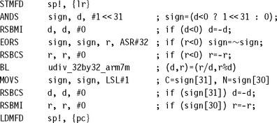
This operation is useful when you need to divide Q31 fixed-point integers (see Section 8.1.5). It doubles the precision of the division in Section 7.3.1.2. The numerator n is an unsigned 64-bit integer. The denominator d is an unsigned 31-bit integer. The following routine returns a structure containing the 32-bit quotient q and remainder r. The result overflows if n ≥ d232. In this case we return the maximum possible quotient of 0xffffffff. The routines takes 99 cycles on ARM7TDMI using a three-bit-per-cycle trial subtraction. In the code comments we use the notation [r, q] to mean a 64-bit value with upper 32 bits r and lower 32 bits q.
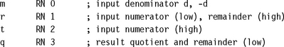
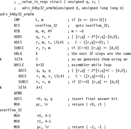
The idea is similar to the 32/15-bit division. After the kth trial subtraction the 64-bit value [r, q] contains the remainder in the top 64 – k bits. The bottom k bits contain the top k quotient bits. After 32 trial subtractions, r holds the remainder and q the quotient. The two ADC instructions shift [r, q] left by one, inserting the last answer bit in the bottom and subtracting the denominator from the upper 32 bits. If the subtraction overflows, we correct r by adding back the denominator.
7.3.2 UNSIGNED INTEGER NEWTON-RAPHSON DIVISION
Newton-Raphson iteration is a powerful technique for solving equations numerically. Once we have a good approximation of a solution to an equation, the iteration converges very rapidly on that solution. In fact, convergence is usually quadratic with the number of valid fractional bits roughly doubling with each iteration. Newton-Raphson is widely used for calculating high-precision reciprocals and square roots. We will use the Newton-Raphson method to implement 16- and 32-bit integer and fractional divides, although the ideas we will look at generalize to any size of division.
The Newton-Raphson technique applies to any equation of the form f(x) = 0, where f(x) is a differentiable function with derivative f’(x). We start with an approximation xn to a solution x of the equation. Then we apply the following iteration, to give us a better approximation xn+1
Figure 7.3 illustrates the Newton-Raphson iteration to solve f(x) = 0. 8 – x−1 = 0, taking x0 = 1 as our initial approximation. The first two steps are x1 = 1.2 and x2 = 1.248, converging rapidly to the solution 1.25.
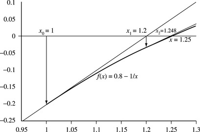
For many functions f, the iteration converges rapidly to the solution x. Graphically, we place the estimate xn+1 where the tangent to the curve at estimate xn meets the x-axis.
We will use Newton-Raphson iteration to calculate 2Nd−1 using only integer multiplication operations. We allow the factor of 2N because this is useful when trying to estimate 232/d as used in Sections 7.3.2.1 and 5.10.2. Consider the following function:
The equation f(x) = 0 has a solution at x = 2Nd−1 and derivative f’(x) = 2Nx−2. By substitution, the Newton-Raphson iteration is given by
In one sense the iteration has turned our division upside-down. Instead of multiplying by 2N and dividing by d, we are now multiplying by d and dividing by 2N. There are two cases that are particularly useful:
![]() N = 32 and d is an integer. In this case we can approximate 232d−1 quickly and use this approximation to calculate n/d, the ratio of two unsigned 32-bit numbers. See Section 7.3.2.1 for iterations using N = 32.
N = 32 and d is an integer. In this case we can approximate 232d−1 quickly and use this approximation to calculate n/d, the ratio of two unsigned 32-bit numbers. See Section 7.3.2.1 for iterations using N = 32.
![]() N = 0 and d is a fraction represented in fixed-point format with 0.5 ≤ d < 1. In this case we can calculate d−1 using the iteration, which is useful to calculate nd−1 for a range of fixed-point values n. See Section 7.3.3 for iterations using N = 0.
N = 0 and d is a fraction represented in fixed-point format with 0.5 ≤ d < 1. In this case we can calculate d−1 using the iteration, which is useful to calculate nd−1 for a range of fixed-point values n. See Section 7.3.3 for iterations using N = 0.
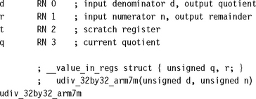
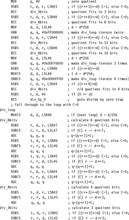
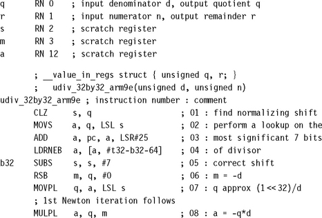
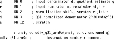
7.3.2.1 Unsigned 32/32-Bit Divide by Newton-Raphson
This section gives you an alterative to the routine of Section 7.3.1.1. The following routine has very good worst-case performance and makes use of the faster multiplier on ARM9E. We use Newton-Raphson iteration with N = 32 and integral d to approximate the integer 232/d. We then multiply this approximation by n and divide by 232 to get an estimate of the quotient q = n/d. Finally, we calculate the remainder r = n – qd and correct quotient and remainder for any rounding error.
PROOF 7.2
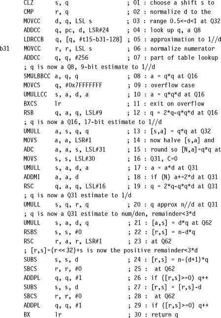
The proof that the code works is rather involved. To make the proof and explanation simpler, we comment each line with a line number for the instruction. Note that some of the instructions are conditional, and the comments only apply when the instruction is executed.
Execution follows several different paths through the code depending on the size of the denominator d. We treat these cases separately. We’ll use Ik as shorthand notation for the instruction numbered k in the preceding code.
Case 1 d = 0: 27 cycles on ARM9E, including return
We check for this case explicitly. We avoid the table lookup at I04 by making the load conditional on q ≠ 0. This ensures we don’t read off the start of the table. Since I01 sets s = 32, there is no branch at I09. I06 sets m = 0, and so I11 sets the Z flag and clears the carry flag. We branch at I15 to special case code.
Case 2 d = 1:27 cycles on ARM9E, including return
This case is similar to the d = 0 case. The table lookup at I05 does occur, but we ignore the result. I06 sets m = −1, and so I11 sets the Z and carry flags. The special code at I37 returns the trivial result of q = n, r = 0.
Case 3 2 ≤ d < 225: 36 cycles on ARM9E, including return
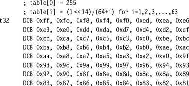
This is the hardest case. First we use a table lookup on the leading bits of d to generate an estimate for 232/d. I01 finds a shift s such that 231 ≤ d2s < 232. I02 sets a = d2s. I03 and I04 perform a table lookup on the top seven bits of a, which we will call i0. i0 is an index between 64 and 127. Truncating d to seven bits introduces an error f0:
We set a to the lookup value a0 = table[i0 – 64]= ![]() , where 0 ≤ g0 ≤ 1 is the table truncation error. Then,
, where 0 ≤ g0 ≤ 1 is the table truncation error. Then,
Noting that i0 + f0 = 2s–25d from Equation 7.5 and collecting the error terms into e0:
Since 64 ≤ i0 ≤ i0 + f0 < 128 by the choice of s it follows that –f02−6 ≤ e0 ≤ g02−7. As d < 225, we know s ≥ 7. I05 and I07 calculate the following value in register q:
This is a good initial approximation for 232d−1, and we now iterate Newton-Raphson twice to increase the accuracy of the approximation. I08 and I10 update the values of registers a and q to a1 and q1 according to Equation (7.9). I08 calculates a1 using m = –d. Since d ≥ 2, it follows that q0 < 231 for when d = 2, then f0 = 0, i0 = 64, g0 = 1, e0 = 2−8. Therefore we can use the signed multiply accumulate instruction SMLAWT at I10 to calculate q1.
The right shifts introduce truncation errors 0 ≤ f1 < 1 and 0 ≤ g1 < 1, respectively:
The new estimate q1 is more accurate with error e1 ≈ e02. I12, I13, and I14 implement the second Newton-Raphson iteration, updating registers a and q to the values a2 and q2:
Again the shift introduces a truncation error 0 ≤ g2 < 1:
Our estimate of 232d−1 is now sufficiently accurate. I16 estimates n/d by setting q to the value q3 in Equation (7.14). The shift introduces a rounding error 0 ≤ g3 < 1.
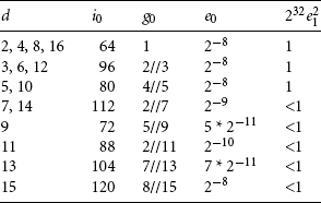
The error e3 is certainly positive and small, but how small? We will show that 0 ≤ e3 < 3, by showing that e21 < d2−32. We split into subcases:
Then f0 = f1 = g1 = 0 as the respective truncations do not drop any bits. So e1 = e02 and e0 = i0g02−14. We calculate i0 and g0 explicitly in Table 7.2.
Then f0 ≤ 0.5 implies |e0| ≤ 2−7. As f1 = g1 = 0, it follows that e12 ≤ 2−28 < d2−32.
Then f0 ≤ 1 implies |e0| ≤ 2−6. As f1 = g1 = 0, it follows that e12 ≤ 2−24 < d2−32.
Then f0 ≤ 1 implies |e0| ≤ 2−6. Therefore, e1 < 2−12 + 2−15 + d2−32. Let ![]() . Then 2−11.5 ≤ D < 2−3.5. So, e1 < D(2−0.5 + 2−3.5 + 2−3.5) < D, the required result.
. Then 2−11.5 ≤ D < 2−3.5. So, e1 < D(2−0.5 + 2−3.5 + 2−3.5) < D, the required result.
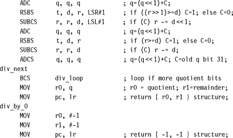
Now we know that e3 < 3, I16 to I23 calculate which of the three possible results q3, q3 + 1, q3 + 2, is the correct value for n/d. The instructions calculate the remainder r = n – dq3, and subtract d from the remainder, incrementing q, until 0 ≤ r < d.
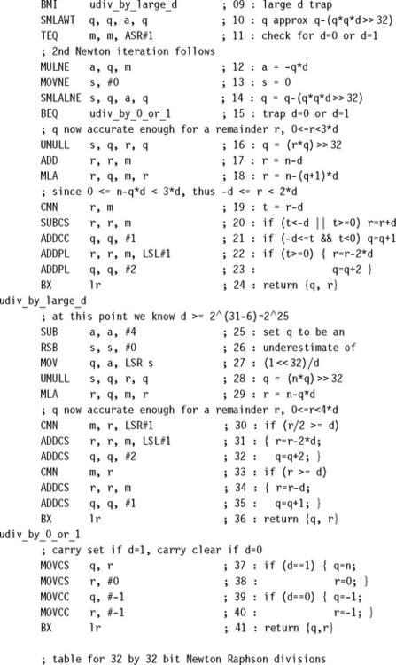
Case 4 225 ≤ d: 32 cycles on ARM9E including return
This case starts in the same way as Case 3. We have the same equation for i0 and a0. However, then we branch to I25, where we subtract four from a0 and apply a right shift of 7 – s. This gives the estimate q0 in Equation (7.15). The subtraction of four forces q0 to be an underestimate of 232d−1. For some truncation error 0 ≤ g0 < 1:
Since (232d−1)(![]() ) ≤ 2s+12−6 = 2s−5, it follows that 0 ≤ e0 < 3. I28 sets q to the approximated quotient g1. For some truncation error 0 < g1 < 1:
) ≤ 2s+12−6 = 2s−5, it follows that 0 ≤ e0 < 3. I28 sets q to the approximated quotient g1. For some truncation error 0 < g1 < 1:
Therefore q1 is an underestimate to n/d with error less than four. The final steps I28 to I35 use a two-step binary search to fix the exact answer. We have finished!
7.3.3 UNSIGNED FRACTIONAL NEWTON-RAPHSON DIVISION
This section looks at Newton-Raphson techniques you can use to divide fractional values. Fractional values are represented using fixed-point arithmetic and are useful for DSP applications.
For a fractional division, we first scale the denominator to the range 0.5 ≤ d < 1.0. Then we use a table lookup to provide an estimate x0 to d−1. Finally we perform Newton-Raphson iterations with N = 0. From Section 7.3.2, the iteration is
As i increases, xi becomes more accurate. For fastest implementation, we use low-precision multiplications when i is small, increasing the precision with each iteration.
The result is a short and fast routine. Section 7.3.3.3 gives a routine for 15-bit fractional division, and Section 7.3.3.4 a routine for 31-bit fractional division. Again, the hard part is to prove that we get the correct result for all possible inputs. For a 31-bit division we cannot test every combination of numerator and denominator. We must have a proof that the code works. Sections 7.3.3.1 and 7.3.3.2 cover the mathematical theory we require for the proofs in Sections 7.3.3.3 and 7.3.3.4. If you are not interested in this theory, then skip to Section 7.3.3.3.
Throughout the analysis, we stick to the following notation:
![]() d is a fractional value scaled so that 0. 5 ≤ d < 1.
d is a fractional value scaled so that 0. 5 ≤ d < 1.
![]() i is the stage number of the iteration.
i is the stage number of the iteration.
![]() ki is the number of bits of precision used for xi. We ensure that ki+1 > ki ≥ 3.
ki is the number of bits of precision used for xi. We ensure that ki+1 > ki ≥ 3.
With each iteration, we increase ki and reduce the error ei. First let’s see how to calculate a good initial estimate x0.
7.3.3.1 Theory: The Initial Estimate for Newton-Raphson Division
If you are not interested in Newton-Raphson theory, then skip the next two sections and jump to Section 7.3.3.3.
We use a lookup table on the most significant bits of d to determine the initial estimate x0 to d−1. For a good trade-off between table size and estimate accuracy, we index by the leading eight fractional bits of d, returning a nine-bit estimate x0. Since the leading bits of d and x0 are both one, we only need a lookup table consisting of 128 eight-bit entries.
Let a be the integer formed by the seven bits following the leading one of d. Then d is in the range (128 + a)2−8 ≤ d < (129 + a)2−8. Choosing c = (128.5 + a)2−8, the midpoint, we define the lookup table by
![]()
This is a floating-point formula, where round rounds to the nearest integer. We can reduce this to an integer formula that is easier to calculate if you don’t have floating-point support:
![]()
Clearly, all the table entries are in the range 0 to 255. To start the Newton-Raphson iteration we set x0 = 1 + table[a]2−8 and k0 = 9. Now we cheat slightly by looking ahead to Section 7.3.3.3. We will be interested in the value of the following error term:
First let’s look at d|e0|. If e0 ≤ 0, then
Running through the possible values of a, we find that d|e0| < 299 × 2−16. This is the best possible bound. Take d = (133 – e)2−16, and the smaller e > 0, the closer to the bound you will get! The same trick works for finding a sharp bound on E:
Running over the possible values of a gives us the sharp bound E < 2−15. Finally we need to check that x0 ≤ 2 – 2−7. This follows as the largest table entry is 254.
7.3.3.2 Theory: Accuracy of the Newton-Raphson Fraction Iteration
This section analyzes the error introduced by each fractional Newton-Raphson iteration:
It is often slow to calculate this iteration exactly. As xi is only accurate to at most ki of precision, there is not much point in performing the calculation to more than 2ki bits of precision. The following steps give a practical method of calculating the iteration. The iterations preserve the limits for xi and ei that we defined in Section 7.3.3.
2. Calculate an underestimate di to d, usually d to around 2ki bits. We only actually require that
3. Calculate, yi, a ki+1 + 1 bit estimate to dix2i in the range 0 ≤ yi < 4. Make yi as accurate as possible. However, we only require that the error gi satisfy
4. Calculate the new estimate xi+1 = 2xi – yi using an exact subtraction. We will prove that 0 ≤ xi +1 < 2 and so the result fits in ki+1 bits.
We must show that the new ki+1–bit estimate xi+1 satisfies the properties mentioned prior to Section 7.3.3.1 and calculate a formula for the new error ei+1. First, we check the range of xi+1:
The latter polynomial in xi has positive gradient for xi ≤ 2 and so reaches its maximum value when xi is maximum. Therefore, using our bound on gi,
On the other hand, since |ei| ≤ 0.5 and gi ≥ −0.25, it follows that
7.3.3.3 Q15 Fixed-Point Division by Newton-Raphson
We calculate a Q15 representation of the ratio nd−1, where n and d are 16-bit positive integers in the range 0 ≤ n < d < 215. In other words, we calculate
![]()
You can use the routine udiv_32by16_arm7m in Section 7.3.1.2 to do this by trial subtraction. However, the following routine calculates exactly the same result but uses fewer cycles on an ARMv5E core. If you only need an estimate of the result, then you can remove instructions I15 to I18, which correct the error of the initial estimate.
The routine veers perilously close to being inaccurate in many places, so it is followed by a proof that it is correct. The proof uses the theory of Section 7.3.3.2. The proof is a useful reference if the code requires adaptation or optimizing for another ARM core. The routine takes 24 cycles on an ARM9E including the return instruction. If d ≤ n < 215, then we return the saturated value 0x7fff.
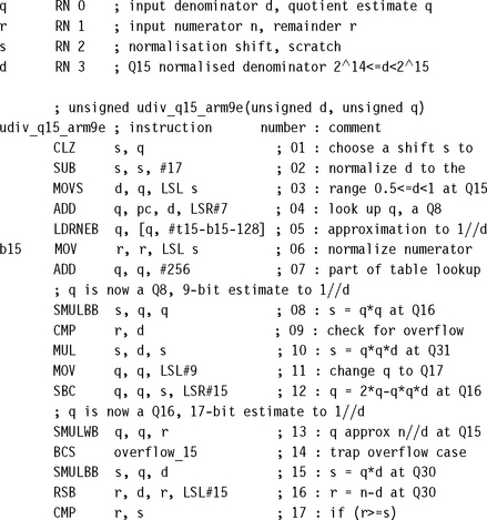
PROOF 7.3
The routine starts by normalizing d and n so that 214 ≤ d < 215 in instructions I01, I02, I03, I06. This doesn’t affect the result since we shift the numerator and denominator left by the same number of places. Considering d as a Q15 format fixed-point fraction, 0.5 ≤ d < 1. I09 and I14 are overflow traps that catch the case that n ≥ d. This includes the case d = 0. Assuming from now on that there is no overflow, I04, I05, I07 set q to the 9-bit Q8 initial estimate x0 to d−1 as described in Section 7.3.1.1. Since d is in the range 0. 5 ≤ d < 1, we subtract 128 on the table lookup so that 0.5 corresponds to the first entry of the table.
Next we perform one Newton-Raphson iteration. I08 sets a to the exact Q16 square of x0, and I10 sets a to the exact Q31 value of dx20. There is a subtlety here. We need to check that this value will not overflow an unsigned Q31 representation. In fact:
This term reaches its maximum value when x0 is as large as possible and e0 as negative as possible, which occurs when d = 0.5 + 2−8 – 2−15, where x0 = 2 – 2−7 and dx20 < 2 −−13 < 2 .
Finally I11 and I12 set q to a new Q16 estimate x1. Since the carry flag is clear from I09, the SBC underestimates the reciprocal.
Using Equation (7.33) for the new error:
I13 calculates a Q15 estimate q1 to the quotient nd−1:
where 0 ≤ h1 < 2−15 is the truncation error and
The bound on E is from Section 7.3.3.1. So, q1 is an underestimate to nd−1 of error less than 2−14. Finally I15, I16, I17, and I18 calculate the remainder n – qd and correct the estimate to Q15 precision.
7.3.3.4 Q31 Fixed-Point Division by Newton-Raphson
We calculate a Q31 representation of the ratio nd−1, where n and d are 32-bit positive integers in the range 0 ≤ n < d < 231. In other words we calculate
![]()
You can use the routine udiv_64by32_arm7m in Section 7.3.1.3 to do this by trial subtraction. However, the following routine calculates exactly the same result but uses fewer cycles on an ARM9E. If you only need an estimate of the result, then you can remove the nine instructions I21 to I29, which correct the error of the initial estimate.
As with the previous section, we show the assembly code followed by a proof of accuracy. The routine uses 46 cycles, including return, on an ARM9E. The routine uses the same lookup table as for the Q15 routine in Section 7.3.3.3.
PROOF 7.4
We first check that n < d. If not, then a sequence of conditional instructions occur that return the saturated value 0x7fffffff at I11. Otherwise d and n are normalized to Q31 representations, 230 ≤ d<231. I07 sets q to a Q8 representation of x0, the initial approximation, as in Section 7.3.3.3.
I08, I10, and I12 implement the first Newton-Raphson iteration. I08 sets a to the Q16 representation of x20. I10 sets a to the Q16 representation of dx20 − go, where the rounding error satisfies 0 ≤ g0 < 2−16. I12 sets x to the Q16 representation of x1, the new estimate to d−1. Equation (7.33) tells us that the error in this estimate is ![]() .
.
I13 to I19 implement the second Newton-Raphson iteration. I13 to I15 set a to the Q31 representation of ![]() for some error b1. As we use the ADC instruction at I15, the calculation rounds up and so 0 ≤ b1 ≤ 2−32. The ADC instruction cannot overflow since 233 – 1 and 234 – 1 are not squares. However, a1 can overflow a Q31 representation. I16 clears the carry flag and records in the N flag if the overflow takes place so that a1 ≥ 2. I17 and I18 set a to the Q31 representation of y1 = da1 – c1 for a rounding error 0 ≤ c1 < 2−31. As the carry flag is clear, I19 sets q to a Q31 representation of the new underestimate:
for some error b1. As we use the ADC instruction at I15, the calculation rounds up and so 0 ≤ b1 ≤ 2−32. The ADC instruction cannot overflow since 233 – 1 and 234 – 1 are not squares. However, a1 can overflow a Q31 representation. I16 clears the carry flag and records in the N flag if the overflow takes place so that a1 ≥ 2. I17 and I18 set a to the Q31 representation of y1 = da1 – c1 for a rounding error 0 ≤ c1 < 2−31. As the carry flag is clear, I19 sets q to a Q31 representation of the new underestimate:
I20 sets q to a Q31 representation of the quotient q2 = nx2 – b2 for some rounding error 0 ≤ b2 < 2−31. So:
If e1 ≥ 0, then d2e12 ≤ d4e02 < (2−15 – d2−16)2, using the bound on E of Section 7.3.3.1.
If e1 < 0, then d2e12 ≤ d2g02 < 2−32. Again, e3 < 3 × 2−31. In either case, q is an underestimate to the quotient of error less than 3 × 2−31. I21 to I23 calculate the remainder, and I24 to I29 perform two conditional subtracts to correct the Q31 result q.
7.3.4 SIGNED DIVISION
So far we have only looked at unsigned division implementations. If you need to divide signed values, then reduce them to unsigned divides and add the sign back into the result. The quotient is negative if and only if the numerator and denominator have opposite sign. The sign of the remainder is the sign of the numerator. The following example shows how to reduce a signed integer division to an unsigned division and how to calculate the sign of the quotient and remainder.
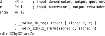
We use r12 to hold the signs of the quotient and remainder as udiv_32by32_arm7m preserves r12 (see Section 7.3.1.1).
7.4 SQUARE ROOTS
Square roots can be handled by the same techniques we used for division. You have a choice between trial subtraction and Newton-Raphson iteration based implementations. Use trial subtraction for a low-precision result less than 16 bits, but switch to Newton-Raphson for higher-precision results. Sections 7.4.1 and 7.4.2 cover trial subtraction and Newton-Raphson, respectively.
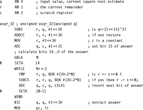
7.4.1 SQUARE ROOT BY TRIAL SUBTRACTION
We calculate the square root of a 32-bit unsigned integer d. The answer is a 16-bit unsigned integer q and a 17-bit unsigned remainder r such that
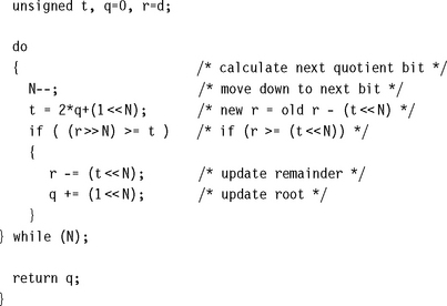
We start by setting q = 0 and r = d. Next we try and set each bit of q in turn, counting down from the highest possible bit, bit 15. We can set the bit if the new remainder is positive. Specifically if we set bit n by adding 2n to q, then the new remainder is
So, to calculate the new remainder we try to subtract the value 2n(2q + 2n). If the subtraction succeeds with a nonnegative result, then we set bit n of q. The following C code illustrates the algorithm, calculating the N-bit square root q of a 2N-bit input d:
![]()
Use the following optimized assembly to implement the preceding algorithm in only 50 cycles including the return. The trick is that register q holds the value (1 ![]() 30)|(q
30)|(q![]() (N + 1)) before calculating bit N of the answer. If we rotate this value left by 2N + 2 places, or equivalently right by 30 – 2N places, then we have the value t
(N + 1)) before calculating bit N of the answer. If we rotate this value left by 2N + 2 places, or equivalently right by 30 – 2N places, then we have the value t ![]() N, used earlier for the trial subtraction.
N, used earlier for the trial subtraction.
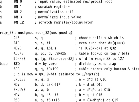
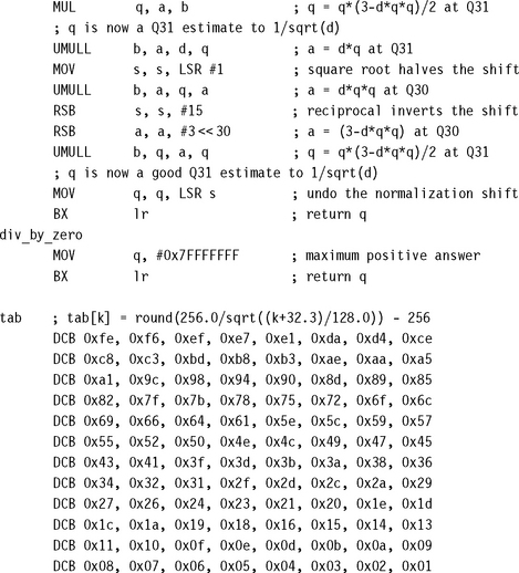
7.4.2 SQUARE ROOT BY NEWTON-RAPHSON ITERATION
The Newton-Raphson iteration for a square root actually calculates the value of d−0.5. You may find this is a more useful result than the square root itself. For example, to normalize a vector (x, y) you will multiply by
If you do require ![]() , then simply multiply d−0.5 by d. The equation f(x) = d – x−2 = 0 has positive solution x = d−0.5. The Newton-Raphson iteration to solve this equation is (see Section 7.3.2)
, then simply multiply d−0.5 by d. The equation f(x) = d – x−2 = 0 has positive solution x = d−0.5. The Newton-Raphson iteration to solve this equation is (see Section 7.3.2)
To implement this you can use the same methods we looked at in Section 7.3.2. First normalize d to the range 0. 25 ≤ d < 1. Then generate an initial estimate x0 using a table lookup on the leading digits of d. Iterate the above formula until you’ve achieved the precision required for your application. Each iteration will roughly double the number of significant answer bits.
The following code calculates a Q31 representation of the value d−0.5 for an input integer d. It uses a table lookup followed by two Newton-Raphson iterations and is accurate to a maximum error of 2−29. On an ARM9E the code takes 34 cycles including the return.
Similarly, to calculate ![]() you can use the Newton-Raphson iteration for the equation f(x) = d – x−k = 0.
you can use the Newton-Raphson iteration for the equation f(x) = d – x−k = 0.
7.5 TRANSCENDENTAL FUNCTIONS: LOG, EXP, SIN, COS
You can implement transcendental functions by using a combination of table lookup and series expansion. We examine how this works for the most common four transcendental operations: log, exp, sin, and cos. DSP applications use logarithm and exponentiation functions to convert between linear and logarithmic formats. The trigonometric functions sine and cosine are useful in 2D and 3D graphics and mapping calculations.
All the example routines of this section produce an answer accurate to 32 bits, which is excessive for many applications. You can accelerate performance by curtailing the series expansions with some loss in accuracy.
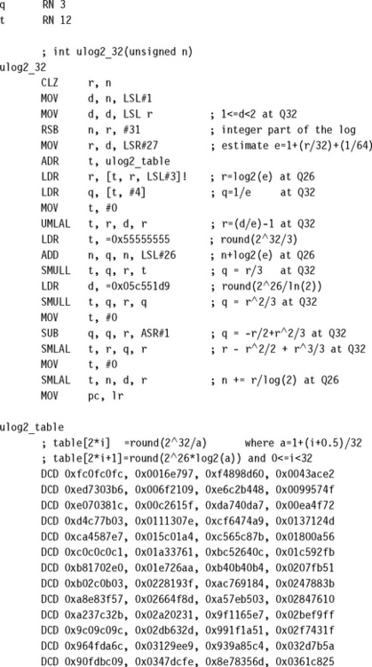
7.5.1 THE BASE-TWO LOGARITHM
Suppose we have a 32-bit integer n, and we want to find the base-two logarithm s = log2(n) suchthat n = 2s. Since s is in the range 0 ≤ s < 32, we will actually find a Q26 representation q of the logarithm so that q = s226. We can easily calculate the integer part of s using CLZ or the alternatives of Section 7.2. This reduces us to a number in the range 1 ≤ n < 2. First we perform a table lookup on an approximation a to n to find log2(a) and a−1. Since
we’ve reduced the problem to finding log2(na−1). As na−1 is close to one, we can use the series expansion of log2(1 + x) to improve the result accuracy:
where ln is the natural logarithm to base e. To summarize, we calculate the logarithm in three stages as illustrated in Figure 7.4:
![]() We use CLZ to find bits [31:26] of the result.
We use CLZ to find bits [31:26] of the result.
![]() We use a table lookup of the first five fractional bits to find an estimate.
We use a table lookup of the first five fractional bits to find an estimate.
![]() We use series expansion to calculate the estimate error more accurately.
We use series expansion to calculate the estimate error more accurately.
You can use the following code to implement this on an ARM9E processor using 31 cycles excluding the return. The answer is accurate to an error of 2−25.
![]()
![]()
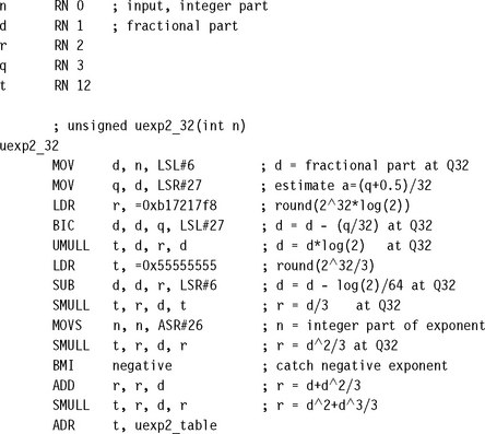
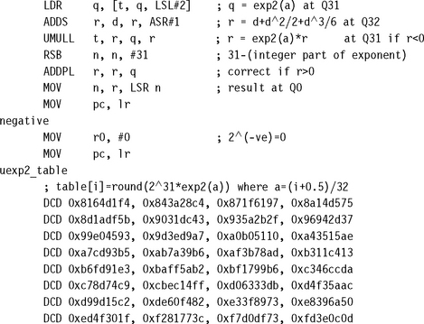
7.5.2 BASE-TWO EXPONENTIATION
This is the inverse of the operation of Section 7.5.1. Given a Q26 representation of 0 ≤ x < 32, we calculate the base-two exponent 2x. We start by splitting x into an integer part, n, and fractional part, d. Then 2x = 2d × 2n. To calculate 2d, first find an approximation a to d and look up 2a. Now,
Calculate x = (d – a)ln 2 and use the series expansion for exp(x) to improve the estimate:
You can use the following assembly code to implement the preceding algorithm. The answer has a maximum error of 4 in the result. The routine takes 31 cycles on an ARM9E excluding the return.
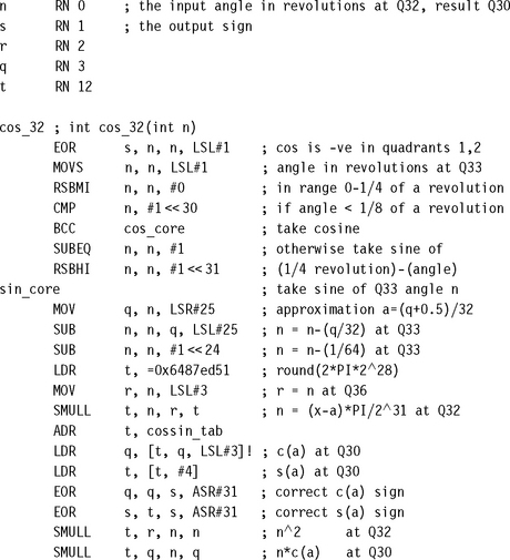
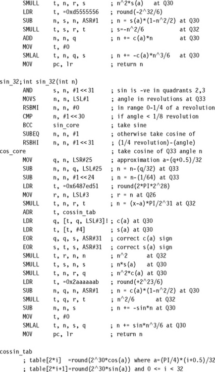
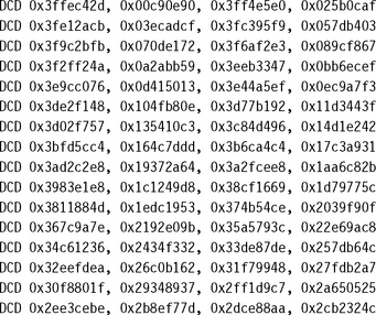
7.5.3 TRIGONOMETRIC OPERATIONS
If you need low-precision trigonometric operations (typically the case when generating sine waves and other audio signals, or for graphics processing), use a lookup table. For high-precision graphics or global positioning, greater precision may be required. The routines we look at here generate sine and cosine accurate to 32 bits.
The standard C library functions sin and cos specify the angle in radians. Radians are an awkward choice of units when dealing with optimized fixed-point functions. First, on any angle addition you need to perform arithmetic modulo 2π. Second, it requires range checking involving π to find out which quadrant of the circle an angle lies in. Rather than operate modulo 2π, we will operate modulo 232, a very easy operation on any processor.
Let’s define new base-two trigonometric functions s and c, where the angle is specified on a scale such that 232 is one revolution (2π radians or 360 degrees). To add these angles we use standard modular integer addition:
In this form, x is the Q32 representation of the proportion of a revolution represented by the angle. The top two bits of x tell us which quadrant of the circle the angle lies in. First we use the top three bits of x to reduce s(x) or c(x) to the sine or cosine of an angle between zero and one eighth of a revolution. Then we choose an approximation a to x and use a table to look up s(a) and c(a). The addition formula for sine and cosine reduces the problem to finding the sine and cosine of a small angle:
Next, we calculate the small angle n = π(x – a)2−31 in radians and use the following series expansions to improve accuracy further:
You can use the following assembly to implement the preceding algorithm for sine and cosine. The answer is returned at Q30 and has a maximum error of 4 × 2−30. The routine takes 31 cycles on an ARM9E excluding the return.
7.6 ENDIAN REVERSAL AND BIT OPERATIONS
This section presents optimized algorithms for manipulating the bits within a register. Section 7.6.1 looks at endian reversal, a useful operation when you are reading data from a big-endian file on a little-endian memory system. Section 7.6.2 looks at permuting bits within a word, for example, reversing the bits. We show how to support a wide variety of bit permutations. See also Section 6.7 for a discussion on packing and unpacking bitstreams.
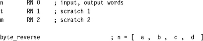
7.6.1 ENDIAN REVERSAL
To use the ARM core’s 32-bit data bus to maximum efficiency, you will want to load and store 8- and 16-bit arrays four bytes at a time. However, if you load multiple bytes at once, then the processor endianness affects the order they will appear in the register. If this does not match the order you want, then you will need to reverse the byte order.
You can use the following code sequences to reverse the order of the bytes within a word. The first sequence uses two temporary registers and takes three cycles per word reversed after a constant setup cycle. The second code sequence only uses one temporary register and is useful for reversing a single word.
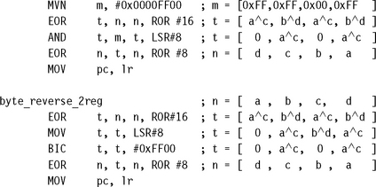
Halfword reversing within a word is provided free by the ARM barrel shifter since it is the same as a rotate right by 16 places.
7.6.2 BIT PERMUTATIONS
The byte reversal of Section 7.6.1 is a special case of a bit permutation. There are many other important bit permutations that you might come across (see Table 7.3):
Table 7.3
| Permutation name | Permutation action |
| Byte reversal | [b4, b3, b2, b1, b0] → [1 – b4, 1 – b3, b2, b1, b0] |
| Bit reversal | [b4, b3, b2, b1, b0] → [1 – b4, 1 – b3, 1 – b2, 1 – b1, 1 – b1] |
| Bit spread | [b4, b3, b2, b1, b0] → [b3, b2, b1, b0, b4] |
| DES permutation | [b5, b4, b3, b2, b1, b0] → [1 – b0, b2, b1, 1 – b5, 1 – b4, 1 – b3] |
![]() Bit reversal. Exchanging the value of bits k and 31 –k.
Bit reversal. Exchanging the value of bits k and 31 –k.
![]() Bit spreading. Spacing out the bits so that bit k moves to bit 2k for k < 16 and bit 2k – 31 for k ≥ 16.
Bit spreading. Spacing out the bits so that bit k moves to bit 2k for k < 16 and bit 2k – 31 for k ≥ 16.
![]() DES initial permutation. DES stands for the Data Encryption Standard, a common algorithm for bulk data encryption. The algorithm applies a 64-bit permutation to the data before and after the encryption rounds.
DES initial permutation. DES stands for the Data Encryption Standard, a common algorithm for bulk data encryption. The algorithm applies a 64-bit permutation to the data before and after the encryption rounds.
Writing optimized code to implement such permutations is simple when you have at hand a toolbox of bit permutation primitives like the ones we will develop in this section (see Table 7.4). They are much faster than a loop that examines each bit in turn, since they process 32 bits at a time.
Table 7.4
| Primitive name | Permutation action |
| A (bit index complement) | […,bk,…] → […,1 – bk,…] |
| B (bit index swap) | […,bj,…,bk,…] → […,bk,…,bj,…] |
| C (bit index complement+swap) | […,bj,…,bk,…] → […,1 – bk,…, 1 – bj,…] |
Let’s start with some notation. Suppose we are dealing with a 2k-bit value n and we want to permute the bits of n. Then we can refer to each bit position in n using a k-bit index ![]() . So, for permuting the bits within 32-bit values, we take k = 5. We will look at permutations that move the bit at position
. So, for permuting the bits within 32-bit values, we take k = 5. We will look at permutations that move the bit at position ![]() to position
to position ![]() , where each ci is either a bj or a1 – bj. We will denote this permutation by
, where each ci is either a bj or a1 – bj. We will denote this permutation by
For example, Table 7.3 shows the notation and action for the permutations we’ve talked about so far.
What’s the point of this? Well, we can achieve any of these permutations using a series of the three basic permutations in Table 7.4. In fact, we only need the first two since C is B followed by A twice. However, we can implement C directly for a faster result.
7.6.2.1 Bit Permutation Macros
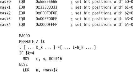
The following macros implement the three permutation primitives for a 32-bit word n. They need only four cycles per permutation if the constant values are already set up in registers. For larger or smaller width permutations, the same ideas apply.
7.6.2.2 Bit Permutation Examples
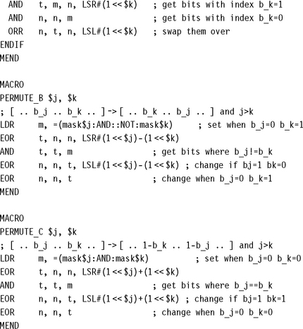
Now, let’s see how these macros will help us in practice. Bit reverse moves the bit at position b to position 31 – b; in other words, it inverts each bit of the five-bit position index b. We can use five type A transforms to implement bit reversal, logically inverting each bit index position in turn.
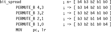
We can implement the more difficult bit spreading permutation using four type B transforms. This is only 16 cycles ignoring the constant setups—much faster than any loop testing each bit one at a time.
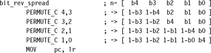
Finally, type C permutations allow us to perform bit reversal and bit spreading at the same time and with the same number of cycles.
7.6.3 BIT POPULATION COUNT
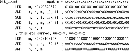
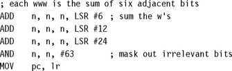
A bit population count finds the number of bits set within a word. For example, this is useful if you need to find the number of interrupts set in an interrupt mask. A loop testing each bit is slow, since ADD instructions can be used to sum bits in parallel provided that the sums do not interfere with each other. The idea of the divide by three and conquer method is to split the 32-bit word into bit triplets. The sum of each bit triplet is a 2-bit number in the range 0 to 3. We calculate these in parallel and then sum them in a logarithmic fashion.
Use the following code for bit population counts of a single word. The operation is 10 cycles plus 2 cycles for setup of constants.
7.7 SATURATED AND ROUNDED ARITHMETIC
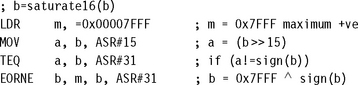
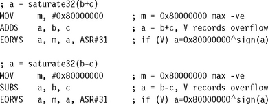
Saturation clips a result to a fixed range to prevent overflow. You are most likely to need 16- and 32-bit saturation, defined by the following operations:
![]() saturate16(x) = x clipped to the range −0x00008000 to +0x00007fff inclusive
saturate16(x) = x clipped to the range −0x00008000 to +0x00007fff inclusive
![]() saturate32(x) = x clipped to the range −0x80000000 to +0x7fffffff inclusive
saturate32(x) = x clipped to the range −0x80000000 to +0x7fffffff inclusive
We’ll concentrate on these operations although you can easily convert the 16-bit saturation examples to 8-bit saturation or any other length. The following sections give standard implementations of basic saturating and rounding operations you may need. They use a standard trick: for a 32-bit signed integer x,
x ![]() 31 = sign(x) = –1 if x < 0 and 0 if x ≥ 0
31 = sign(x) = –1 if x < 0 and 0 if x ≥ 0
7.7.1 SATURATING 32 BITS TO 16 BITS
This operation crops up frequently in DSP applications. For example, sound samples are often saturated to 16 bits before storing to memory. This operation takes three cycles, provided a constant m is set up beforehand in a register.
7.7.2 SATURATED LEFT SHIFT
In signal processing left shifts that could overflow need to saturate the result. This operation requires three cycles for a constant shift or five cycles for a variable shift c.
![]()
![]()
7.7.3 ROUNDED RIGHT SHIFT
A rounded shift right requires two cycles for a constant shift or three cycles for a nonzero variable shift. Note that a zero variable shift will only work properly if carry is clear.
![]()
7.8 RANDOM NUMBER GENERATION
To generate truly random numbers requires special hardware to act as a source of random noise. However, for many computer applications, such as games and modeling, speed of generation is more important than statistical purity. These applications usually use pseudorandom numbers.
Pseudorandom numbers aren’t actually random at all; a repeating sequence generates the numbers. However, the sequence is so long, and so scattered, that the numbers appear to be random. Typically we obtain Rk, the kth element of a pseudorandom sequence, by iterating a simple function of Rk−1:
For a fast pseudorandom number generator we need to pick a function f(x) that is easy to compute and gives random-looking output. The sequence must also be very long before it repeats. For a sequence of 32-bit numbers the longest length achievable is clearly 232.
A linear congruence generator uses a function of the following form.
![]()
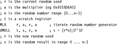
These functions are studied in detail in Knuth, Seminumerical Algorithms, Sections 3.2.1 and 3.6. For fast computation, we would like to take m = 232. The theory in Knuth assures us that if a % 8 = 5 and c = a, then the sequence generated has maximum length of 232 and is likely to appear random. For example, suppose that a = 0x91e6d6a5. Then the following iteration generates a pseudorandom sequence:
![]()
Since m is a power of two, the low-order bits of the sequence are not very random. Use the high-order bits to derive pseudorandom numbers of a smaller range. For example, set s = r ![]() 28 to generate a four-bit random number s in the range 0–15. More generally, the following code generates a pseudorandom number between 0 and n:
28 to generate a four-bit random number s in the range 0–15. More generally, the following code generates a pseudorandom number between 0 and n:
7.9 SUMMARY
ARM instructions only implement simple primitives such as addition, subtraction, and multiplication. To perform more complex operations such as division, square root, and trigonometric functions, you need to use software routines. There are many useful tricks and algorithms to improve the performance of these complex operations. This chapter covered the algorithms and code examples for a number of standard operations.
![]() using binary search or trial subtraction to calculate small quotients
using binary search or trial subtraction to calculate small quotients
![]() using Newton-Raphson iteration for fast calculation of reciprocals and extraction of roots
using Newton-Raphson iteration for fast calculation of reciprocals and extraction of roots
![]() using a combination of table lookup followed by series expansion to calculate transcendental functions such as exp, log, sin, and cos
using a combination of table lookup followed by series expansion to calculate transcendental functions such as exp, log, sin, and cos
![]() using logical operations with barrel shift to perform bit permutations, rather than testing bits individually
using logical operations with barrel shift to perform bit permutations, rather than testing bits individually
![]() using multiply accumulate instructions to generate pseudorandom numbers
using multiply accumulate instructions to generate pseudorandom numbers