Chapter 9. Business and Finance Problems
The need to solve business and finance problems is common to many Access users. While you can always export your data to Excel for analysis, it might be easier for you to find ways to solve these problems inside Access. Fortunately, using the capabilities found in the Access database engine and the VBA scripting language, you can tackle nearly any business or finance task.
In this chapter, you’ll learn how to solve a number of common problems, such as computing return on investment, straight-line depreciation, accelerated depreciation, interest, and moving averages. You’ll also learn how to use Access’ PivotTables and PivotCharts, which will help you decode some of the hidden information in your data.
Calculating Weighted Averages
Solution
You can use a SELECT statement like this to compute a weighted average:
	SELECT Sum(Value * Weight) / Sum(Weight) AS WeightedAverage
	FROM [Table9-1];
This statement will return the value in Figure 9-1 for the data found in Figure 9-2.
Discussion
To compute a weighted average, take the sum of the products of the values and the weights, and then divide the result by the sum of the weights. That is:
	                   Σ Vi * Wi
	Weighted Average = --------
	                     Σ Wi
where Vi represents the ith value and Wi represents the ith weight.


The key to understanding when to use weighted averages rather than simple averages is to look at how the items are related to each other. If all items have the same impact, you can use a simple average. But if the relative impacts of the items are different, you should use a weighted average.
For instance, when you are trying to compute the average price paid for a set of items, you should use a weighted average if the prices of the items vary. In this case, the price is the value, and the number of items is the weight. Computing the weighted average will give you an average price that is biased toward the price you paid for the most items.
Calculating a Moving Average
Solution
You can use a SELECT statement like the following to compute a moving average:
	SELECT A.Date, DisneyClose,
	  (Select Avg(DisneyClose)
	  From Stocks B
	  Where B.Date Between A.Date And DateAdd("d", -7, A.Date)) AS MovingAverage
	FROM Stocks AS A
	WHERE A.Date Between #1-1-2000# And #12-31-05#
	ORDER BY Date DESC;
This statement scans a table containing daily values, and uses a nested query to compute the average across the previous seven days.
You can easily adjust this range to change how the moving average is computed. For example, you could use a Where clause like this to compute the moving average over a 14-day window, with the current date in the middle:
Where B.Date Between DateAdd("d", 7, A.Date) And DateAdd("d", -7, A.Date)Discussion
A moving average is used to smooth time-series data that contains noticeable jumps between observations. The time scale for the observations can be days (as in the preceding example), months, or even years. Alternatively, you can use a simple AutoNumber column in place of a date field, since the values in that column will also increase over time.
The larger the range used to compute the moving average is, the smoother the resulting curve will be. In Figure 9-3, you can see how a moving average smoothes the individual observations of a stock price.
See Also

Calculating Payback Period
Solution
You can use the following routine to compute the payback period:
	Function PaybackPeriod(rs As ADODB.Recordset, Time As String, _
	    Interest As String, CashFlow As String, InitialInvestment As Currency) _
	    As Double

	Dim OldNPV As Currency
	Dim OldTime As Long
	Dim NPV As Currency
	Dim Temp As Currency

	NPV = 0
	OldTime = 0
	Do While Not rs.EOF
	   OldNPV = NPV
	   Temp = (1 + rs.Fields(Interest)) ^ rs.Fields(Time)
	   NPV = NPV + rs.Fields(CashFlow) / Temp
	   If NPV > InitialInvestment Then
	      PaybackPeriod = OldTime + _
	          (NPV - InitialInvestment) / (NPV - OldNPV) * (rs.Fields(Time) - OldTime)
	      Exit Function

	   End If

	   Debug.Print NPV, OldNPV, rs.Fields(Time), OldTime
	   OldTime = rs.Fields("Time")
	   rs.MoveNext

	Loop

	PaybackPeriod = -1

	End Function
To use this routine, you need to pass a Recordset object containing the information used to compute the net present value, along with the value of the initial investment. The result will be returned as a Double, representing the number of time periods needed to recover the initial investment. If the initial investment is not recovered within the series of data in the table, a value of -1 will be returned.
The following code shows how to call PaybackPeriod:
	Sub Example9_5()

	Dim rs As ADODB.Recordset
	Dim pp As Currency

	Set rs = New ADODB.Recordset
	Set rs.ActiveConnection = CurrentProject.Connection

	rs.Open "Select Time, InterestRate, CashFlow From [Table9-3]", , _
	   adOpenStatic, adLockReadOnly

	pp = PaybackPeriod(rs, "Time", "InterestRate", "CashFlow", 300)

	rs.Close

	Debug.Print "Payback period = ", pp

	End Sub
Discussion
Calculating the payback period is a way to determine the amount of time required to break even on an initial investment. Essentially, the PaybackPeriod routine computes the net present value for the supplied data on a time period-by-time period basis. When the current net present value exceeds the value of the initial investment, the initial investment is considered “paid back.”
Rather than simply returning the time period during which the investment was recovered, however, this routine also attempts to approximate the actual point at which it was recovered. Assuming a linear cash flow during each time period, the routine determines the percentage of the current time period’s cash flow that was needed to pay back the initial investment. This value is then multiplied by the difference in time between the current time period and the previous time period to give the approximate point during the current time period at which the investment was recovered.
Calculating Return on Investment
Problem
I need to know what the return on investment (ROI) will be for a particular set of cash flows.
Solution
This routine computes the ROI:
	Function ReturnOnInvestment(rs As ADODB.Recordset, Time As String, _
	    Interest As String, CashFlow As String, InitialInvestment As Currency) _
	    As Double

	Dim ROI As Currency
	Dim NPV As Currency

	NPV = NetPresentValue(rs, Time, Interest, CashFlow)

	ROI = (NPV - InitialInvestment) / InitialInvestment

	End Function

	Function NetPresentValue(rs As ADODB.Recordset, Time As String, _
	    Interest As String, CashFlow As String) As Currency

	Dim NPV As Currency
	Dim temp As Currency

	NPV = 0

	Do While Not rs.EOF
	   temp = (1 + rs.Fields(InterestRate)) ^ rs.Fields(Time)
	   NPV = NPV + rs.Fields(CashFlow) / temp

	   rs.MoveNext

	Loop

	rs.Close

	NetPresentValue = NPV

	End Function
The routine first calls the NetPresentValue function, using values returned in a recordset. It then computes the ROI by dividing the difference between the net present value and the initial investment by the initial investment.
Discussion
ROI gives you an indication of potential gain or loss on a particular investment. It is calculated using the following simple formula:
	                        Net Present Value − Initial Investment
	Return on Investment = -----------------------------------------
	                                   Initial Investment
Subtracting the initial investment from the net present value gives you the amount of money that the investment would yield; dividing this value by the initial investment gives you the percentage of change relative to the initial investment.
Calculating Straight-Line Depreciation
Solution
You can use the following function to compute straight-line depreciation:
	FunctionStraightLineDepreciation(Purchase As Currency, Salvage As Currency, _
	    UsefulLife As Long, Year As Long)

	StraightLineDepreciation = (Purchase - Salvage) / UsefulLife

	End Function
The StraightLineDepreciation function takes four parameters, but only three are used here. Purchase contains the initial purchase price of the item, while Salvage represents the salvage value of the item at the end of its useful life. UsefulLife contains the useful life of the item, in years. Year contains the year for which you wish to compute the depreciation; it’s ignored in this function, but was included to maintain the same set of parameters used in other depreciation functions.
The following routine shows how to use this function. It begins by opening an input table containing the items to be depreciated (see Figure 9-4). Then, it opens an empty table, which will hold the calculated depreciation for each year of each item’s useful life:

	Sub Example9_7()

	Dim intable As ADODB.Recordset
	Dim outtable As ADODB.Recordset

	Dim Year As Long
	Dim Purchase As Currency
	Dim Salvage As Currency
	Dim UsefulLife As Long

	Set intable = New ADODB.Recordset
	Set intable.ActiveConnection = CurrentProject.Connection
	intable.Open "Select Id, InitialPurchasePrice, SalvageValue, UsefulLife " & _
	    "From Inventory", , adOpenStatic, adLockReadOnly

	Set outtable = New ADODB.Recordset
	Set outtable.ActiveConnection = CurrentProject.Connection
	outtable.Open "[Table9-7]", , adOpenDynamic, adLockOptimistic

	Do While Not intable.EOF

	   Purchase = intable.Fields("InitialPurchasePrice")
	   Salvage = intable.Fields("SalvageValue")
	   UsefulLife = intable.Fields("UsefulLife")

	   For Year = 1 To UsefulLife
	      outtable.AddNew
	      outtable.Fields("Id") = intable.Fields("Id")
	      outtable.Fields("Year") = Year
	      outtable.Fields("StraightLine") =StraightLineDepreciation(Purchase, _
	          Salvage, UsefulLife, Year)
	      outtable.Update

	   Next Year

	   intable.MoveNext

	Loop

	intable.Close
	outtable.Close

	End Sub
For each item in the Inventory table, the data values used to compute depreciation are stored in a set of local variables. Then, a For loop is executed for each year of the item’s useful life. Inside the loop, a new row is added to the output table. This row contains Id, Year, and the newly computed depreciation value (see Figure 9-5). After all of the data has been processed, both tables are closed.

Discussion
Depreciation is a way to account for the fact that most items used in business lose value from the beginning of their lives until the end. Straight-line depreciation spreads the loss equally over each year of the item’s useful life:
	                             Initial Purchase Price − Salvage Value
	Straight-Line Depreciation = --------------------------------------
	                                          Useful Life
Of course, most items lose more of their value in earlier years than in later years. For example, consider a new car. Just driving it off the showroom floor decreases its value significantly, but the decrease in value between, say, years 10 and 11 is minimal. A more sophisticated version of this routine might attempt to calculate depreciation on a sliding scale. This is known as declining-balance depreciation.
Creating a Loan Payment Schedule
Problem
I would like to create a loan payment schedule that identifies the monthly payment amounts and the percentages of those amounts that are applied to interest and the principal, respectively.
Solution
You can use the following routine to calculate a loan payment schedule:
	Sub Example9_11()

	Dim intable As ADODB.Recordset
	Dim outtable As ADODB.Recordset

	Dim Year As Long
	Dim Principal As Currency
	Dim Interest As Double
	Dim LoanPeriod As Long
	Dim Payment As Currency
	Dim CurrentPrincipal As Currency
	Dim CurrentInterest As Double
	Dim i As Long

	Set intable = New ADODB.Recordset
	Set intable.ActiveConnection = CurrentProject.Connection
	intable.Open "Select Id, InitialPurchasePrice, LoanInterest, LoanPeriod " & _
	    "From Inventory", , adOpenStatic, adLockReadOnly

	Set outtable = New ADODB.Recordset
	Set outtable.ActiveConnection = CurrentProject.Connection
	outtable.Open "[Table9-11]", , adOpenDynamic, adLockOptimistic

	Do While Not intable.EOF

	   Principal = intable.Fields("InitialPurchasePrice")
	   Interest = intable.Fields("LoanInterest") / 12
	   LoanPeriod = intable.Fields("LoanPeriod")
	   Payment = LoanPayment(Principal, Interest, LoanPeriod)

	   For i = 1 To LoanPeriod
	      CurrentInterest = Principal * Interest
	      CurrentPrincipal = Payment - CurrentInterest
	      Principal = Principal - CurrentPrincipal

	      outtable.AddNew
	      outtable.Fields("Id") = intable.Fields("Id")
	      outtable.Fields("Period") = i
	      outtable.Fields("Payment") = Payment
	      outtable.Fields("Principal") = CurrentPrincipal
	      outtable.Fields("Interest") = CurrentInterest
	      outtable.Update

	   Next i

	   intable.MoveNext

	Loop

	intable.Close
	outtable.Close

	End Sub
This routine begins by defining two Recordset objects, intable and outtable. The intable Recordset reads an item from the Inventory table and extracts the information necessary to calculate the interest on a loan. The outtable Recordset maps to an empty table that will hold the loan payment schedules.
Next, the routine loops through the rows in the input table. Inside the loop it extracts the key fields into variables, taking care to ensure that the interest rate is converted from an annual rate to a monthly rate.
Once the variables are set, a For loop is used to process each month of the loan. The current principal and interest are calculated. Once the calculations are complete, the information for the month is written to the output table; once all of the months have been processed, the next row is read from intable.
Discussion
Storing the routine’s result in a table enables you to create reports to present the data. Figure 9-6 shows a simple report that lists key information about an item, including the repayment schedule for the loan taken out to purchase it.

Using PivotTables and PivotCharts
Solution
Access includes two data analysis tools that are similar to those found in Excel. A PivotTable (see Figure 9-7) is a way to summarize your data into a compact report while including the ability to expand particular sets of values to show the underlying detail. A PivotChart (see Figure 9-8) has the same basic features as a PivotTable, but the results are displayed graphically instead of as a tabular report.
Discussion
PivotTables and PivotCharts are ideal tools to use when you’re trying to understand your data, but don’t know where to begin. Because of their dynamic nature, you can quickly change the way the data is organized. This allows you to identify the information you want to present.


Excel also has PivotTables and PivotCharts, and Excel’s implementations are much more powerful than Access’. If you prefer, you can export your data to Excel and use Excel’s tools to analyze it. However, using PivotTables in Access has the advantage that you can quickly change the underlying query to retrieve different data and/or compute different values. One useful option is to use Access to tune your query and test your PivotTables and PivotCharts, and then export the data into Excel and use Excel’s capabilities to fine-tune the presentation of your data.
See Also
Creating PivotTables
Problem
How do I create a PivotTable?
Solution
You can create a PivotTable from a table or a query. First, open the table or query by double-clicking on its name. Then, in datasheet view, right-click on the window and choose PivotTable from the context menu. This will display an empty PivotTable similar to that shown in Figure 9-9.
There are four main areas in the PivotTable: the column area, the row area, the filter area, and the detail area. The column and row areas contain the fields whose values form the basic grid, while the filter area contains fields that can be used to include or exclude rows from the query.
The detail area occupies the bulk of the space in the PivotTable window, and represents the individual cells that make up the grid. In Figure 9-9, the detail section contains only the entry No Totals.
In addition to the PivotTable window itself, there are two other windows that you’ll use to create the table. The Field List window (the top-right window in Figure 9-9) contains the fields that you can use with your PivotTable. The Properties window (the lower-right window in Figure 9-9) contains properties of the PivotTable. These windows float above the other windows, and can easily be moved elsewhere on the screen, including outside the main Access window.
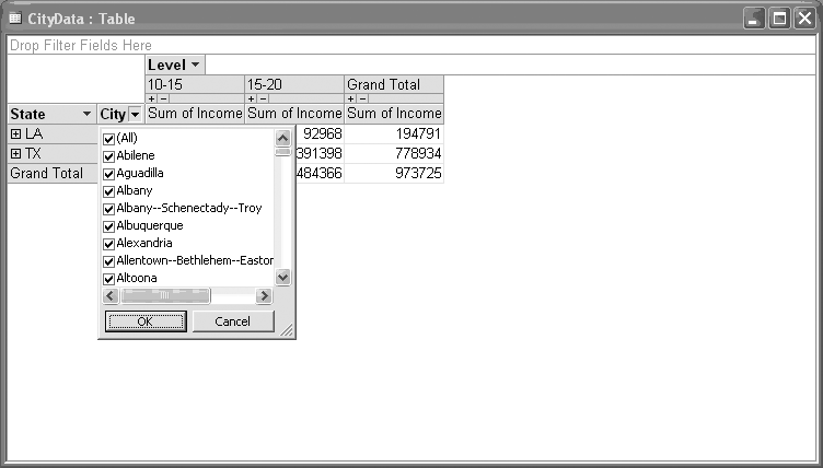
To populate your PivotTable, simply drag fields from the Field List window to the desired area in the PivotTable window. You can drag more than one field into each area. When you drag multiple fields into the row or column area, these fields are combined to form a nested index (see Figure 9-10).


The Grand Total column shown in Figure 9-10 represents the sum of the values displayed in each row. Hidden values are not included in this calculation, though there is an option you can choose that will perform calculations on all data, rather than just the visible data. You can choose which values are displayed by clicking on the arrows next to the field names and choosing values from the drop-down lists (see Figure 9-11).
Discussion
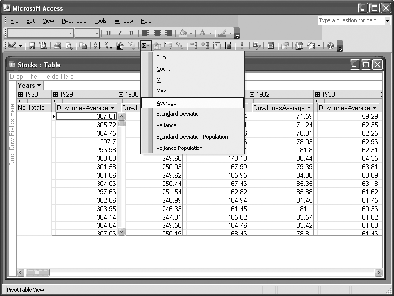
By default, Access computes the sum of the values you select. However, this isn’t appropriate in all circumstances. For example, if you were dealing with stock prices rather than populations, computing averages would be more appropriate. To see a list of the options that you can use to summarize the data in the PivotTable, either right-click on the value you wish to change and choose AutoCalc from the pop-up menu, or choose AutoCalc from the toolbar (see Figure 9-12).
If your data includes date values, Access will automatically generate a set of fields that you can use as columns or rows, which represent aggregations of date values. You can choose from three basic sets of fields: Date, Date By Week, and Date By Month (see Figure 9-13). These three fields also include automatically summarized fields that span years, quarters, months, weeks, days, hours, minutes, and seconds.
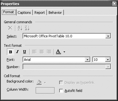
Setting properties in an Access PivotTable is a little different than it is in most applications. You can display the Properties window (shown in Figure 9-14) by right-clicking on the PivotTable window and choosing Properties from the context menu. While this appears to be a normal properties window, it behaves somewhat differently. Under “General commands” is a drop-down list. Choosing a different option from this list will display a different set of tabs, which contain properties specific to the selected item.
If you click on a field, you’ll be able to change the way the field is displayed in the PivotTable, along with its behavior. Clicking elsewhere on the PivotTable allows you to change the way information is displayed in the drag-and-drop areas (e.g., rows, columns, and filters), along with other general properties related to the PivotTable.

Charting Data
Problem
I want to analyze my data for trends, but looking at numbers is difficult for me. Is there a better alternative?
Solution
You can easily create a PivotChart using the result from any query. Simply run the query, right-click on the result, and choose PivotChart. Alternatively, you can work out which data you want to display in a PivotTable before switching the view to PivotChart (creating and working with PivotTables is covered in Creating PivotTables). Much of the structure will be carried over, including fields in the row, column, filter, and detail areas. If you’ve defined how the information is summarized in the PivotTable, those specifications will also be carried over. For example, the PivotTable shown in Figure 9-15 could be converted into the PivotChart shown in Figure 9-16 simply by right-clicking on the PivotTable and selecting PivotChart from the context menu.

Discussion
When dealing with PivotCharts, you need to consider the amount of data you want to display. As with any chart, it’s very easy to try to include too much data. Figure 9-17 shows what this can look like.
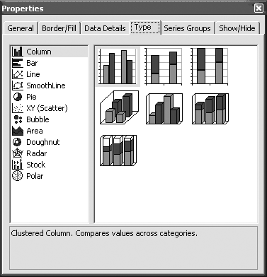
Of course, the amount of data you can comfortably include depends partly on the type of chart you’re displaying. Access supports most, but not all, of the chart types offered by Excel (see Figure 9-18). You can change the chart type by right-clicking a blank area in the chart and choosing Chart Type from the context menu.


As with a PivotTable, you can easily modify the way the data is displayed on a PivotChart. The interface for working with PivotCharts is the same as that for PivotTables; for more information, see Creating PivotTables.
Finding Trends
Problem
I have financial data that spans several months. At times, an upward or downward trend is apparent, but in some ranges of dates, the data is volatile and it’s hard to discern a trend.
What are some techniques to apply to large data sets to determine the overall trend?
Solution
The moving average (discussed in Calculating a Moving Average) is the de facto standard for pulling a trend out of seemingly random data. The approach used in Calculating a Moving Average computed an average based on calendar days, with all seven days of the week counted in the calculation. In this example, however, we’ll need to use actual data points without regard to the calendar.
Say you want to calculate 20- and 50-day moving averages for your data. Twenty data points are needed to get a 20-day moving average. But in financial markets, data is based on days the market is open (which excludes weekends and holidays). Thus, while the 20-day average will be based on 20 days of activity, the calendar spread will cover more than 20 days.
This routine calculates a 20- and 50-day moving average:
	Sub compute_moving_averages()
	Dim db As DAO.Database
	Dim rs As DAO.Recordset
	Dim ssql As String
	Dim sumit As Integer
	Dim avg20 As Single
	Dim avg50 As Single
	Set db = CurrentDb
	ssql = "Select * From Yahoo Order By Date"
	Set rs = db.OpenRecordset(ssql, dbOpenDynaset)
	'move down to the 20th row to start
	rs.Move 19
	Do While Not rs.EOF
	   avg20 = 0
	   rs.Move -19
	   For sumit = 1 To 20
	      avg20 = avg20 + rs.Fields("Close")
	      rs.MoveNext
	   Next sumit
	   If rs.EOF Then GoTo do_50
	   rs.Move -1 'put avg with correct ending date
	   rs.Edit
	   rs.Fields("20 day moving average") = avg20 / 20
	   rs.Update
	   rs.Move 1
	Loop
	do_50:
	rs.MoveFirst
	'move down to the 50th row to start
	rs.Move 49
	Do While Not rs.EOF
	   avg50 = 0
	   rs.Move -49
	   For sumit = 1 To 50
	      avg50 = avg50 + rs.Fields("Close")
	      rs.MoveNext
	   Next sumit
	   If rs.EOF Then GoTo endd
	   rs.Move -1 'put avg with correct ending date
	   rs.Edit
	   rs.Fields("50 day moving average") = avg50 / 50
	   rs.Update
	   rs.Move 1
	Loop
	endd:
	rs.Close
	Set rs = Nothing
	db.Close
	Set db = Nothing
	MsgBox "done"
	End Sub
In this case, the 20-day moving average starts on the 20th day in the data, and the 50-day moving average starts on the 50th day. Figure 9-19 shows the data points of the closing values for Yahoo! stock for July through December 2005. Between October and December, the data points are more erratic. The 20-day and 50-day moving averages provide a clearer picture of the stock’s direction.

There are other trend lines besides the moving average. Each follows a mathematical pattern, as illustrated in Table 9-1.
|
Type of trend line |
Formula |
|
Linear |
y = mx + b (m is the slope and b is the intercept) |
|
Logarithmic |
y = cln x + b |
|
Polynomial |
y = b + c1x + c2x2 + c3x3… |
|
Power |
y = cxb |
|
Exponential |
y = cebx |
In all the formulas in Table 9-1, y represents the positioning on the vertical (value) axis, and x represents the positioning on the horizontal (category) axis. While the formulas may look a bit complex if you are not math-savvy, an easy way to think of them is that y changes as x changes. On a chart, there is always a place where x and y intersect. Of course, other variables influence the value of y in each of these formulas.
Detailed explanations of the different types of trends are more in the realm of a good algebra or finance book, but let’s look briefly at a few examples. Figure 9-20 and Figure 9-21 show the Yahoo! data coupled with a linear trend line and a polynomial trend line, respectively. The trend lines appear different, but still clearly show the direction of the trend.


Discussion
Finding trends in data can help you intelligently guesstimate the direction the data may take within some future period (this is known as forecasting).
However, it’s important to consider that trends may be cyclical. Cyclical trends are trends that are expected to move in certain directions at different times, usually over the course of a year. This is a common phenomenon in some commodity markets. For example, the price of heating oil generally increases during cold months and decreases in warmer months. This is a standard case of prices being determined by supply and demand. More heating oil is needed in the winter than in the summer, and, all other things being equal, an increase in demand will raise prices, while a decrease in demand will lower prices.
A related but nearly opposite example is the cost of electricity. In summertime, the demand for electricity goes up (because all of the air conditioners are turned on); conversely, demand decreases in winter. Prices, to the extent of any market regulations, will go up along with the higher demand. Anyone care to guess the trend of air conditioner sales as the summer ends and autumn heads toward winter?
Finding Head and Shoulders Patterns
Problem
I’ve been studying the technical analysis of stocks, and I’ve read a lot about the so-called “Head and Shoulders” pattern. This is reasonably easy to identify when viewing a chart, but what’s a good routine that will look for the pattern just by testing data?
Solution
Head and Shoulders patterns found in sequential security prices serve as an investment tool to predict future price moves. The Head and Shoulders pattern does indeed resemble the general look of a head with a shoulder on each side. The pattern has these attributes:
A left shoulder, determined by ensuring that it is a pinnacle—that is, that the data point before and the data point after are both less than the shoulder data point.
A dip, or a point that is lower than the left shoulder, and is a nadir—that is, the data points before and after must be higher than the dip data point.
The head, which is a point higher than both shoulders. The head is a pinnacle.
A second dip, after the head, that is lower than the head and is a nadir.
The right shoulder, a pinnacle that comes after the second dip. This shoulder must be of a value that is between the head and the second dip.
That being said, there are variations on how to measure these data points. For example, must the second dip be lower than the first shoulder? Must the head be a certain percentage higher than the shoulders? Must all the data points lie within a given range of points? Clearly, identifying Head and Shoulders patterns involves a bit of art as well as financial acumen.
Figure 9-22 shows a chart in which the five key data points are enhanced with markers.

These points were identified via a code routine written in Access VBA. Working with a table of financial data containing the closing prices for Apple Computer stock, the shoulder, dip, and head points were determined with a couple of parameters used in the routine. In this case, a user enters the parameter values on an Access form. The first parameter is the range, which indicates how many sequential data points should be tested to see if a particular key data point (shoulder, dip, or head) has been found.
The second parameter is a percentage. This percentage is used in the routine as a guide for the minimum required difference between the vital data points. For example, the first dip must be at least the percentage amount lower than the first shoulder, the head must be at least the percentage amount above the first shoulder, and so on. Figure 9-23 shows the form and the results of running the procedure with the entered parameters. The listbox on the form displays the results of dates and data points that met the criteria. A complete set of points—shoulder1, dip1, head, dip2, shoulder2—is always returned. (By the way, the purported line running from dip1 to dip2 is called the "neckline.”)
Here is the code that locates the key values:
	Private Sub cmdFindPattern_Click()
	Dim head_flag As Boolean
	Dim shoulder1_flag As Boolean

	Dim shoulder2_flag As Boolean
	Dim dip1_flag As Boolean
	Dim dip2_flag As Boolean
	Dim head_date As Date
	Dim shoulder1_date As Date
	Dim shoulder2_date As Date
	Dim dip1_date As Date
	Dim dip2_date As Date
	Dim head_value As Single
	Dim shoulder1_value As Single
	Dim shoulder2_value As Single
	Dim dip1_value As Single
	Dim dip2_value As Single
	Dim rec_count As Integer
	Dim check_point As Single
	Dim last_close As Single
	Dim loop_1 As Integer
	Dim loop_2 As Integer
	Dim loop_3 As Integer
	Dim loop_4 As Integer
	Dim loop_5 As Integer
	Dim loop_6 As Integer
	Dim period_count As Integer
	Dim total_periods As Integer
	Dim percentage As Single
	Dim current_row As Integer
	Dim item_count As Integer

	'clear listbox
	For item_count = Me.listDataPoints.ListCount - 1 To 0 Step -1
	  Me.listDataPoints.RemoveItem (item_count)
	Next item_count

	'addheaders to listbox
	With Me.listDataPoints
	  .AddItem "Date;Close;Point Type", 0
	End With

	percentage = CSng(Me.txtPercent)

	Dim db As DAO.Database
	Set db = CurrentDb
	Dim rs As DAO.Recordset
	Set rs = db.OpenRecordset("Select * from Apple order by Date")
	rs.MoveLast
	rs.MoveFirst
	rec_count = rs.RecordCount
	period_count = 0
	total_periods = Me.txtPeriods
	head_flag = False
	shoulder1_flag = False
	shoulder2_flag = False
	dip1_flag = False
	dip2_flag = False
	'make sure that the number of units to analyze is not
	'bigger than the entire data set!
	If CInt(Me.txtPeriods) > rec_count Then
	   MsgBox "# of units bigger than recset"
	   Exit Sub
	End If

	On Error GoTo err_end
	start_row = 0
	current_row = 0
	For loop_1 = start_row To rec_count - 1
	  shoulder1_flag = False
	  shoulder1_date = Date
	  shoulder1_value = 0
	  dip1_flag = False
	  dip1_date = Date
	  dip1_value = 0
	  head_flag = False
	  head_date = Date
	  head_value = 0
	  dip2_flag = False
	  dip2_date = Date
	  dip2_value = 0
	  shoulder2_flag = False
	  shoulder2_date = Date
	  shoulder2_value = 0
	  total_datapoints = 0
	  period_count = 0
	  last_close = rs.Fields("Close")
	  rs.MoveNext
	  For loop_2 = current_row To rec_count - 1
	    If rs.Fields("Close") > (last_close * _
	          (1 + percentage)) Then
	       'shoulder must be a pinnacle - higher than the
	       'value before it and the value after it
	       rs.MovePrevious
	       check_point = rs.Fields("Close")
	       rs.MoveNext 'back to current position
	       If rs.Fields("Close") > check_point Then
	          rs.MoveNext
	          check_point = rs.Fields("Close")
	          rs.MovePrevious 'back to current position
	          If rs.Fields("Close") > check_point Then
	             shoulder1_flag = True
	             shoulder1_date = rs.Fields("Date")
	             shoulder1_value = rs.Fields("Close")
	             current_row = rs.AbsolutePosition
	             period_count = 0
	             Exit For
	          End If
	       End If
	    Else
	       period_count = period_count + 1
	       If period_count = total_periods Then Exit For
	       rs.MoveNext
	    End If
	  Next loop_2
	  Select Case shoulder1_flag
	    Case True
	      last_close = rs.Fields("Close")
	      rs.MoveNext
	      For loop_3 = current_row To rec_count - 1
	        If rs.Fields("Close") > shoulder1_value And shoulder1_flag = True Then
	           shoulder1_date = rs.Fields("Date")
	           shoulder1_value = rs.Fields("Close")
	        End If

	        If rs.Fields("Close") <= shoulder1_value * (1 - percentage) Then
	           'dip must be a nadir - lower than the value before it
	           'and the value after it
	           rs.MovePrevious
	           check_point = rs.Fields("Close")
	           rs.MoveNext 'back to current position
	           If rs.Fields("Close") < check_point Then
	              rs.MoveNext
	              check_point = rs.Fields("Close")
	              rs.MovePrevious 'back to current position
	              If rs.Fields("Close") < check_point Then
	                 dip1_flag = True
	                 dip1_date = rs.Fields("Date")
	                 dip1_value = rs.Fields("Close")
	                 current_row = rs.AbsolutePosition
	                 period_count = 0
	                 Exit For
	              End If
	           End If
	        Else
	           period_count = period_count + 1
	           If period_count = total_periods Then Exit For
	           rs.MoveNext
	        End If
	      Next loop_3
	      Select Case dip1_flag
	        Case True
	          last_close = rs.Fields("Close")
	          rs.MoveNext
	          For loop_4 = current_row To rec_count - 1
	            If rs.Fields("Close") < dip1_value And dip1_flag = True Then
	               dip1_date = rs.Fields("Date")
	               dip1_value = rs.Fields("Close")
	            End If
	            If (rs.Fields("Close") >= (shoulder1_value * (1 + percentage))) Then
	               'head must be a pinnacle - higher than the
	               'value before it and the value after it
	               rs.MovePrevious
	               check_point = rs.Fields("Close")
	               rs.MoveNext 'back to current position
	               If rs.Fields("Close") > check_point Then
	                  rs.MoveNext
	                  check_point = rs.Fields("Close")
	                  rs.MovePrevious 'back to current position
	                  If rs.Fields("Close") > check_point Then
	                     head_flag = True
	                     head_date = rs.Fields("Date")
	                     head_value = rs.Fields("Close")
	                     current_row = rs.AbsolutePosition
	                     period_count = 0
	                     Exit For
	                  End If
	               End If
	            Else
	               period_count = period_count + 1
	               If period_count = total_periods Then Exit For
	               rs.MoveNext
	            End If
	          Next loop_4
	          Select Case head_flag
	            Case True
	              last_close = rs.Fields("Close")
	              rs.MoveNext
	              For loop_5 = current_row To rec_count - 1
	                If rs.Fields("Close") > head_value And head_flag = True Then
	                   head_date = rs.Fields("Date")
	                   head_value = rs.Fields("Close")
	                End If
	                If rs.Fields("Close") < shoulder1_value Then
	                   'dip must be a nadir - lower than the value before it
	                   'and the value after it
	                   rs.MovePrevious
	                   check_point = rs.Fields("Close")
	                   rs.MoveNext 'back to current position
	                   If rs.Fields("Close") < check_point Then
	                      rs.MoveNext
	                      check_point = rs.Fields("Close")
	                      rs.MovePrevious 'back to current position
	                      If rs.Fields("Close") < check_point Then
	                         dip2_flag = True
	                         dip2_date = rs.Fields("Date")
	                         dip2_value = rs.Fields("Close")
	                         current_row = rs.AbsolutePosition
	                         period_count = 0
	                         Exit For
	                      End If
	                   End If
	                Else
	                   period_count = period_count + 1
	                   If period_count = total_periods Then Exit For
	                   rs.MoveNext
	                End If
	              Next loop_5
	              Select Case dip2_flag
	                Case True
	                  last_close = rs.Fields("Close")
	                  rs.MoveNext
	                  For loop_6 = current_row To rec_count - 1
	                    If rs.Fields("Close") < dip2_value And dip2_flag = True Then
	                       dip2_date = rs.Fields("Date")
	                       dip2_value = rs.Fields("Close")
	                    End If
	                    If (rs.Fields("Close") >= (dip2_value * _
	                          (1 + (percentage)))) And rs.Fields("Close") _
	                          < head_value Then
	                       'shoulder must be a pinnacle - higher than the
	                       'value before it and the value after it
	                       rs.MovePrevious
	                       check_point = rs.Fields("Close")
	                       rs.MoveNext 'back to current position
	                       If rs.Fields("Close") > check_point Then
	                          rs.MoveNext
	                          check_point = rs.Fields("Close")
	                          rs.MovePrevious 'back to current position
	                          If rs.Fields("Close") > check_point Then
	                             shoulder2_flag = True
	                             shoulder2_date = rs.Fields("Date")
	                             shoulder2_value = rs.Fields("Close")
	                             current_row = rs.AbsolutePosition
	                             period_count = 0
	                             Exit For
	                          End If
	                       End If
	                    Else
	                       rs.MoveNext
	                       period_count = period_count + 1
	                       If period_count = total_periods Then Exit For
	                    End If
	                  Next loop_6
	                  Select Case shoulder2_flag
	                    Case True
	                      'success!
	                      With Me.listDataPoints
	                        .AddItem "" & shoulder1_date & ";" & shoulder1_value & _
	                            ";Shoulder 1"
	                        .AddItem "" & dip1_date & ";" & dip1_value & ";Dip 1"
	                        .AddItem "" & head_date & ";" & head_value & ";Head"
	                        .AddItem "" & dip2_date & ";" & dip2_value & ";Dip 2"
	                        .AddItem "" & shoulder2_date & ";" & shoulder2_value & _
	                            ";Shoulder 2"
	                      End With
	                    Case False 'shoulder2_flag
	                  End Select 'shoulder2
	                Case False 'dip2
	              End Select 'dip2
	            Case False 'head
	          End Select 'head
	        Case False 'dip1
	      End Select 'dip1
	    Case False 'shoulder1
	  End Select 'shoulder1
	Next loop_1
	If Me.listDataPoints.ListCount = 0 Then
	   MsgBox "no patterns found"
	End If
	Exit Sub
	err_end:
	MsgBox "ran out of data - pattern not found"
	Err.Clear
	End Sub
This routine is a comprehensive shot at finding occurrences of the pattern in a data set. You might consider it as a springboard to a more intricate solution—for example, you might prefer to input a separate percentage for each leg of the pattern. Also, as it is, the routine uses the range input to control how many data points can exist between any two successive key data points. An additional input could control the overall range within which the five key data points must fall.
Discussion
Figure 9-22 showed the typical Head and Shoulders pattern generally used to find a reversal from an uptrend to a downtrend. This is also known as a “top” Head and Shoulders pattern.
The opposite and equally valid pattern is the “bottom” Head and Shoulders pattern, which resembles an upside-down head and shoulders. The dips are the two highest points, and the head is lower than the shoulders. This structure is used to find a reversal of a downtrend to an uptrend. Figure 9-24 shows what a bottom Head and Shoulders plot looks like.

The code to locate the key values in a bottom Head and Shoulders pattern is an alteration of the preceding routine. Only the portion of the routine that changes is shown here. The variables, Dim statements, and such are the same in both routines. Here is the rewritten section:
	For loop_2 = current_row To rec_count - 1
	  If (last_close - rs.Fields("Close")) / last_close > percentage Then
	     'shoulder must be a nadir - lower than the
	     'value before it and the value after it
	     rs.MovePrevious
	     check_point = rs.Fields("Close")
	     rs.MoveNext 'back to current position
	     If rs.Fields("Close") < check_point Then
	        rs.MoveNext
	        check_point = rs.Fields("Close")
	        rs.MovePrevious 'back to current position
	        If rs.Fields("Close") < check_point Then
	           shoulder1_flag = True
	           shoulder1_date = rs.Fields("Date")
	           shoulder1_value = rs.Fields("Close")
	           current_row = rs.AbsolutePosition
	           period_count = 0
	           Exit For
	        End If
	     End If
	  Else
	     period_count = period_count + 1
	     If period_count = total_periods Then Exit For
	     rs.MoveNext
	  End If
	Next loop_2
	Select Case shoulder1_flag
	  Case True
	    last_close = rs.Fields("Close")
	    rs.MoveNext
	    For loop_3 = current_row To rec_count - 1
	      If rs.Fields("Close") < shoulder1_valueAnd shoulder1_flag = True Then
	         shoulder1_date = rs.Fields("Date")
	         shoulder1_value = rs.Fields("Close")
	      End If
	      If rs.Fields("Close") > shoulder1_value * (1 + percentage) Then
	         'dip must be a pinnacle - higher than the value before it
	         'and the value after it
	         rs.MovePrevious
	         check_point = rs.Fields("Close")
	         rs.MoveNext 'back to current position
	         If rs.Fields("Close") > check_point Then
	            rs.MoveNext
	            check_point = rs.Fields("Close")
	            rs.MovePrevious 'back to current position
	            If rs.Fields("Close") > check_point Then
	               dip1_flag = True
	               dip1_date = rs.Fields("Date")
	               dip1_value = rs.Fields("Close")
	               current_row = rs.AbsolutePosition
	               period_count = 0
	               Exit For
	            End If
	         End If
	      Else
	         period_count = period_count + 1
	         If period_count = total_periods Then Exit For
	         rs.MoveNext
	      End If
	    Next loop_3
	    Select Case dip1_flag
	      Case True
	        last_close = rs.Fields("Close")
	        rs.MoveNext
	        For loop_4 = current_row To rec_count - 1
	          If rs.Fields("Close") > dip1_value And dip1_flag = True Then
	             dip1_date = rs.Fields("Date")
	             dip1_value = rs.Fields("Close")
	          End If
	          If (shoulder1_value - rs.Fields("Close")) / _
	                shoulder1_value > percentage Then
	             'head must be a nadir - lower than the value before it
	             'and the value after it
	             rs.MovePrevious
	             check_point = rs.Fields("Close")
	             rs.MoveNext 'back to current position
	             If rs.Fields("Close") < check_point Then
	                rs.MoveNext
	                check_point = rs.Fields("Close")
	                rs.MovePrevious 'back to current position
	                If rs.Fields("Close") < check_point Then
	                   head_flag = True
	                   head_date = rs.Fields("Date")
	                   head_value = rs.Fields("Close")
	                   current_row = rs.AbsolutePosition
	                   period_count = 0
	                   Exit For
	                End If
	             End If
	          Else
	             period_count = period_count + 1
	             If period_count = total_periods Then Exit For
	             rs.MoveNext
	          End If
	        Next loop_4
	        Select Case head_flag
	          Case True
	            last_close = rs.Fields("Close")
	            rs.MoveNext
	            For loop_5 = current_row To rec_count - 1
	              If rs.Fields("Close") < head_value And head_flag = True Then
	                 head_date = rs.Fields("Date")
	                 head_value = rs.Fields("Close")
	              End If
	              If rs.Fields("Close") > shoulder1_value * (1 + percentage) Then
	                 'dip must be a pinnacle - higher than the value before it
	                 'and the value after it
	                 rs.MovePrevious
	                 check_point = rs.Fields("Close")
	                 rs.MoveNext 'back to current position
	                 If rs.Fields("Close") > check_point Then
	                    rs.MoveNext
	                    check_point = rs.Fields("Close")
	                    rs.MovePrevious 'back to current position
	                    If rs.Fields("Close") > check_point Then
	                       dip2_flag = True
	                       dip2_date = rs.Fields("Date")
	                       dip2_value = rs.Fields("Close")
	                       current_row = rs.AbsolutePosition
	                       period_count = 0
	                       Exit For
	                    End If
	                 End If
	              Else
	                 period_count = period_count + 1
	                 If period_count = total_periods Then Exit For
	                 rs.MoveNext
	              End If
	            Next loop_5
	            Select Case dip2_flag
	              Case True
	                last_close = rs.Fields("Close")
	                rs.MoveNext
	                For loop_6 = current_row To rec_count - 1
	                  If rs.Fields("Close") > dip2_value And dip2_flag = True Then
	                     dip2_date = rs.Fields("Date")
	                     dip2_value = rs.Fields("Close")
	                  End If
	                  If (dip2_value - rs.Fields("Close")) / dip2_value > _
	                        percentage And rs.Fields("Close") > head_value Then
	                     'shoulder must be a nadir - lower than the
	                     'value before it and the value after it
	                     rs.MovePrevious
	                     check_point = rs.Fields("Close")
	                     rs.MoveNext 'back to current position
	                     If rs.Fields("Close") < check_point Then
	                        rs.MoveNext
	                        check_point = rs.Fields("Close")
	                        rs.MovePrevious 'back to current position
	                        If rs.Fields("Close") < check_point Then
	                           shoulder2_flag = True
	                           shoulder2_date = rs.Fields("Date")
	                           shoulder2_value = rs.Fields("Close")
	                           current_row = rs.AbsolutePosition
	                           period_count = 0
	                           Exit For
	                        End If
	                     End If
	                  Else
	                     rs.MoveNext
	                     period_count = period_count + 1
	                     If period_count = total_periods Then Exit For
	                  End If
	                Next loop_6
	                Select Case shoulder2_flag
	                  Case True
	                    'success!
	                    With Me.listDataPoints
	                      .AddItem "" & shoulder1_date & ";" & shoulder1_value & _
	                          ";Shoulder 1"
	                      .AddItem "" & dip1_date & ";" & dip1_value & ";Dip 1"
	                      .AddItem "" & head_date & ";" & head_value & ";Head"
	                      .AddItem "" & dip2_date & ";" & dip2_value & ";Dip 2"
	                      .AddItem "" & shoulder2_date & ";" & shoulder2_value & _
	                          ";Shoulder 2"
	                    End With
Working with Bollinger Bands
Solution
Bollinger Bands are a financial indicator that relates volatility with price over time. Given a set of sequential prices, to create Bollinger Bands, a moving average is created, and then the bands themselves are created on each side of the moving average. The bands are positioned two standard deviations away from each side of the moving average line. In other words, one band is created above the moving average line by adding the doubled standard deviation value to the moving average line. The other band sits under the moving average and is calculated by subtracting the doubled standard deviation from the moving average line.
Assuming you have a table filled with dates and prices, this query will return the moving average, the standard deviation, the doubled standard deviation value, the upper band, and the lower band. Price data from closing prices of McDonald’s stock is used in this statement. Substitute the table name with your table, and field names with yours, if required:
	SELECT A.Date, A.Close, (Select Avg(Close)
	From McDonalds B
	Where B.Date Between A.Date And DateAdd("d", -20, A.Date)) AS
	[20 Day Moving Average], (Select StDevP(Close)
	From McDonalds B
	Where B.Date Between A.Date And DateAdd("d", -20, A.Date)) AS
	[Standard Deviation], (Select StDevP(Close)  * 2
	From McDonalds B
	Where B.Date Between A.Date And DateAdd("d", -20, A.Date)) AS
	[2 Standard Deviations],
	[20 Day Moving Average]+[2 Standard Deviations] AS [Upper Band],
	[20 Day Moving Average]-[2 Standard Deviations] AS [Lower Band]
	FROM McDonalds AS A
	ORDER BY A.Date;
Figure 9-25 shows the result of running the query, and Figure 9-26 shows a plot of the data. Three series are in the chart: the moving average, the upper band, and the lower band. The standard deviation and doubled standard deviation values are included in the query for reference, but are not plotted.
Discussion
Bollinger Bands contract and expand around the moving average. This is an indicator of the volatility of the underlying price. Viewing the chart in Figure 9-26, it is apparent that the upper and lower bands are widest apart in the September–October period, and closer together in the rest of the plot. The wider the difference in the bands, the higher the volatility of the underlying data points. In fact, you could subtract the lower band from the upper band, over the time frame of the chart, to glean a clear picture of the deviation between the bands.


The chart shown in Figure 9-26 does not include the actual prices as a chart series,but you could include these in the chart. When price is included in the plot, it is the least smooth line, and it can actually cross the upper or lower band (providing buy or sell guidance).
For further information about Bollinger Bands, visit http://www.bollingerbands.com, or check out any comprehensive financial web site, such as Yahoo! Finance, or http://www.stockcharts.com.
Calculating Distance Between Zip Codes
Problem
I’ve seen several web sites where one can enter a zip code and a mileage amount, and then a list of stores, doctors, and other information within the defined region is returned. How is this done?
Solution
The trick is to use longitude and latitude settings. Each zip code is centered around a particular longitude and latitude intersection, and you’ll need a table containing these values. Lists are available on the Web. Some cost a bit, but others are free—run a search with “zip,” “longitude,” and “latitude” as keywords, and you’re bound to find many choices.
Figure 9-27 shows a section of a table that contains the necessary information.

Now, let’s consider the process. When a user enters a zip code on the web page, it has to be found in the zip code table to access its longitude and latitude values. A second scan of the zip table is then run to identify zip codes near the entered zip code. How near is “near” depends on the selected mileage setting. There is a formula to calculate what other zips are within the mileage parameter.
Longitude and latitude are measured in degrees, minutes, and seconds. Roughly, a degree is 69 miles, a minute is one-sixtieth of a degree (or 1.15 miles), and a second is about 100 feet.
These are approximations—nautical miles are measured differently than land miles, and there are other factors that affect longitude and latitude calculations.
A 1-mile variance of a longitude and latitude setting is a factor of approximately .008. A 10-mile variance is about .08.
This routine calculates a range around the entered zip code, in parameters of 10, 20, and 30 miles:
	Private Sub cmdFindZips_Click()
	Dim this_lat As Double
	Dim this_long As Double
	Dim conn As ADODB.Connection
	Dim rs As New ADODB.Recordset
	Dim drop_it As Integer
	'validation
	If Len(Me.txtZip) <> 5 Then
	   MsgBox "Enter a 5 digit zip code"
	   Exit Sub
	End If
	If IsNull(Me.lstMiles.Value) Then
	   MsgBox "Select a mileage range"
	   Exit Sub
	End If
	'setup
	For drop_it = Me.lstResults.ListCount - 1 To 0 Step -1
	   Me.lstResults.RemoveItem (drop_it)
	Next
	lblMatches.Caption = "Matches=0"
	'processing
	Set conn = CurrentProject.Connection
	ssql = "Select * from tblUSZipData Where Zip='" & Me.txtZip & "'"
	rs.Open ssql, conn, adOpenKeyset, adLockOptimistic
	If rs.RecordCount = 0 Then
	   rs.Close
	   Set rs = Nothing
	   Set conn = Nothing
	   MsgBox "Zip Not Found"
	   Exit Sub
	Else
	   this_lat = rs.Fields("Latitude")
	   this_long = rs.Fields("Longitude")
	   rs.Close
	   Select Case Me.lstMiles.Value
	     Case 10
	       ssql = "Select Zip, State, City from tblUSZipData Where " & _
	           "(Latitude Between " & this_lat + 0.08 & " and " _
	           & this_lat - 0.08 & ") And " & _
	           "(Longitude Between " & this_long + 0.05 & "and " _
	           & this_long - 0.05 & ")"
	     Case 20
	       ssql = "Select Zip, State, City from tblUSZipData Where " & _
	           "(Latitude Between " & this_lat + 0.17 & " and " _
	           & this_lat - 0.17 & ") And " & _
	           "(Longitude Between " & this_long + 0.17 & " and " _
	           & this_long - 0.17 & ")"
	     Case 30
	       ssql = "Select Zip, State, City from tblUSZipData Where " & _
	           "(Latitude Between " & this_lat + 0.26 & " and " _
	           & this_lat - 0.26 & ") And " & _
	           "(Longitude Between " & this_long + 0.26 & " and " _
	           & this_long - 0.26 & ")"
	   End Select
	   rs.Open ssql, conn, adOpenKeyset, adLockOptimistic
	   If rs.RecordCount = 0 Then
	      rs.Close
	      Set rs = Nothing
	      Set conn = Nothing
	      MsgBox "No Zips in Radius"
	      Exit Sub
	   Else
	      match = 0
	      Do Until rs.EOF
	         Me.lstResults.AddItem rs.Fields("Zip") & ";" & _
	             rs.Fields("City") & ";" & rs.Fields("State")
	         match = match + 1
	         rs.MoveNext
	      Loop
	      lblMatches.Caption = "Matches=" & match
	   End If 'If rs.RecordCount = 0 Then
	End If 'If rs.RecordCount = 0 Then
	rs.Close
	Set rs = Nothing
	Set conn = Nothing
	MsgBox "Done"
	End Sub
Figure 9-28 shows the entry form with a zip code entered and a mileage factor selected. The zip codes found within the designated range of the entered zip code are returned in a listbox.
Tip
The calculation in this routine looks for longitude and latitude settings that fit in a geographical box. Searching within a given radius requires a more complex calculation—check the Web for details. There is a lot more to know about how longitude and latitude work; with a little online research, you’ll be able to fine-tune your calculations to get more accurate results than those produced by the general solutions shown here.

Discussion
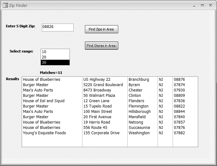
Finding zip codes in a certain area is useful if all you need are the zip codes. However, a more realistic application is to return a list of stores that are in the area surrounding the entered zip code.
The following code is a variation of the preceding routine. This time, a second table containing store names and addresses is involved. The tblCustomers table also contains the longitude and latitude for each store. In this variation, the tblCustomers table is queried, and the stores found within the area defined by the entered zip code and mileage range are returned in the listbox:
	Private Sub cmdFindStores_Click()
	Dim this_lat As Double
	Dim this_long As Double
	Dim conn As ADODB.Connection
	Dim rs As New ADODB.Recordset
	Dim drop_it As Integer
	'validation
	If Len(Me.txtZip) <> 5 Then
	   MsgBox "Enter a 5 digit zip code"
	   Exit Sub
	End If
	If IsNull(Me.lstMiles.Value) Then
	   MsgBox "Select a mileage range"
	   Exit Sub
	End If
	'setup
	For drop_it = Me.lstResults.ListCount - 1 To 0 Step -1
	   Me.lstResults.RemoveItem (drop_it)
	Next
	lblMatches.Caption = "Matches=0"
	'processing
	Set conn = CurrentProject.Connection
	ssql = "Select * fromtblUSZipData Where Zip='" & Me.txtZip & "'"
	rs.Open ssql, conn, adOpenKeyset, adLockOptimistic
	If rs.RecordCount = 0 Then
	   rs.Close
	   Set rs = Nothing
	   Set conn = Nothing
	   MsgBox "Zip Not Found"
	   Exit Sub
	Else
	   this_lat = rs.Fields("Latitude")
	   this_long = rs.Fields("Longitude")
	   rs.Close
	   Select Case Me.lstMiles.Value
	     Case 10
	       ssql = "Select Store, Address, City, State, Zip from tblCustomers " & _
	           "Where (Latitude Between " & this_lat + 0.08 & " and " _
	           & this_lat - 0.08 & ") And " & _
	           "(Longitude Between " & this_long + 0.05 & " and " _
	           & this_long - 0.05 & ")"
	     Case 20
	       ssql = "Select Store, Address, City, State, Zip from tblCustomers " & _
	           "Where (Latitude Between " & this_lat + 0.17 & " and " _
	           & this_lat - 0.17 & ") And " & _
	           "(Longitude Between " & this_long + 0.17 & " and " _
	           & this_long - 0.17 & ")"
	    Case 30
	      ssql = "Select Store, Address, City, State, Zip from tblCustomers " & _
	           "Where (Latitude Between " & this_lat + 0.26 & " and " _
	           & this_lat - 0.26 & ") And " & _
	           "(Longitude Between " & this_long + 0.26 & " and " _
	           & this_long - 0.26 & ")"
	   End Select
	   rs.Open ssql, conn, adOpenKeyset, adLockOptimistic
	   If rs.RecordCount = 0 Then
	      rs.Close
	      Set rs = Nothing
	      Set conn = Nothing
	      MsgBox "No Zips in Radius"
	      Exit Sub
	   Else
	      match = 0
	      Do Until rs.EOF
	         Me.lstResults.AddItem rs.Fields("Store") & ";" & _
	             rs.Fields("Address") & ";" & rs.Fields("City") & ";" & _
	             rs.Fields("State") & ";" & rs.Fields("Zip")
	         match = match + 1
	         rs.MoveNext
	      Loop
	      lblMatches.Caption = "Matches=" & match
	   End If 'If rs.RecordCount = 0 Then
	End If 'If rs.RecordCount = 0 Then
	rs.Close
	Set rs = Nothing
	Set conn = Nothing
	MsgBox "Done"
	End Sub
Figure 9-29 shows a returned list of stores found within the specified number of miles from the entered zip code.